The 2dF QSO Redshift Survey - XIII. A measurement of $\Lambda$ from the QSO power spectrum, $P^{S}(k_{\parallel},\mathbf{k}_{\perp})$

Abstract

We report on measurements of the cosmological constant, $\Lambda$, and the redshift space distortion parameter $\beta=\Omega_{m}^{0.6}/b$, based on an analysis of the QSO power spectrum parallel and perpendicular to the observer’s line of sight, $P^{S}(k_{\parallel},\mathbf{k}_{\perp})$, from the final catalogue of the 2dF QSO Redshift Survey. We derive a joint $\Lambda-\beta$ constraint from the geometric and redshift-space distortions in the power spectrum. By combining this result with a second constraint based on mass clustering evolution, we break this degeneracy and obtain strong constraints on both parameters. Assuming a flat ($\Omega_{\rm m}+\Omega_{\Lambda}=1$) cosmology and a $\Lambda$ cosmology $r(z)$ function to convert from redshift into comoving distance, we find best fit values of $\Omega_{\Lambda}=0.71^{+0.09}_{-0.17}$ and $\beta_{q}(z\sim 1.4)=0.45^{+0.09}_{-0.11}$. Assuming instead an EdS cosmology $r(z)$ we find that the best fit model obtained, with $\Omega_{\Lambda}=0.64^{+0.11}_{-0.16}$ and $\beta_{q}(z\sim 1.4)=0.40^{+0.09}_{-0.09}$, is consistent with the $\Lambda$ $r(z)$ results, and inconsistent with a $\Omega_{\Lambda}=0$ flat cosmology at over 95 per cent confidence.

1 Introduction

Observations of high redshift Type Ia Supernovae (SNIa) have recently generated much excitement and interest in $\Lambda$CDM cosmological models, deriving strong constraints on the cosmological constant, $\Lambda$ (e.g. Perlmutter et al. 1999; Riess et al. 1998). There are still uncertainties regarding the standard candle assumption that underlies this approach, however, and we don’t yet have a good understanding of SNIa physical processes. It is therefore important to develop independent ways to constrain $\Lambda$ in order to confirm this tantalizing result, as different methods suffer from different systematic uncertainties.

Different astronomical datasets are sensitive to different combinations of the cosmological parameters. For example, the recent WMAP cosmic microwave background (CMB) observations provide a strong constraint on $\Omega_{m}h^{2}$ (Spergel et al. 2003), whereas the shape of the matter power spectrum, probed by either galaxies (Percival et al. 2001) or QSOs (Outram et al. 2003), is sensitive to $\Omega_{m}h$. By combining several approaches we can break these degeneracies and hence derive much stronger constraints on the model that best describes our Universe (e.g. Efstathiou et al. 2002). Neither the CMB nor the large-scale structure observations, however, are directly sensitive to $\Omega_{\Lambda}$, and can only indirectly infer its value when the two datasets are combined.

Alcock & Paczyǹski (1979) suggested that $\Lambda$ might be measured directly from redshift-space distortions in the shape of large-scale structure, by making the simple assumption that clustering in real-space is on average spherically symmetric. Geometric distortions occur if the wrong cosmology is assumed, due to the different dependence on cosmology of the redshift-distance relation along and across the line of sight, and from the size of these geometric distortions, the true cosmology can be determined.

One approach to implementing this test is to use the distribution of QSOs to probe large-scale structure. By comparing the clustering of QSOs along and across the line of sight and modelling the effects of peculiar velocities and bulk motions in redshift space (Ballinger et al. 1996, Matsubara & Suto 1996), geometric distortions can be detected.

The ideal sample for this is the recently completed 2dF QSO Redshift Survey (2QZ). Data for 2QZ were obtained using the AAT 2dF facility. The completed survey comprises some 23000 $b_{\rm J}<20.85$ QSOs in two $5\times 75\deg^{2}$ declination strips, one at the South Galactic Pole and one in an equatorial region in the North Galactic Cap spanning the redshift range $0.3\la z\la 2.5$. The 2QZ catalogue and spectra were released in July 2003 (Croom et al. 2003) and can be obtained at http://www.2dfquasar.org.

Outram et al. (2001) produced a preliminary analysis of redshift-space distortions in the power spectrum, $P^{S}(k_{\parallel},\mathbf{k}_{\perp})$, of the incomplete 10k 2QZ survey (Croom et al. 2001). To help develop the method, and to test estimators designed to discriminate the effects of infall (measured via the parameter $\beta\sim\Omega_{m}^{0.6}/b$), small-scale velocity dispersion, and geometric distortions, a simulation of the 2QZ was used. Three light cone strips of the redshift survey were simulated, using the Virgo Consortium’s huge Hubble Volume N-body $\Lambda$CDM simulation (Frenk et al. 2000, Evrard et al. 2002). The effects of infall and geometry on the clustering distribution are very similar, and this approach alone could therefore only provide a degenerate constraint on $\Lambda$ and $\beta$. Outram et al. found, however, that this degeneracy could be broken by jointly considering a second constraint based on mass clustering evolution. Using the Hubble Volume simulation, Outram et al. predicted that this method should constrain $\beta$ to approximately $\pm 0.1$, and $\Omega_{\Lambda}$ to $\pm 0.25$ using the final 2QZ catalogue. A complementary approach, using the two-point correlation function, $\xi(\sigma,\pi)$, to investigate redshift-space distortions in QSO clustering can also be considered (Hoyle et al. 2002). Here we shall apply the analysis developed in Outram et al. to the final 2QZ sample, and hence derive this significant new constraint on $\Lambda$.

2 Power Spectrum Analysis

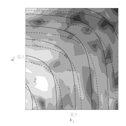
Figure 1: $P^{S}(k_{\parallel},\mathbf{k}_{\perp})$ determined from the 2QZ Catalogue assuming an EdS $r(z)$. Filled contours of constant ${\mathrm{l}og}(P(k)/h^{-3}$Mpc${}^{3})$ are shown as a function of $k_{\parallel}/h$ Mpc^-1 and ${\mathbf{k}}_{\perp}/h$ Mpc^-1. Overlaid are the best fit model (solid contours) with $\beta=0.40$ and $\Omega_{\Lambda}=0.64$, and for comparison, the best fitting flat $\Omega_{\Lambda}=0$ model with $\beta=0.27$ (dashed contours).

We reapply the analysis described in Outram et al. (2001) to the final 2QZ catalogue, containing 22652 QSOs (only those QSOs with quality 1 are used in this analysis; see Croom et al. (2003) for further details). For convenience we review the main details below.

2.1 The 2QZ selection function

We account for the various selection effects introduced into the 2QZ catalogue by generating a catalogue of random points that mimics the angular and radial selection functions of the QSOs but otherwise is unclustered. Details of the QSO selection function used can be found in Section 2.1 of Outram et al. (2003). We are measuring QSO clustering as a function of comoving distance, and so need to assume a cosmology in order to convert from redshift into comoving distance. Geometric distortions in the shape of large-scale structure occur if this cosmology is wrong, due to the different dependence on cosmology of the redshift-distance relation along and across the line of sight. From the size of these geometric distortions, measured in the QSO power spectrum, $P^{S}(k_{\parallel},\mathbf{k}_{\perp})$, the true cosmology can be determined. The choice of adopted cosmology shouldn’t matter in this analysis; adopting an incorrect cosmology does not affect the validity of this result. To check for consistency, however, we consider two possibilities; an Einstein-de Sitter ($\Omega_{\rm m}$=1.0, $\Omega_{\Lambda}$=0.0) cosmology $r(z)$ (EdS hereafter) and an $\Omega_{\rm m}$=0.3, $\Omega_{\Lambda}$=0.7 cosmology $r(z)$ ($\Lambda$ hereafter). To limit incompleteness, we restrict our analysis to $0.3<z<2.2$. This restricts our sample to 19549 QSOs with a mean redshift of $\bar{z}\sim 1.4$.

2.2 Power spectrum estimation

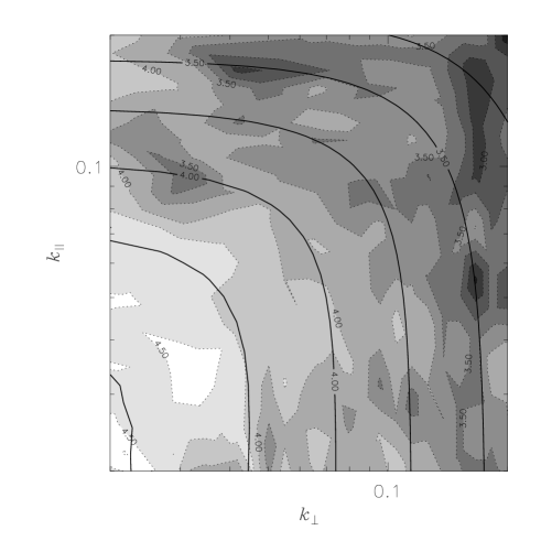
Figure 2: $P^{S}(k_{\parallel},\mathbf{k}_{\perp})$ determined from the 2QZ Catalogue assuming a $\Lambda$ $r(z)$. Filled contours of constant ${\mathrm{l}og}(P(k)/h^{-3}$Mpc${}^{3})$ are shown as a function of $k_{\parallel}/h$ Mpc^-1 and ${\mathbf{k}}_{\perp}/h$ Mpc^-1. Overlaid is the best fit model with $\beta=0.45$ and $\Omega_{\Lambda}=0.71$.

The power spectrum estimation is carried out as described in Outram, Hoyle & Shanks (2001). When calculating $P^{S}(k_{\parallel},\mathbf{k}_{\perp})$, information about the line of sight must be retained. To achieve this the data are divided into subsamples that subtend a small solid angle on the sky, and the distant-observer approximation is then applied. The data from each declination strip are split into 8 regions each approximately $5^{\circ}\times 10^{\circ}$ during this analysis. Each region is embedded into a larger cubical volume, which is rotated such that the central line of sight lies along the same axis of the cube in each case. The density field is binned onto a 256³ mesh, using nearest grid-point assignment. The power spectrum of each region is estimated using a Fast Fourier Transform (FFT), and the average of the resulting power spectra is taken. The results, binned logarithmically into $k_{\parallel}$ and $\mathbf{k}_{\perp}$, are plotted in Figure 1 (assuming an EdS $r(z)$) and Figure 2 (assuming a $\Lambda$ $r(z)$).

2.3 The window function

Figure 3: The power spectrum of the window function of the 2QZ catalogue, assuming $\Lambda$ $r(z)$, shown as a function of $k$. The solid squares show the points which were used in the analysis, with wavenumbers with $k_{\parallel}>0.02,|{\mathbf{k}}_{\perp}|>0.02$, and $k<0.2$. The dots show the power spectrum at smaller wavenumbers; excluded from this analysis. The window function is a steep power law, varying as $\sim k^{-3}$. For comparison, the open circles show the power spectrum of the window function from the analysis of the 2QZ 25k mock catalogue, and the crosses show the power spectrum of the window function from the analysis of the 2QZ 10k catalogue (Outram et al. 2001). The points are significantly lower than those of the 10k catalouge, due to the increased coverage, but still slightly higher than those of the mock catalogue due to the varying completeness pattern that still affects the finished survey (Croom et al. 2003). The overlaid line is a fit to the window function from the usual power spectrum analysis, binning in shells of $k$ (Outram et al. 2003).

The measured power spectrum is convolved with the power spectrum of the window function. The power spectrum of the window function is shown in figure 3. We compare the 2QZ window function to that of the 10k catalogue and the 25k mock catalogue determined in Outram et al. (2001). Due to the varying observational and spectroscopic incompleteness imprinted on the angular distribution of the 2QZ QSOs, the points lie slightly above those of the mock catalogue (where it was assumed that the angular distribution of the final catalogue would be uniform), but significantly lower than those of the 10k catalogue, due to the increased coverage. Outram et al. (2001; Section 2.3) adopted limits of $k_{\parallel}$ & $|\mathbf{k}_{\perp}|$ $\geq 0.02\;h\;$Mpc^-1 for the analysis of $P^{S}(k_{\parallel},\mathbf{k}_{\perp})$ to avoid any problems due to the effect of the window function on large scales. Whilst slightly higher than that of the mock catalogue, the window function is still sharply peaked in ${\mathbf{k}}$-space, and so we adopt the same limits in the case of the $\Lambda$ $r(z)$ analysis. Any window function effects should still be negligible. Assuming an EdS $r(z)$, however, the comoving distances probed are smaller, and hence the window function affects smaller scales. The appropriate limits to adopt in this case are $k_{\parallel}$ & $|\mathbf{k}_{\perp}|$ $\geq 0.03\;h\;$Mpc^-1.

2.4 Error estimates

A different error estimate is adopted in this paper from that of Outram et al. (2001). They adopted two methods to estimate the error in the power spectrum measurements; either via the dispersion between the power spectrum measurements from three declination strips of the Hubble Volume simulation, or the error estimate obtained using the method of Feldman, Kaiser & Peacock (FKP; 1994). The two estimates agree fairly well, but with large scatter. The FKP error is, on average, slightly lower than the error estimated from the dispersion betwen the three mock strips. Neither approach is ideal; the error estimated from the dispersion has a high uncertainty due to the small number of mock catalogues, and relies on the power of the mock catalogues being similar to that of the 2QZ catalogue, whereas the FKP error estimate assumes a thin shell geometry, and can under-estimate the error on some scales, due, for example, to the onset of non-linearity.

In order to apply the distant-observer approximation (see Section 2.2) the QSO power spectrum was estimated separately in sixteen individual $5^{\circ}\times 10^{\circ}$ regions. For this paper we have chosen to estimate the errors self-consistently from the data by considering the dispersion in these sixteen power spectrum measurements. As these regions are taken from just two contiguous strips, they lie next to each other, and are not entirely independent. It is therefore possible that they slightly underestimate the error in the power estimate, especially on large scales. Whilst we believe this effect would be small on the scales of interest, and hence do not consider it further in this paper, to test this fully would require several independent simulations of the survey, which are not currently available due to the large volume probed. This error estimate agrees well, on average, with estimates obtained from the Hubble Volume simulation (see section 2.4 of Outram et al. 2001), but is slightly larger than the FKP error estimate.

3 Modelling Redshift-space Distortions

The power spectrum model incorporating redshift distortions that we fit to the data is presented in Ballinger, Peacock and Heavens (1996), and briefly summarized below.

The power spectrum analysis was carried out assuming either an $\Omega_{\rm m}$=1.0, $\Omega_{\Lambda}$=0.0 cosmology or an $\Omega_{\rm m}$=0.3, $\Omega_{\Lambda}$=0.7 cosmology. If the true cosmology differs from this then geometric distortions will be introduced into the clustering pattern, due to the different dependence on cosmology of the redshift-distance relation along and across the line of sight. Our distance calculations will be wrong by a factor $f_{\perp}$ perpendicular to the line of sight, and $f_{\parallel}$ along the line of sight (as defined in Ballinger et al. 1996). Thus we can define a geometric flattening factor:

$$F(\Omega_{\Lambda},z)=\frac{f_{\parallel}}{f_{\perp}}$$ (1)

(Ballinger et al. 1996). The effect this has on the power spectrum is given by

$$P_{\mathrm{a}nisotropic}(k_{\parallel},{\mathbf{k}}_{\perp})=\frac{P_{\mathrm{t}rue}(k)}{f_{\perp}^{3+n}F}\left[1+\mu^{2}\left(\frac{1}{F^{2}}-1\right)\right]^{\frac{n}{2}}$$ (2)

(Ballinger et al. 1996) where $\mu=k_{\parallel}/k$, and $n$ is the spectral index of the power spectrum. By measuring the size of this geometric flattening, $F$, seen in the power spectrum $P^{S}(k_{\parallel},{\mathbf{k}}_{\perp})$, we can therefore calculate the true value of $\Omega_{\Lambda}$.

Unfortunately the problem is complicated by the fact that redshift-space distortions are also caused by peculiar velocities. The main cause of redshift-space distortions on the large linear scales probed by the QSO power spectrum are coherent peculiar velocities due to the infall of galaxies into overdense regions. This anisotropy takes a very simple form in redshift-space, depending only on the density and bias parameters via the combination $\beta\approx\Omega_{\rm m}^{0.6}/b$:

$$P^{S}(k_{\parallel},{\mathbf{k}}_{\perp})=P^{R}(k)\left[1+\beta\mu^{2}\right]^{2}$$ (3)

(Kaiser 1987) where $P^{S}$, and $P^{R}$ refer to the redshift-space and real-space power spectra respectively.

Whilst we expect the parameters $b$, $\Omega_{\rm m}$, and hence $\beta$ to vary as a function of redshift, we determine an average $P^{S}(k_{\parallel},{\mathbf{k}}_{\perp})$ over the redshift range $0.3<z<2.2$ from the 2QZ data, and hence only fit a single value of $\beta_{q}(z\sim 1.4)$ to the observed distortion. We consider the effect of allowing $\beta_{q}(z)$ to vary on the model, to test whether such variations could introduce systematic uncertainties, and whether the value of $\beta$ obtained represents a true average value for $\beta_{q}$ over the range $0.3<z<2.2$. Combining the redshift-space distortion power spectrum models generated using a varying $\beta_{q}(z)$, weighted using the QSO $n(z)$, we can determine an average model $P^{S}(k_{\parallel},{\mathbf{k}}_{\perp})$. We assume a simple bias model, designed to match the observations of Outram et al. (2003), where the QSO clustering amplitude increases linearly with redshift by 30 per cent from $z=0.3$ to $z=2.2$ (assuming $\Lambda$). In this evolving bias model, the best-fitting value of $\beta_{q}(z)$ increases with redshift from $\beta_{q}(0.3)=0.45$, reaching a maximum of $\beta_{q}(0.75)=0.51$, before decreasing to $\beta_{q}(1.4)=0.45$ and $\beta_{q}(2.2)=0.34$. The value averaged over the QSO $n(z)$ is $\bar{\beta_{q}}=0.44$, in almost perfect agreement with the simple model with a single value of $\beta_{q}=0.45$, and the value of $\Omega_{\Lambda}$ obtained was unchanged, indicating that any systematics introduced by variations in $\beta$ with redshift are much smaller than the errors.

To truly constrain $\beta$ as a function of redshift, using redshift-space distortions, we would have to measure the QSO power spectrum in redshift bins. Unfortunately, due to the smaller sample sizes and volume probed for each bin, the errors in such an analysis would be considerably larger than any expected change in $\beta$ with the size of the current dataset, and so no useful constraint would be obtained. Therefore we have not included such an analysis in this paper.

Anisotropy in the power-spectrum on small scales is dominated by the galaxy velocity dispersions in virialized clusters. This is modelled by introducing a damping term. The line of sight pairwise velocity ($\sigma_{p}$) distribution is modelled using a Lorentzian factor in redshift-space:

$$D\left[k\mu\sigma_{p}\right]=\frac{1}{1+\frac{1}{2}\left(k\mu\sigma_{p}\right)^{2}}$$ (4)

Combining these effects leads to the final model:

$$P^{S}(k_{\parallel},{\mathbf{k}}_{\perp}) = \frac{P^{R}(k)}{f_{\perp}^{3+n}F}\left[1+\mu^{2}\left(\frac{1}{F^{2}}-1\right)\right]^{\frac{n-4}{2}}$$ (5)

$$\times \left[1+\mu^{2}\left(\frac{\beta+1}{F^{2}}-1\right)\right]^{2}D\left[k\mu\sigma_{p}^{\prime}\right]$$

(Ballinger et al. 1996) where $\sigma_{p}^{\prime}=\sigma_{p}/f_{\parallel}$.

4 Mass Clustering Evolution

Following Outram et al. (2001), we also consider a second constraint on $\Lambda$ and $\beta$, based on the evolution of mass clustering from the average redshift of the 2QZ to the present day.

First we need an estimate of the $z\sim 0$ mass clustering amplitude. For this we could adopt local measurements of $\sigma_{8}$ (e.g. Eke et al 1996; Hoekstra et al 2002), however, to limit systematics, we choose to determine the local mass clustering amplitude using the reverse of the method applied at $z\sim 1.4$ using 2QZ. Therefore we will use the recent observations of the 2dF Galaxy Redshift Survey (2dFGRS).

Hawkins et al. (2003) used the 2dFGRS catalogue to determine the real-space galaxy correlation function at an effective redshift of $z=0.15$, finding it to be well-described by a power-law $(r/r_{0})^{-\gamma_{r}}$ out to scales of $r\sim 20h^{-1}$Mpc, where $r_{0}=5.05h^{-1}$Mpc and $\gamma_{r}=1.67$. Using the same sample of galaxies, Hawkins et al. produced a measurment of $\beta_{\rm g}(z\sim 0)=0.49\pm 0.09$, using redshift-space distortions in the two-point galaxy correlation function. The value of $\beta_{\rm g}$ was measured on scales $8<s<30h^{-1}$Mpc.

For each cosmology (again we only consider flat cosmologies) the value of the galaxy-mass bias can be found from $\beta_{\rm g}$, which in turn gives the amplitude of the mass correlation function from the measured galaxy correlation function. The evolution in the mass correlation function from $z=0.15$ to $z=1.4$ can then be calculated for this cosmology using linear theory, and hence by comparing the $z=1.4$ mass correlation function to the 2QZ correlation function, an estimate of the QSO bias factor, and therefore $\beta_{q}(z\sim 1.4)$ can be obtained, as a function of cosmology. As in the previous section, this method assumes that a single value of $\beta_{q}$ applies at the average redshift of the QSO survey, which, at least in the case of the evolving bias model discussed in Section 3, is a good approximation (we obtain a best fit of $\beta_{q}(z=1.4)=0.45$ in the evolving bias model, assuming $\Lambda$, almost identical to the average value of $\bar{\beta_{q}}=0.44$).

5 Results

5.1 Fitting the Redshift-space Distortions

Here we fit the redshift-space distortions model discussed in Section 3 to the QSO power spectrum, $P^{S}(k_{\parallel},\mathbf{k}_{\perp})$, described in Section 2. There are several free parameters in the model (Equation 5); $F,\beta,\sigma_{p}$, and $P^{R}(k)$, the underlying real-space power spectrum. To reduce the uncertainties on the parameters of interest, $\beta$ and $F$, we make simple assumptions about the other parameters. There is an uncertainty in determining QSO redshifts from low S/N spectra of $\delta z\sim 0.0038$ (Croom et al. 2003). This introduces an apparent velocity dispersion of $\sigma_{p}\sim 670\;$km s^-1. By adding this in quadrature to the intrinsic small-scale velocity dispersion in the QSO population, we therefore expect an observed velocity dispersion of $\sigma_{p}\sim 670-840\;$km s^-1 (assuming an intrinsic velocity dispersion of $\sigma_{p}\sim 0-500\;$km s^-1). $\sigma_{p}$ is not well constrained in this analysis, due to the large scales probed and so we have allowed $\sigma_{p}$ to vary, within the range $670<\sigma_{p}<840\;$km s^-1, choosing the value that maximised the likelihood of the fit. Whilst $\sigma_{p}$ has relatively little effect on the power spectrum at large scales, any difference in the true value from our assumed range would lead to a small systematic shift in the resulting best fit values of $\Omega_{\Lambda}$ and $\beta$. This could be due, for example, to an underestimate of the QSO redshift determination error caused by the intrinsic variation in line centroids between QSOs.

We reconstruct a real-space power spectrum self-consistently from the measured QSO redshift-space power spectrum (Outram et al. 2003). To remove noise we adopt the best-fitting model redshift-space power spectra given in Table 4 of Outram et al.. The real-space power spectrum is then obtained by inverting the above redshift distortion equations in each cosmology for an average value of $\mu$. Finally, we assume a flat cosmology, consistent with the recent WMAP CMB results (Spergel et al. 2003). We choose to fit the variable $\Omega_{\Lambda}$, and fix $\Omega_{\rm m}=1-\Omega_{\Lambda}$.

We fit the model to the 2QZ data by performing a maximum likelihood analysis, allowing the parameters $\beta$, and $\Omega_{\Lambda}$ to vary freely and determining the likelihood of each model by calculating the $\chi^{2}$ value of each fit. Only those wavenumbers with $k_{\parallel}>0.02,|{\mathbf{k}}_{\perp}|>0.02$, and $k<0.2$ (assuming $\Lambda$), or $k_{\parallel}>0.03,|{\mathbf{k}}_{\perp}|>0.03$, and $k<0.3$ (assuming EdS) are used in the fit. The former constraints are applied to remove the effects of the window function, and the latter because the FFT is unreliable at smaller scales. This constraint also prevents excessive non-linearity, where the model breaks down.

Figures 4 and 5 show likelihood contours in the $\Omega_{\Lambda}$ – $\beta$ plane, assuming an EdS and $\Lambda$ cosmology $r(z)$ respectively. Nominally the best fit values obtained from the redshift-space distortions analysis are $\beta=0.30^{+0.28}_{-0.19}$, and $\Omega_{\Lambda}=0.76^{+0.13}_{-0.39}$, with $\chi^{2}=61.5$ over 57 degrees of freedom assuming EdS, or $\beta=0.43^{+0.29}_{-0.30}$, and $\Omega_{\Lambda}=0.73^{+0.20}_{-0.40}$, with $\chi^{2}=54.1$ over 61 degrees of freedom assuming $\Lambda$. In both cases, the absolute $\chi^{2}$ values indicate that the best-fitting models provide an adequate fit to the power spectrum. However, when comparing the absolute $\chi^{2}$ values from different power spectrum realisations, we caution that there is considerable ($\sim 10$ per cent) noise in the $\chi^{2}$ values obtained, which manifests itself even with the same cosmology and selection function, when only subtle changes to the FFT parameters or binning are made. As Figures 4 and 5 show, there is a large degeneracy between the fitted values of the two parameters, due to the similarity in the shape of the redshift-space and geometric distortions (Ballinger et al. 1996).

Figure 4: Likelihood contours are plotted in the $\Omega_{\Lambda}$ – $\beta$ plane for $\chi^{2}$ values corresponding to a one-parameter confidence of 68 per cent, and two-parameter confidence of 68 and 95 per cent (dashed contours), calibrated using Monte Carlo simulations, for fits to $P^{S}(k_{\parallel},\mathbf{k}_{\perp})$ determined from the 2QZ catalogue assuming an EdS $r(z)$. Overlaid are the best-fit (dot-dash) and 1-$\sigma$ (dot) values of $\beta$ determined using the mass clustering evolution method. Significance contours given by joint consideration of the two constraints are also plotted for a one-parameter confidence of 68 per cent, and two-parameter confidence of 68 and 95 per cent (solid contours). The best fit model obtained (marked with a $+$) has $\beta=0.40$ and $\Omega_{\Lambda}=0.64$.

Figure 5: Likelihood contours are plotted in the $\Omega_{\Lambda}$ – $\beta$ plane for $\chi^{2}$ values corresponding to a one-parameter confidence of 68 per cent, and two-parameter confidence of 68 and 95 per cent (dashed contours), calibrated using Monte Carlo simulations, for fits to $P^{S}(k_{\parallel},\mathbf{k}_{\perp})$ determined from the 2QZ catalogue assuming a $\Lambda$ $r(z)$. Overlaid are the best-fit (dot-dash) and 1-$\sigma$ (dot) values of $\beta$ determined using the mass clustering evolution method. Significance contours given by joint consideration of the two constraints are also plotted for a one-parameter confidence of 68 per cent, and two-parameter confidence of 68 and 95 per cent (solid contours). The best fit model obtained (marked with a $+$) has $\beta=0.45$ and $\Omega_{\Lambda}=0.71$.

5.2 Testing the likelihood contours

To test and calibrate the likelihood contours and hence the parameter uncertainties derived from the $\chi^{2}$ model fitting to the 2QZ $P^{S}(k_{\parallel},\mathbf{k}_{\perp})$, Monte Carlo simulations were performed. 1000 realizations of the $\Lambda$ $r(z)$ 2QZ power spectrum were drawn from the best fitting model ($\beta=0.45$, $\Omega_{\Lambda}=0.71$), assuming a fractional uncertainty on each data point equal to that estimated from the true power spectum (see Section 2.4). The redshift-space distortions model was fitted to each realization of the QSO power spectrum, as discussed above. The best fit values for $\Omega_{\Lambda}$ and $\beta$ obtained from each realization of the power spectrum are plotted in Fig. 6, together with the median and 16/84 percentile values of each parameter. The best fit values obtained from the Monte Carlo redshift-space distortions analysis are $\beta=0.45^{+0.24}_{-0.32}$, and $\Omega_{\Lambda}=0.70^{+0.20}_{-0.40}$, in good agreement with the input model to the simulations ($\beta=0.45$, $\Omega_{\Lambda}=0.71$), however, the size of the uncertainties estimated via the Monte Carlo analysis are slightly larger than those estimated via the $\chi^{2}$ likelihood analysis. The $\chi^{2}$ contours containing 68 and 95 per cent of the simulated measured parameters were also calculated from the simulations, and are compared to the equivalent $\chi^{2}$ likelihood contours in Fig. 6. Again, the Monte Carlo contours appear fairly close, but slightly larger than the likelihood contours. The Monte Carlo simulations indicate that the likelihood contours underestimate the $\Delta\chi^{2}$ values corresponding to a given confidence level by approximately 20 per cent, and so for this analysis we have corrected the contour levels by this factor.

Figure 6: A comparison between the two-parameter confidence of 68 and 95 per cent likelihood contours (dashed), derived using the $\chi^{2}$ statistic from a fit to $P^{S}(k_{\parallel},\mathbf{k}_{\perp})$ measured from the 2QZ catalogue assuming a $\Lambda$ $r(z)$, and solid contours derived from 1000 Monte Carlo simulations of $P^{S}(k_{\parallel},\mathbf{k}_{\perp})$ drawn from the best fit model (marked with a $+$), assuming the fractional errors on the power spectrum calculated from the dispersion in the measurements from $5^{\circ}\times 10^{\circ}$ regions. The points show the best fit values for $\Omega_{\Lambda}$ and $\beta$ obtained from each realization of the power spectrum. The straight solid and dashed lines show the median and 16/84 percentile values for $\Omega_{\Lambda}$ and $\beta$ from the Monte Carlo simulations, which can be compared to the inner dashed contour showing the one-parameter 68 per cent confidence likelihood contour.

5.3 The Mass Clustering Evolution Constraint

We now combine the degenerate redshift-space distortion constraint obtained from the likelihood analysis above with the constraint obtained from consideration of the evolution of mass clustering, described in Section 4. The value of $\beta_{q}(z\sim 1.4)$ and the one-sigma errors from this constraint are plotted on figures 4 and 5. Although totally degenerate with the value of $\Omega_{\Lambda}$, this provides a different, and almost orthogonal constraint to that from the redshift-space distortions. This was derived using significantly smaller scales than the $P^{S}(k_{\parallel},\mathbf{k}_{\perp})$ analysis, and so we can treat the results as independent and hence combine the likelihoods, yielding a much stronger fit.

Assuming an EdS $r(z)$, the joint best fit values obtained are $\Omega_{\Lambda}=0.64^{+0.11}_{-0.16}$ and $\beta_{q}(z\sim 1.4)=0.40^{+0.09}_{-0.09}$. The best fitting flat $\Omega_{\Lambda}=0$ model with $\beta=0.27$ (shown in Figure 1) can be excluded at over 95 per cent confidence. The joint best fit model to the $\Lambda$ $r(z)$ 2QZ data has $\Omega_{\Lambda}=0.71^{+0.09}_{-0.17}$ and $\beta_{q}(z\sim 1.4)=0.45^{+0.09}_{-0.11}$. Likelihood contours in the $\Omega_{\Lambda}$ – $\beta$ plane for the two fits are plotted for a one-parameter confidence of 68 per cent, and two-parameter confidence of 68 and 95 per cent in figures 4 and 5.

By combining this constraint with that derived from the redshift-space distortions, we are comparing values of $\beta$ that were measured using different estimators and on different scales; $r\sim 20h^{-1}$Mpc for the mass clustering evolution method described in this section, compared to $r\sim 100h^{-1}$Mpc for the redshift-space distortions in the power spectrum. Hence we are implicitly assuming that bias is scale independent on these scales. Whilst this is likely to be true (e.g. Verde et al. 2002), a non-linear bias on these scales would introduce a systematic error in our results. To reduce any possible systematic effects further the value of $\beta_{g}$ could be measured using the same method (Outram, Hoyle & Shanks 2001), however this analysis has yet to be done using the large 2dF galaxy sample. Although at a much lower redshift, there will also still be a small cosmological dependence in the determined value of $\beta_{g}$ which should be taken into account.

Instead of using the correlation function amplitude to trace the evolution in clustering, the amplitude of the spherically averaged QSO power spectrum (Outram et al. 2003) could be compared to that of local galaxies (Percival et al. 2001). The different effects on the respective power spectra of small-scale velocity dispersions, redshift uncertainties and, most importantly, the two survey window functions have to be taken into account in the comparison. The published 2dFGRS power spectrum was measured assuming the $\Lambda$ cosmology $r(z)$, so comparing its amplitude to that of the $\Lambda$ $r(z)$ QSO power spectrum, and also assuming, as before, $\beta_{\rm g}(z\sim 0)=0.49\pm 0.09$ we would predict $\beta_{q}=0.43\pm 0.09$, in good agreement with the prediction of $\beta_{q}=0.45\pm 0.09$ obtained using the correlation function analysis.

Alternatively, we could choose to constrain the local mass clustering amplitude using the relation $\sigma_{8}=(0.52+/-0.04)\Omega_{m}^{-0.52+0.13\Omega_{m}}$ (Eke et al. 1996), determined from the evolution of rich galaxy clusters, instead of using the 2dFGRS observations. With this approach we again obtain very similar results, with $\Omega_{\Lambda}=0.75^{+0.08}_{-0.17}$ and $\beta_{q}(z\sim 1.4)=0.41^{+0.09}_{-0.09}$.

6 Comparison with the Hubble Volume simulation

Figure 7: Contours are plotted in the $\Omega_{\Lambda}$ – $\beta$ plane for a one-parameter confidence of 68 per cent, and two-parameter confidence of 68 and 95 per cent (dashed contours) for fits to $P^{S}(k_{\parallel},\mathbf{k}_{\perp})$ determined from the 25k Hubble Volume mock QSO catalogue assuming a $\Lambda$ $r(z)$. Overlaid are the best-fit (dot-dash) and 1-$\sigma$ (dot) values of $\beta$ determined using the mass clustering evolution method. Significance contours given by joint consideration of the two constraints are also plotted for a one-parameter confidence of 68 per cent, and two-parameter confidence of 68 and 95 per cent (solid contours). The best fit model obtained (marked with a $+$) has $\beta=0.36$ and $\Omega_{\Lambda}=0.72$.

Outram et al. (2001) produced an analysis of redshift-space distortions in the power spectrum, $P^{S}(k_{\parallel},\mathbf{k}_{\perp})$, of a simulation of the 2QZ, created using the Virgo Consortium’s huge Hubble Volume N-body $\Lambda$CDM simulation (Frenk et al. 2000, Evrard et al. 2002). The parameters of the simulation are $\Omega_{\rm b}$=0.04, $\Omega_{\rm CDM}$=0.26, $\Omega_{\Lambda}$=0.7, $H_{\circ}$=70 km s^-1Mpc^-1 and the normalisation, $\sigma_{8}$, is 0.9. The simulation can be used to produce three light-cone 75$\times$5 degree declination strips extending to $z\sim$4. A simple biasing prescription and sparse sampling is used to give the mass particles a similar clustering pattern and selection function as the final 2QZ survey.

As we have refined the method of analysis for this paper, for a full comparison with the results presented here we repeat the analysis of the Hubble Volume simulation, using exactly the same method as for the final 2QZ catalogue. Two $5\times 75\deg^{2}$ declination strips, each containing 12500 mock QSOs, were used in the analysis; see Outram et al. for further details. To match the 2QZ analysis, the mock QSO redshifts were degraded to the noise level from 2QZ ($\delta z\sim 0.0038$, corresponding to an apparent velocity dispersion of $\sigma_{p}\sim 670$km s^-1). As before, $\sigma_{p}$ was allowed to vary, within the range $670<\sigma_{p}<840\;$km s^-1, choosing the value that maximised the likelihood of the fit.

The results are shown in Fig. 7. The joint best fit model to the $\Lambda$ $r(z)$ mock QSO data has $\Omega_{\Lambda}=0.72^{+0.07}_{-0.13}$ and $\beta_{q}(z\sim 1.4)=0.36^{+0.07}_{-0.07}$. These results are consistent both with the input values for the simulation, $\beta_{q}=0.35$ and $\Omega_{\Lambda}=0.7$, and the best fitting values obtained by Outram et al. (2001). The uncertainty in the estimates of the two parameters, however, are considerably smaller than those quoted by Outram et al.. This is because they incorrectly calculated the one-parameter uncertainties for $\beta$ and $\Omega_{\Lambda}$ from the two-parameter $\chi^{2}$ contours, significantly overestimating the true uncertainty. The two-parameter 68 and 95 per cent confidence levels, however, are very similar to those derived by Outram et al.. Using the Hubble Volume simulation, and the uncertainty estimates derived from the one-parameter 68 per cent likelihood contour, we would instead predict that this method should constrain $\beta$ to approximately $\pm 0.07$, and $\Omega_{\Lambda}$ to $\pm 0.1$ using the final 2QZ catalogue.

In the 2QZ catalogue there remains a small level of incompleteness that was not considered in the simulation, and therefore there are approximately 2000 fewer QSOs. The uncertainties inherent in constructing a completeness mask to correct for this in the 2QZ will also add a small amount of noise that was not considered in the simulation, although Outram et al. (2003) demonstrated that any potential systematics due to this are significantly smaller than the statistical errors in the power spectrum determination. Hence, the uncertainties quoted above are slightly optimistic. However, the robust way that the Hubble Volume analysis returned almost exactly the true input parameters, coupled with remarkable similarity between both the results and the uncertainties from the simulation, shown in Fig. 7, and the data, shown in Fig. 5, gives us great confidence in the results we present here from the 2QZ catalogue.

7 Discussion and Conclusions

In this paper we have reported on measurements of the cosmological constant, $\Lambda$, and the redshift space distortion parameter $\beta=\Omega_{m}^{0.6}/b$, based on an analysis of the QSO power spectrum parallel and perpendicular to the observer’s line of sight, $P^{S}(k_{\parallel},\mathbf{k}_{\perp})$, from the final catalogue of the 2dF QSO Redshift Survey. We have derived a joint $\Lambda-\beta$ constraint from the geometric and redshift-space distortions in the power spectrum. By combining this result with a second constraint based on mass clustering evolution, obtained by comparing the clustering amplitude of 2QZ QSOs at $z\sim 1.4$ with that of 2dFGRS galaxies at $z\sim 0$ (Hawkins et al. 2003), we have broken this degeneracy, obtaining strong constraints on both parameters.

Assuming a flat ($\Omega_{m}+\Omega_{\Lambda}=1$) cosmology and a $\Lambda$ cosmology $r(z)$ we find best fit values of $\Omega_{\Lambda}=0.71^{+0.09}_{-0.17}$ and $\beta_{q}(z\sim 1.4)=0.45^{+0.09}_{-0.11}$. Assuming instead an EdS cosmology $r(z)$ we find that the best fit model obtained, with $\Omega_{\Lambda}=0.64^{+0.11}_{-0.16}$ and $\beta_{q}(z\sim 1.4)=0.40^{+0.09}_{-0.09}$, is consistent with the $\Lambda$ $r(z)$ results, and again strongly favours a $\Lambda$ dominated cosmology. Indeed, the EdS cosmology $r(z)$ result is inconsistent with a flat $\Omega_{\Lambda}=0$ cosmology at over 95 per cent confidence.

We determine the 2QZ power spectrum in a single adopted cosmology. Following Alcock & Paczyǹski (1979), Ballinger et al. (1996) and Outram et al. (2001), we fit the size of the geometric distortions in the power spectrum that arise if this cosmology is incorrect, hence deriving a constraint on the true value of $\Omega_{\Lambda}$. An alternative approach would be to measure the 2QZ power spectrum in each of the cosmologies considered in this paper (with $0\leq\Omega_{\Lambda}\leq 1$), rather than just an adopted cosmology, then measure the goodness-of-fit of the redshift-space distortions model (without geometric distortions) in that cosmology, determining which cosmology provides the best overall fit. Obviously, this would be expected to occur when there were no geometric distortions in the power spectrum. A comparison of the $\chi^{2}$ values obtained for the best fits to the $\Lambda$ and EdS cosmology 2QZ power spectra suggests that this method might provide an even tighter constraint on $\Omega_{\Lambda}$. However, there is considerable ($\sim 10$ per cent) noise in the absolute $\chi^{2}$ value of the best fit to any power spectrum realisation (which manifests itself even when only subtle changes to the FFT parameters or binning are made, let alone changes in the adopted cosmology). Whilst this has little effect on the best fitting $\beta$ and $\Omega_{\Lambda}$ parameters in a given realisation (much smaller than the quoted uncertainties), it does inhibit the comparison of $\chi^{2}$ fits from different realisations. This approach would no doubt also confirm that $\Lambda$ dominated cosmologies are strongly favoured by the 2QZ power spectrum, however, a much noisier picture would therefore emerge.

Outram et al. (2003) presented an analysis of the spherically-averaged 2QZ power spectrum. They found very good agreement between the QSO power spectrum and the Hubble Volume $\Lambda$CDM simulation over the whole range of scales considered. From the shape of the QSO power spectrum Outram et al. derived a low value of $\Omega_{m}h=0.19\pm 0.05$ (where $h$ is the Hubble parameter) that is hard to reconcile with a standard ($\Omega_{\rm m}=1$) CDM model. Their results are entirely consistent with the analysis described in this paper, of redshift-space distortions in the same QSO power spectrum, and taken together they provide strong evidence in favour of the $\Lambda$CDM scenario.

References

- [Alcock & Paczyǹski 1979] Alcock, C., Paczyǹski, B., 1979, Nature, 281, 358
- [Ballinger, Peacock, & Heavens(1996)] Ballinger, W. E., Peacock, J. A., Heavens, A. F. 1996, MNRAS, 282, 877
- [Croom et al.(2001)] Croom, S. M., Smith, R. J., Boyle, B. J., Shanks, T., Loaring, N. S., Miller, L., Lewis, I. J. 2001, MNRAS, 322, L29
- [Croom et al. 2003] Croom, S. M, Smith, R. J., Boyle, B. J., Shanks, T., Miller, L., Outram, P. J., Loaring, N. S., 2003, MNRAS, submitted
- [Efstathiou et al.(2002)] Efstathiou, G. et al. 2002, MNRAS, 330, L29
- [Eke, Cole, & Frenk(1996)] Eke, V. R., Cole, S., & Frenk, C. S. 1996, MNRAS, 282, 263
- [Evrard et al.(2002)] Evrard, A. E. et al. 2002, ApJ, 573, 7
- [Frenk et al.(2000)] Frenk C. S. et al. 2000, astro-ph/0007362
- [Hawkins et al.(2003)] Hawkins et al. 2003, astro-ph/0212375
- [Hoekstra, Yee, & Gladders(2002)] Hoekstra, H., Yee, H. K. C., & Gladders, M. D. 2002, ApJ, 577, 595
- [Hoyle et al.(2002)] Hoyle, F., Outram, P. J., Shanks, T., Boyle, B. J., Croom, S. M., Smith, R. J. 2002, MNRAS, 332, 311
- [Matsubara & Suto 1996] Matsubara, T., Suto, Y., 1996, ApJ, 470, L1
- [Outram, Hoyle & Shanks 2001] Outram, P.J., Hoyle, F., Shanks, T., 2001, MNRAS, 321, 497
- [Outram et al.(2001)] Outram, P. J., Hoyle, F., Shanks, T., Boyle, B. J., Croom, S. M., Loaring, N. S., Miller, L., Smith, R. J. 2001, MNRAS, 328, 174
- [Outram et al.(2003)] Outram, P. J., Hoyle, Fiona, Shanks, T., Croom, S. M., Boyle, B. J., Miller, L., Loaring, N. S., Smith, R. J., Myers, A. D. 2003, MNRAS, 342, 483
- [Percival et al.(2001)] Percival, W. J. et al. 2001, MNRAS, 327, 1297
- [Perlmutter et al. 1999] Perlmutter, S. et al., 1999, ApJ, 517, 565
- [Riess et al. 1998] Riess, A.G. et al., 1998, AJ, 116, 1009
- [Spergel et al.(2003)] Spergel, D. N. et al. 2003, ApJS, 148, 175
- [Verde et al.(2002)] Verde, L. et al. 2002, MNRAS, 335, 432