The Sgr dSph hosts a metal-rich population ^,

We report on abundances of O, Mg, Si, Ca and Fe for 10 giants in the Sgr dwarf spheroidal derived from high resolution spectra obtained with UVES at the 8.2m Kueyen-VLT telescope. The iron abundance spans the range $\rm-0.8\la[Fe/H]\la 0.0$ and the dominant population is relatively metal-rich with [Fe/H]$\sim-0.25$. The $\alpha$/Fe ratios are slightly subsolar, even at the lowest observed metallicities suggesting a slow or bursting star formation rate. From our sample of 12 giants (including the two observed by Bonifacio et al. 2000) we conclude that a substantial metal rich population exists in Sgr, which dominates the sample. The spectroscopic metallicities allow one to break the age-metallicity degeneracy in the interpretation of the colour-magnitude diagram (CMD). Comparison of isochrones of appropriate metallicity with the observed CMD suggests an age of 1 Gyr or younger, for the dominant Sgr population sampled by us. We argue that the observations support a star formation that is triggered by the passage of Sgr through the Galactic disc, both in Sgr and in the disc. This scenario has also the virtue of explaining the mysterious “bulge C stars” as disc stars formed in this event. The interaction of Sgr with the Milky Way is likely to have played a major role in its evolution.

Table 1: Log of observations (only for the stars not described in Bonifacio et al. (2000))

Star	date	hour	exp.time (secs)	r. v. (km/s)
432	2001 - 06 - 28	02:08:43	3800	160.6
		03:15:25	3600	160.6
	2001 - 07 - 24	04:17:08	3600	161.1
628	2001 - 07 - 19	04:02:17	3600	146.2
		05:03:35	3600	145.7
	2001 - 07 - 24	00:25:25	3600	145.1
635	2001 - 07 - 19	00:47:21	3600	125.1
		01:49:14	3600	125.4
		02:51:14	3600	125.1
656	2001 - 06 - 29	01:46:34	3600	134.9
		02:49:10	3600	134.7
		03:55:24	3600	134.8
	2001 - 07 - 18	02:21:57	3600	135.4
709	2001 - 06 - 29	05:01:13	3600	124.5
	2001 - 07 - 17	02:04:06	3600	125.7
		03:09:44	3600	125.4
	2001 - 07 - 18	01:15:04	3600	125.4
716	2001 - 07 - 21	01:06:59	3600	135.2
	2001 - 07 - 22	01:29:06	3600	135.6
		02:35:01	3600	136.0
717	2001 - 07 - 24	01:31:00	3600	141.9
		02:33:38	3600	141.7
		03:39:32	3600	142.4
867	2001 - 07 - 18	03:30:28	3600	154.5
		04:35:41	3600	154.2
		05:38:57	3600	154.1
894	2001 - 06 - 26	02:14:30	3600	128.4
	2001 - 06 - 27	04:26:59	3600	129.6
		07:05:23	3600	130.2
	2001 - 07 - 17	06:05:14	3600	129.8
927	2001 - 07 - 14	03:09:11	3600	144.0
	2001 - 07 - 15	02:32:59	3600	144.2
		03:38:19	3600	143.6
	2001 - 07 - 17	00:58:34	3600	144.3

1 Introduction

The Sagittarius dwarf spheroidal galaxy is the nearest satellite of the Milky Way. Right from its discovery (Ibata, Gilmore, & Irwin, 1994, 1995) it was apparent that it displayed a wide red giant branch, which has been interpreted as evidence for a dispersion in metallicity. The chemical composition and, in particular, abundance ratios, of a stellar population contains important information on its star formation history and evolution. The RGB of Sgr is within reach of the high resolution spectrographs operating at 8m class telescopes. Bonifacio et al. (2000) reported the first detailed chemical abundances for two Sgr giants using the data taken during the commissioning of UVES(Dekker et al., 2000). Contrary to our expectations the two stars turned out to be very similar and of relatively high metallicity ([Fe/H]$\sim-0.25$), considerably more metal-rich than the highest photometric metallicity. The other striking result was that both stars showed a low value of the $\alpha$ elements to iron ratios. Clearly no general conclusions may be drawn from a sample of two stars. For this reason we undertook a program to observe other Sgr giants at high resolution with UVES.

In this paper we report on the abundances of O, Mg, Si, Ca and Fe for 10 giants which are confirmed radial velocity members of Sgr (Bonifacio et al., 1999; Bonifacio, 1999).

2 Observations

The data were obtained between 25 June and 23 July 2001, under good seeing conditions, in service mode as detailed in Table 1. Both blue and red arm spectra were acquired (dichroic mode DIC1) but only the red arm data have been analyzed so far. We used the standard setting with central wavelength at 580 nm, covering the range between 480 and 680 nm, and providing a resolution of about 43000 with a slit width of 1”. A $2\times 2$ on-chip binning has been used, without loss in resolution (due to the rather wide slit). For each star, three or four one-hour exposure have been taken. The UVES red arm detector is a mosaic of two $4096\times 2048$ CCDs, covering (in the setting we used) the spectral ranges 480-580 and 580-680 nm. The region of the Mg I b triplet is shown for all the observed stars, ordered by metallicity, in Fig. 1.

We also analysed FEROS spectra of two Hyades stars, HD 27371 and HD 27697, to provide a reference for our metallicity scale. The spectra were acquired at the ESO 1.5m telescope on October 30th 2000, with 120s exposure. They have a resolution R$\sim$ 48000 and cover the range 370 nm – 910 nm, however we used only the range 530 nm - 700 nm which provides a S/N ratio of about 150.

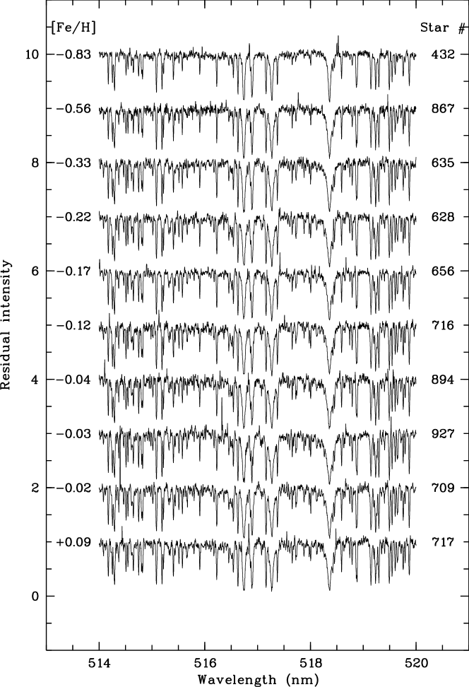
Figure 1: Coadded UVES spectra of the 10 Sgr giants analysed in this paper. The labels on the right denote the star number, those on the left the [FeI/H].

Table 2: Lines

Ion	$\lambda$	log gf	source of	EW	$\epsilon$	EW	$\epsilon$	EW	$\epsilon$	EW	$\epsilon$	EW	$\epsilon$
	(nm)		log gf	(pm)		(pm)		(pm)		(pm)		(pm)
			(see notes)	432		628		635		656		709
Fe I	489.2871	-1.29	FMW	4.42	6.69	8.28	7.34	–	–	7.78	7.44	7.84	7.47
Fe I	506.7151	-0.97	FMW	–	–	10.51	7.41	8.42	7.03	9.54	7.46	9.52	7.49
Fe I	510.4436	-1.69	FMW	2.46	6.72	–	–	4.51	7.14	4.81	7.35	6.28	7.62
Fe I	510.9650	-0.98	FMW	6.07	6.82	–	–	9.51	7.34	7.98	7.24	10.0	7.69
Fe I	552.5539	-1.33	FMW	3.51	6.52	7.17	7.16	8.14	7.30	7.92	7.45	7.43	7.37
Fe I	585.5091	-1.76	FMW	–	–	–	–	–	–	–	–	5.02	7.76
Fe I	585.6083	-1.64	FMW	2.38	6.63	6.16	7.38	5.52	7.23	4.85	7.28	6.61	7.57
Fe I	585.8779	-2.26	FMW	–	–	2.56	7.30	2.88	7.30	2.00	7.24	1.78	7.14
Fe I	586.1107	-2.45	FMW	–	–	–	–	–	–	–	–	2.84	7.66
Fe I	587.7794	-2.23	FMW	1.65	6.88	–	–	–	–	3.64	7.53	4.44	7.64
Fe I	588.3813	-1.36	FMW	5.80	6.70	10.41	7.38	–	–	8.48	7.26	8.85	7.35
Fe I	615.1617	-3.23	FMW	6.81	6.66	9.92	7.04	–	–	9.37	7.22	8.66	7.06
Fe I	616.5361	-1.55	FMW	4.19	6.75	–	–	6.22	7.06	6.39	7.27	6.64	7.30
Fe I	618.7987	-1.72	FMW	4.01	6.65	–	–	7.51	7.20	6.49	7.22	8.42	7.56
Fe I	649.6469	-0.57	FMW	3.56	6.39	9.10	7.29	7.73	7.07	7.81	7.24	9.40	7.54
Fe I	670.3568	-3.16	FMW	4.09	6.67	7.53	7.23	6.29	7.00	7.27	7.37	–	–
Fe II	483.3197	-4.78	FMW	1.20	6.76	–	–	–	–	3.18	7.49	3.50	7.61
Fe II	492.3927	-1.32	FMW	14.99	6.50	–	–	–	–	–	–	–	–
Fe II	499.3358	-3.65	FMW	4.10	6.61	8.35	7.50	6.35	7.04	7.05	7.30	7.35	7.48
Fe II	510.0664	-4.37	FMW	2.08	6.82	3.76	7.38	4.30	7.41	3.30	7.26	3.41	7.34
Fe II	513.2669	-4.18	FMW	2.57	6.76	4.43	7.32	4.01	7.16	4.72	7.36	3.81	7.24
Fe II	516.1184	-4.48	K88	–	–	–	–	–	–	2.17	7.15	–	–
Fe II	525.6938	-4.25	K88	2.57	6.93	5.44	7.67	3.36	7.19	4.66	7.51	3.73	7.39
Fe II	526.4812	-3.19	FMW	4.84	6.79	7.10	7.28	–	–	–	–	7.16	7.43
Fe II	614.9258	-2.72	K88	3.69	6.81	–	–	3.55	6.81	–	–	5.67	7.38
Mg I	552.8405	-0.620	LZ	–	–	21.74	7.09	22.55	7.07	19.77	7.09	21.53	7.20
Mg I	571.1088	-1.833	LZ	7.98	6.75	12.46	7.29	10.81	7.06	11.05	7.27	10.66	7.20
Mg I	631.8717	-1.981	FF	2.08	6.73	5.04	7.32	5.83	7.40	3.59	7.16	5.95	7.51
Mg I	631.9237	-2.201	FF	–	–	4.77	7.50	3.66	7.28	–	–	3.61	7.35
Si I	577.2146	-1.750	GARZ	–	–	–	–	–	–	–	–	4.82	7.22
Si I	594.8541	-1.230	GARZ	6.16	6.79	8.42	7.18	8.26	7.12	9.30	7.38	8.84	7.35
Si I	612.5021	-1.540	ED	1.80	6.83	–	–	–	–	–	–	–	–
Si I	614.2483	-1.480	ED	–	–	4.54	7.45	3.21	7.17	3.50	7.28	4.34	7.46
Si I	614.5016	-1.430	ED	1.39	6.59	–	–	3.28	7.13	3.34	7.20	3.79	7.30
Si I	615.5134	-0.770	ED	3.27	6.42	8.26	7.30	5.64	6.88	7.99	7.32	7.87	7.34
Ca I	551.2980	-0.290	NBS	5.48	5.06	10.74	5.79	10.64	5.80	10.69	6.01	10.47	5.96
Ca I	585.7451	0.230	NBS	–	–	–	–	14.22	5.86	–	–	17.63	6.51
Ca I	586.7562	-1.610	ED	–	–	3.86	6.08	3.22	5.92	4.26	6.26	4.68	6.28
Ca I	612.2217	-0.409	NBS	–	–	–	–	19.53	5.95	–	–	19.51	6.25
Ca I	616.1297	-1.020	NBS	5.98	5.38	–	–	9.33	5.81	9.98	6.12	10.46	6.19
Ca I	616.6439	-0.900	NBS	6.75	5.40	10.81	5.89	9.54	5.72	9.73	5.96	10.29	6.03
Ca I	616.9042	-0.550	NBS	7.25	5.15	13.05	5.88	10.88	5.60	11.64	5.94	12.11	6.01
Ca I	643.9075	0.470	NBS	–	–	–	–	17.94	5.67	–	–	18.91	6.07
Ca I	645.5558	-1.350	NBS	–	–	8.98	6.05	8.05	5.92	8.16	6.13	8.02	6.07
Ca I	649.3781	0.140	NBS	–	–	–	–	15.03	5.57	–	–	–	–
Ca I	649.9650	-0.590	NBS	7.69	5.27	–	–	10.91	5.62	10.92	5.82	12.82	6.15
Ca I	650.8850	-2.110	NBS	1.38	5.46	2.48	5.83	–	–	2.01	5.82	2.31	5.83
Ca I	679.8479	-2.320	K88	–	–	–	–	–	–	1.45	6.05	–	–
ED Edvardsson, B. et al. 1993, A. and A. 275, 101
FF Froese Fischer, C. 1975, Can.J.Phys. 53, 184; p. 338; 1979, JOSA 69, 118.
FMW Fuhr, J.R., Martin, G.A., and Wiese, W.L. 1988. J.Phys.Chem.Ref.Data 17, Suppl. 4.
GARZ Garz, T. 1973, a. and A. 26, 471.
K88 Kurucz, R.L. 1988, Trans. IAU, XXB, M. McNally, ed., Dordrecht: Kluwer, 168-172.
KZ Kwiatkowski, M., Zimmermann, P., Biemont, E., and Grevesse, N. 1982, A. and A. 112, 337-340.
LZ Lincke, R. and Ziegenbein, G. 1971, Z. Phyzik, 241, 369.
NBS Wiese, W.L., Smith, M.W., and Glennon, B.M. 1966, NSRDS-NBS 4.

Table 2: Lines (continued)

Ion	$\lambda$	log gf	source of	EW	$\epsilon$	EW	$\epsilon$	EW (pm)	$\epsilon$	EW	$\epsilon$	EW	$\epsilon$
	(nm)		log gf	(pm)		(pm)		(pm)		(pm)		(pm)
			(see notes)	716		717		867		894		927
Fe I	489.2871	-1.29	FMW	8.67	7.45	7.21	7.50	6.89	7.14	8.21	7.57	7.10	7.44
Fe I	506.7151	-0.97	FMW	11.31	7.59	–	–	–	–	8.82	7.37	9.00	7.56
Fe I	510.4436	-1.69	FMW	–	–	6.32	7.75	5.12	7.23	–	–	5.90	7.62
Fe I	510.9650	-0.98	FMW	8.58	7.20	8.94	7.67	8.06	7.02	9.39	7.59	8.38	7.50
Fe I	552.5539	-1.33	FMW	8.83	7.46	7.41	7.52	6.75	7.04	7.06	7.30 .	6.92	7.38
Fe I	585.5091	-1.76	FMW	–	–	–	–	–	–	4.65	7.69	4.09	7.63
Fe I	585.6083	-1.64	FMW	–	–	5.86	7.57	5.15	7.16	6.89	7.64	6.50	7.66
Fe I	585.8779	-2.26	FMW	2.89	7.41	2.97	7.52	–	–	2.68	7.34	1.91	7.18
Fe I	586.1107	-2.45	FMW	1.60	7.35	2.85	7.75	–	–	2.47	7.56	2.49	7.60
Fe I	587.7794	-2.23	FMW	3.73	7.48	–	–	1.77	6.96	–	–	3.94	7.58
Fe I	588.3813	-1.36	FMW	10.38	7.42	9.18	7.63	6.13	6.65	9.33	7.47	–	–
Fe I	615.1617	-3.23	FMW	10.86	7.26	–	–	8.04	6.73	–	–	9.05	7.27
Fe I	616.5361	-1.55	FMW	–	–	7.64	7.65	4.27	6.75	6.58	7.28	6.14	7.29
Fe I	618.7987	-1.72	FMW	8.21	7.38	6.80	7.41	4.92	6.79	6.74	7.25	6.69	7.33
Fe I	649.6469	-0.57	FMW	8.50	7.23	8.07	7.46	5.75	6.73	9.06	7.51	7.66	7.35
Fe I	670.3568	-3.16	FMW	7.80	7.32	7.83	7.66	7.00	7.10	7.61	7.37	8.36	7.64
Fe II	499.3358	-3.65	FMW	7.14	7.25	6.32	7.27	6.96	6.99	5.78	7.21	5.47	7.33
Fe II	510.0664	-4.37	FMW	4.64	7.51	4.13	7.49	3.63	7.11	4.34	7.60	–	–
Fe II	513.2669	-4.18	FMW	4.64	7.32	4.16	7.30	4.66	7.11	4.67	7.49	3.34	7.34
Fe II	516.1184	-4.48	K88	–	–	–	–	–	–	2.46	7.31	2.12	7.35
Fe II	525.6938	-4.25	K88	–	–	5.06	7.67	–	–	2.93	7.24	3.20	7.46
Fe II	526.4812	-3.19	FMW	–	–	7.55	7.53	6.11	6.85	6.32	7.33	5.27	7.28
Fe II	614.9258	-2.72	K88	5.80	7.25	7.29	7.70	–	–	4.80	7.26	–	–
Mg I	552.8405	-0.620	LZ	21.90	7.14	–	–	17.65	6.71	19.47	7.03	19.47	7.02
Mg I	571.1088	-1.833	LZ	11.76	7.24	12.42	7.59	10.73	7.05	10.49	7.16	11.73	7.40
Mg I	631.8717	-1.981	FF	4.53	7.27	5.34	7.49	2.40	6.83	5.32	7.40	4.97	7.37
Mg I	631.9237	-2.201	FF	–	–	3.78	7.44	2.28	7.02	–	–	–	–
Si I	577.2146	-1.750	GARZ	–	–	–	–	–	–	–	–	4.82	7.30
Si I	594.8541	-1.230	GARZ	10.26	7.44	10.14	7.62	6.71	6.83	9.24	7.45	8.98	7.49
Si I	612.5021	-1.540	ED	–	–	–	–	4.70	6.82	–	–	–	–
Si I	614.2483	-1.480	ED	3.31	7.23	3.64	7.34	3.87	7.24	4.80	7.56	3.63	7.40
Si I	614.5016	-1.430	ED	–	–	4.44	7.43	3.30	7.09	4.83	7.51	4.21	7.46
Si I	615.5134	-0.770	ED	7.01	7.11	8.88	7.55	5.99	6.87	8.67	7.51	7.88	7.46
Ca I	551.2980	-0.290	NBS	11.31	5.99	11.47	6.33	8.98	5.52	10.24	5.92	12.62	6.38
Ca I	585.7451	0.230	NBS	15.84	6.08	–	–	–	–	–	–	–	–
Ca I	586.7562	-1.610	ED	–	–	4.19	6.30	4.00	6.04	5.12	6.32	4.98	6.33
Ca I	616.1297	-1.020	NBS	9.85	5.93	10.93	6.50	8.16	5.62	10.72	6.23	8.64	5.92
Ca I	616.6439	-0.900	NBS	9.91	5.82	10.05	6.21	7.21	5.36	10.42	6.05	9.61	5.99
Ca I	616.9042	-0.550	NBS	11.75	5.75	11.00	6.05	–	–	–	–	11.73	6.05
Ca I	645.5558	-1.350	NBS	8.84	6.09	7.95	6.24	8.75	6.030	9.46	6.30	9.08	6.34
Ca I	649.9650	-0.590	NBS	11.51	5.72	11.51	6.16	–	–	11.53	5.92	12.37	6.20
Ca I	650.8850	-2.110	NBS	3.29	6.04	3.21	6.13	–	–	–	–	2.90	5.93
Ca I	679.8479	-2.320	K88	–	–	–	–	–	–	–	–	1.79	6.06
ED Edvardsson, B. et al. 1993, A. and A. 275, 101
FF Froese Fischer, C. 1975, Can.J.Phys. 53, 184; p. 338; 1979, JOSA 69, 118.
FMW Fuhr, J.R., Martin, G.A., and Wiese, W.L. 1988. J.Phys.Chem.Ref.Data 17, Suppl. 4.
GARZ Garz, T. 1973, a. and A. 26, 471.
K88 Kurucz, R.L. 1988, Trans. IAU, XXB, M. McNally, ed., Dordrecht: Kluwer, 168-172.
KZ Kwiatkowski, M., Zimmermann, P., Biemont, E., and Grevesse, N. 1982, A. and A. 112, 337-340.
LZ Lincke, R. and Ziegenbein, G. 1971, Z. Phyzik, 241, 369.
NBS Wiese, W.L., Smith, M.W., and Glennon, B.M. 1966, NSRDS-NBS 4.

Table 3: Coordinates and atmospheric parameters

Stara	$\alpha(2000)^{b}$			$\delta(2000)^{b}$			$V\leavevmode\nobreak\ (V-I)_{0}^{c}$		$\rm T_{eff}$	log g	$\xi$
432	18	53	50.75	$-30$	27	27.3	17.55	0.965	4818	2.30	1.3
628	18	53	47.91	$-30$	26	14.5	18.00	0.928	4904	2.50	2.0
635	18	53	51.05	$-30$	26	48.3	18.01	0.954	4843	2.50	1.8
656	18	53	45.71	$-30$	25	57.3	18.04	0.882	5017	2.50	1.6
709	18	53	38.73	$-30$	29	28.5	18.09	0.917	4930	2.50	1.5
716	18	53	52.97	$-30$	27	12.8	18.10	0.902	4967	2.50	2.0
717	18	53	48.05	$-30$	29	38.1	18.10	0.872	5042	2.50	1.3
772d	18	53	48.13	$-30$	32	0.8	18.15	0.947	4891	2.50	1.5
867	18	53	53.02	$-30$	27	29.2	18.30	0.933	4892	2.50	2.0
879e	18	53	48.59	$-30$	30	48.7	18.33	0.965	4891	2.50	1.4
894	18	53	36.84	$-30$	29	54.1	18.34	0.940	4876	2.50	1.4
927	18	53	51.69	$-30$	26	50.7	18.39	0.937	4880	2.75	1.2

^a see note to Table 4 ^b accurate to 0$\aas@@fstack{\prime\prime}$3 (Ferraro & Monaco 2002, private communication) ^c The adopted reddening is $E(V-I)=0.22$ ^d this is star [BHM2000] 143 of Bonifacio et al. (2000) ^e this is star [BHM2000] 139 of Bonifacio et al. (2000)

Table 4: Abundances

Stara	S/N	A(FeI)	$n$	A(FeII)	$n$	A(Mg)	$n$	A(Si)	$n$	A(Ca)	$n$
	@530nm
Sun		7.50		7.50		7.58		7.55		6.36
432	28	$6.67\pm 0.12$	12	$6.75\pm 0.13$	8	$6.74\pm 0.01$	2	$6.66\pm 0.16$	4	$5.29\pm 0.14$	6
628	37	$7.28\pm 0.11$	9	$7.43\pm 0.14$	5	$7.30\pm 0.15$	4	$7.31\pm 0.11$	3	$5.92\pm 0.11$	6
635	19	$7.17\pm 0.12$	10	$7.13\pm 0.19$	5	$7.20\pm 0.14$	4	$7.08\pm 0.12$	4	$5.77\pm 0.13$	11
656	24	$7.33\pm 0.10$	14	$7.35\pm 0.13$	6	$7.17\pm 0.08$	3	$7.29\pm 0.07$	4	$6.01\pm 0.14$	9
709	41	$7.48\pm 0.20$	15	$7.41\pm 0.11$	7	$7.31\pm 0.13$	4	$7.34\pm 0.08$	5	$6.12\pm 0.17$	11
716	36	$7.38\pm 0.11$	12	$7.33\pm 0.11$	4	$7.22\pm 0.05$	3	$7.26\pm 0.14$	3	$5.92\pm 0.14$	8
717	20	$7.59\pm 0.10$	12	$7.49\pm 0.16$	6	$7.51\pm 0.06$	3	$7.49\pm 0.11$	4	$6.24\pm 0.13$	8
867	20	$6.94\pm 0.19$	12	$7.13\pm 0.11$	4	$6.89\pm 0.14$	4	$7.00\pm 0.17$	5	$5.72\pm 0.28$	5
894	34	$7.46\pm 0.14$	13	$7.35\pm 0.13$	7	$7.20\pm 0.15$	3	$7.51\pm 0.04$	4	$6.12\pm 0.17$	6
927	43	$7.47\pm 0.15$	15	$7.35\pm 0.06$	5	$7.26\pm 0.17$	3	$7.42\pm 0.07$	5	$6.12\pm 0.17$	9
a Star numbers are from Marconi et al. (1998) field 1, available through CDS
at cdsarc.u-strasbg.fr/pub/cats/J/A+A/330/453/sagit1.dat

3 Analysis

Our analysis was performed on the spectra reduced with the UVES pipeline delivered together with the raw data. Our previous experience (Bonifacio et al., 2002) has shown that the quality of this data is adequate for the determination of abundances. The observed radial velocity of each spectrum was measured by cross-correlation with a synthetic spectrum. This was done independently for both spectral ranges, corresponding to the two CCDs of the mosaic, and was always consistent between the two CCDs. The spectra were then doppler shifted to rest wavelength and different spectra of the same star were rebinned to the same wavelength step and coadded. The resulting S/N ratio of the coadded spectra is in the range 19 – 43 at 530 nm and greater at longer wavelengths. The equivalent widths listed in Table 2 of individual lines were measured using the iraf task splot, either by fitting a single gaussian or multiple gaussians when the lines were slightly blended. The standard deviation of repeated measurement of the same line was of the order of the error estimated from the Cayrel formula (Cayrel, 1988), as expected.

The effective temperatures listed in Table 3 were derived from the $(V-I)_{0}$ colour through the calibration of Alonso, Arribas, & Martínez-Roger (1999), we adopted the reddening $E(V-I)=0.22$, $A_{V}=0.55$ and a distance modulus $m-M=16.95$ from Marconi et al. (1998). For each star we computed a model atmosphere using version 9 of the ATLAS code (Kurucz, 1997) with the above $T\rm_{eff}$ and log g = 2.5, which was estimated from the location of the stars in the $(V-I)_{0},M_{v}$ diagram and the isochrones of Straniero, Chieffi, & Limongi (1997) of ages between 8 and 10Gyr, which is an age range compatible with the anaysis of Marconi et al. (1998). The abundances were determined using the WIDTH code (Kurucz, 1997) except for oxygen; since the only oxygen indicator available is the [OI] 630nm line, which is blended with the Ni I 630.034 nm line we used spectrum synthesis with the SYNTHE code (Kurucz, 1997). For this blending line we used the recently measured log gf = –2.11 of Johansson et al. (2003), and assumed that Ni scales with Fe. We re-determined the oxygen abundance also for star # 772 and the upper limit for # 879, already studied by Bonifacio et al. (2000), with this new log gf for the Ni I line. The model atmospheres were computed switching off the overshooting option, according to the prescription of Castelli, Gratton, & Kurucz (1997) and an opacity distribution function (ODF) with microturbulent velocity $\xi=1$ $\mathrm{kms}^{-1}$, suitable metallicity and [$\alpha$/Fe]= 0.0 or +0.4, adjusted iteratitively in the course of the analysis.

For two stars we decided, in the course of the analysis, to change the surface gravity in order to have a better Fe I /Fe II ionization equilibrium. The new gravity is consistent with the position of the stars in the colour magnitude diagram. Several stars turn out to have solar metallicity and [$\alpha$/Fe]$<$0. Since the effect of different [$\alpha$/Fe] ratios on the temperature structure of model-atmospheres is higher at higher metallicities, our computations, performed with models computed with ODFs with [$\alpha$/Fe]=0., are inconsistent. Fiorella Castelli kindly computed at our request an ODF with solar metallicity and [$\alpha$/Fe] =–0.2 using the same input data as in Castelli & Kurucz (2002) and we computed models using this new ODF. The effect of the new models on our derived abundances was tiny, of the order of a few hundredths of dex. This is due to the fact that the lines we employ are either of medium strength or strong and are therefore formed in rather superficial layers. The difference in structure due to different [$\alpha$/Fe] ratios is strongest at large depths, so that only abundances derived from very weak lines should be affected.

The results of our analysis are summarized in Table 4. In Table 6 we provide the [X/Fe] ratios for all of the Sgr giants observed with UVES, thus including also the two stars from Bonifacio et al. (2000).

The O abundance depends also on the, presently unknown, C abundance, since a significant fraction of O is locked as CO. We assumed [C/Fe]=0.0 . For carbon abundances in the range $-0.5\leq$ [C/Fe]$\leq+0.5$ the effect on the derived O abundance is of the order of 0.01 dex and may therefore be neglected. We may exclude significant ($>0.5$dex) C enhancement, since our spectrum synthesis suggests we would detect some CN lines; this is in agreement with Bonifacio & Caffau (2003), whose automatic code did not flag any of the stars as “suspect CN”. We cannot exclude the C-starved case ([C/Fe]$\la-2.0$), which could be observed in giant stars if the surface material has been polluted by CN cycled material in which C has been depleted. In Galactic globular clusters carbon abundances are in fact usually found below their oxygen abundances (Brown et al., 1990). However the C-starved case would imply lower [O/Fe] ratios of at most 0.2 dex. Since the hypothesis [C/Fe]=0.0 provides [O/Fe] ratios which are in line with the ratios of other $\alpha$ elements to iron, we think it is a reasonable working hypothesis. Furthermore it is extremely unlikely that all stars in the sample are C-starved stars. When C abundances will be derived for these stars the O abundances might be re-considered.

In order to provide a reference for differential metallicities, if desired, we determined the Fe abundance for two giants in the Hyades: HD 27371 and HD 27697. These stars are almost twins and have atmospheric parameters close to those of the Sgr stars analysed in the present paper. A differential metallicity with respect to these should therefore be independent of our adopted temperature scale, model atmospheres and atomic data. We measured equivalent widths on the FEROS spectra for 12 Fe I and 1 Fe II lines out of those in Table 2. There could be some concern in comparing equivalent widths measured with two different spectrographs, of slightly different resolution. However scattered light is known to be very low in both spectrographs and we believe this to be a minor problem (Kaufer & Pasquini, 1998).

We used the measurements of Johnson et al. (1966), as reported in the General Catalog of Photometric data (Mermillod et al., 1996), which imply $V-I=1.20$ for both stars, and a zero reddening, to derive an effective temperature of 4880 K for both stars. We assumed log g = 2.50, like for our program stars and computed a model atmosphere with these parameters, solar metallicity and microturbuence of 1 kms^-1. The derived [Fe/H] is reported in Table 7 together with other determinations for the two stars found in the catalog of Cayrel de Strobel, Soubiran, & Ralite (2001). Our determination is compatible, within errors with all previous determinations. It is interesting to notice that with our parameters the two stars have the same [Fe/H], as is expected from the similarity of the two spectra. The FeI/FeII ionization balance is achieved within errors, for our adopted gravity, albeit Fe II is represented by a single line.

The line to line scatter provided in Table 4 provides a good estimate of the statistical error arising from the noise in our spectra and uncertainties in the measurement of equivalent widths; the errors in the mean abundance may be estimated assuming that each line provides an independent measure of the abundance and dividing the the dispersion by $\sqrt{n}$, where $n$ is the number of measured lines. To this one should add linearly the errors arising from the uncertainties in the atmospheric parameters. As a representative star we take star # 628 and report in Table 5 these errors.

Table 5: Errors in the abundances of star # 628 due to uncertainties in the atmospheric parameters

	$\Delta$A(FeI)	$\Delta$A(FeII)	$\Delta$A(O)	$\Delta$A(MgI)	$\Delta$A(SiI)	$\Delta$A(CaI)
$\Delta\xi=\pm 0.2$ $\mathrm{kms}^{-1}$	${}^{-0.06}_{+0.07}$	${}^{-0.04}_{+0.05}$	$\mp 0.05$	$\mp 0.04$	${}^{-0.03}_{+0.04}$	${}^{-0.05}_{+0.06}$
$\rm\Delta T_{eff}=\pm 100$ K	${}^{+0.14}_{-0.06}$	${}^{-0.06}_{+0.12}$	$\mp 0.01$	${}^{+0.09}_{-0.06}$	${}^{+0.00}_{-0.05}$	${}^{+0.17}_{-0.10}$
$\Delta\log g=\pm 0.50$	${}^{+0.05}_{-0.03}$	${}^{+0.29}_{-0.20}$	${}^{+0.25}_{-0.24}$	${}^{-0.03}_{+0.01}$	${}^{+0.11}_{-0.06}$	${}^{-0.03}_{+0.01}$

Table 6: Abundance ratios

Stara	[Fe/H]	[O/FeII]	[Mg/Fe]	[Si/Fe]	[Ca/Fe]
432	$-0.83\pm 0.12$	$+0.01$	$-0.01$	$-0.06$	$-0.24$
628	$-0.22\pm 0.11$	$-0.16$	$-0.06$	$-0.02$	$-0.22$
635	$-0.33\pm 0.12$	$-0.02$	$-0.05$	$-0.14$	$-0.26$
656	$-0.17\pm 0.10$	$-0.18$	$-0.24$	$-0.09$	$-0.18$
709	$-0.02\pm 0.20$	$-0.14$	$-0.25$	$-0.21$	$-0.22$
716	$-0.12\pm 0.11$	$-0.16$	$-0.24$	$-0.17$	$-0.32$
717	$+0.09\pm 0.11$	$-0.09$	$-0.16$	$-0.15$	$-0.21$
772b	$-0.21\pm 0.19$	$-0.11$	$-0.23$	$-0.07$	$-0.26$
867	$-0.56\pm 0.19$	$-0.01$	$-0.13$	$+0.01$	$-0.08$
879c	$-0.28\pm 0.16$	$\leq 0.18$	$-0.05$	$-0.07$	$-0.21$
894	$-0.04\pm 0.14$	$+0.11$	$-0.34$	$+0.00$	$-0.20$
927	$-0.03\pm 0.15$	$-0.09$	$-0.29$	$-0.10$	$-0.20$

^a see note to Table 4

^b this is star [BHM2000] 143 of Bonifacio et al. (2000)

^c this is star [BHM2000] 139 of Bonifacio et al. (2000)

Figure 2: The metallicity distribution of the 10 Sgr giants of the present paper and the two of Bonifacio et al. (2000)

Table 7: Iron abundances of two Hyades giants

HD 27371						HD 27697
Ref.	$T\rm_{eff}$	log g	$\xi$	[FeI/H]	[FeII/H]	Ref.	$T\rm_{eff}$	log g	$\xi$	[FeI/H]	[FeII/H]
1	4880	2.50	1.3	$+0.21\pm 0.13$	+0.15	1	4880	2.50	1.4	$+0.23\pm 0.13$	+0.05
2	5143	3.02		+0.07		2	5143	2.98		+0.08
3	5040	2.58		+0.17		3	5040	2.44		+0.41
4	5663	2.0		$-0.26$		4
5	4271	3.0		+0.34		5	4235	3.0		+0.30
6	4990	2.80		+0.20		6
7	4800	2.60		+0.09		7
8	4930	2.90		$-0.02$		8	4940	2.85		+0.00
9	4900	2.60		+0.13		9	4875	2.40		+0.06
10	4965	2.65		$+0.15\pm 0.03$

(1) This paper, (2) Lambert & Ries (1981), (3) Gratton et al. (1982), (4) Komarov & Shcherbak (1980), (5) Komarov et al. (1985), (6) Gratton & Ortolani (1986), (7) Fernandez-Villacanas et al. (1990), (8) McWilliam (1990), (9) Luck & Challener (1995), (10) Smith (1999)

4 Metallicity distribution

The histogram of the [Fe/H] for the 12 stars observed with UVES is shown in Fig. 2. In spite of the small number of stars two features are obvious: 1) the bulk of the population is metal-rich with $\rm-0.5\la[Fe/H]\la 0.0$; 2) the spread is of the order of 1 dex.

It is clear that it is not easy to evaluate the relative contribution of each metallicity bin to the total population of Sgr from a sample of only 12 stars. Here and in the rest of the paper we call “dominant population” the one which seems to dominate in Fig. 2, i.e. the stars with [Fe/H]$>-0.5$. When accurate metallicities for a larger number of stars become available it will be interesting to see if the picture which emerges from this small sample will persist.

Our results are somewhat at odds with some of the photometric estimates of these quantities. In Fig. 3 we show the colour-magnitude diagram (CMD) for the field, where our stars were selected, from Marconi et al. (1998). The 12 stars observed with UVES are highlighted as bigger filled symbols. These stars sample the RGB at roughly constant luminosity, spanning all of its width. From this plot it seems likely that, in spite of its limited size, our sample captures the whole metallicity spread in this field of Sgr. We may estimate the corresponding spread in $Z$: our measures indicate that O traces the other $\alpha$ elements and we assume C and N trace Fe, then for our program stars we find $0.002\la Z\la 0.014$. Note, that because of the lack of enhancement of $\alpha$ elements, even the stars with $\rm[Fe/H]\sim 0.0$ have a $Z$ which is slightly sub-solar. In Fig. 3 also two Padova isochrones (Girardi et al., 2002) for the $Z$ values relevant to the program stars are shown. Two things are worth noting:

1. to reproduce the observed RGB of Sgr with isochrones of this high $Z$ very young ages, of the order of 0.5 to 1.0 Gyr, are required

2. the ”blue plume”, which is obvious in the CMD, occupies the same region in the CMD as the Main Sequence and Turn-Off of this metal-rich population.

If the ”blue plume” did not exist, the extremely young age we suggest for the dominant population of this region of Sgr, would not be supported. Instead the fact that this explains a feature of the CMD, which we were not seeking to explain, reinforces our interpretation. A possible problem is that there seem to be too few blue stars to explain all of the RGB stars at $M_{V}\sim 0.9$. A full model population study of the CMD of Sgr is beyond the scope of this paper, as is a precise determination of the age(s) of the metal-rich population of Sgr. In any case, in the interpretation of the CMD, one will have to take into account also:

1. possible incompleteness of the photometry at the luminosity of the “blue plume”;

2. contamination at the apparent luminosity of the RGB by the Bulge and the Galactic disc;

3. the fact that if several populations of different ages are present each will contribute some stars at $M_{V}\sim 0.9$.

The young age of the Sgr dominant population also explains the disagreement in metallicity spread and mean metallicity between the spectroscopic analysis and the photometric estimate. Marconi et al. (1998) compared the CMD shown in Fig. 3 with the fiducial lines of two Galactic Globular Clusters: 47 Tuc and M2. The age of M2 is 2 Gyr older than that of M3 (Lee & Carney, 1999) which is 11.3 Gyr old (Salaris & Weiss, 2002) therefore $\sim 13.3$ Gyr. The age of 47 Tuc is 12.5 Gyr, according to Carretta et al. (2000). Both clusters are representative of an old population. We are thus in presence of a rather extreme case of the well known age–metallicity degeneracy. With our assumed ages and spectroscopic metallicities the morphology of the CMD is well explained by the theoretical isochrones. The high metallicity derived by Bonifacio et al. (2000) raised some concern among several workers in the field. For example Monaco et al. (2002) claimed that the high metallicity derived by Bonifacio et al. (2000) is not representative of the bulk of Sgr and took the metallicity distribution of Smecker–Hane & McWilliam (2002) as being in better agreement with the photometric data. Our results instead reinforce the original findings of Bonifacio et al. (2000). Morever the metallicity distribution found by Smecker–Hane & McWilliam (2002) is quite similar to ours except for the 3 truly metal-poor stars, out of their sample of 14; analogs to these are totally lacking in our sample. It is relevant to point out that Monaco et al. (2002), exactly like Marconi et al. (1998), base their conclusions on comparison with fiducial lines of Galactic Globular Clusters(GGCs). On the other hand Cole (2001), who made use of the slope of the RGB in an IR colour magnitude diagram, arrived at an estimate of [Fe/H]=$-0.5\pm 0.2$ for the bulk of the Sgr population. Quite correctly Cole, pointed out that this estimate could in fact be too low, since the relations are calibrated on GGCs and age effects may bias downwards the results by 0.1-0.2 dex; furthermore the lack of $\alpha-$ enhancement in Sgr (confirmed by the present analysis), at variance with GCCs, would also act in the direction to lower the photometric metallicity estimate.

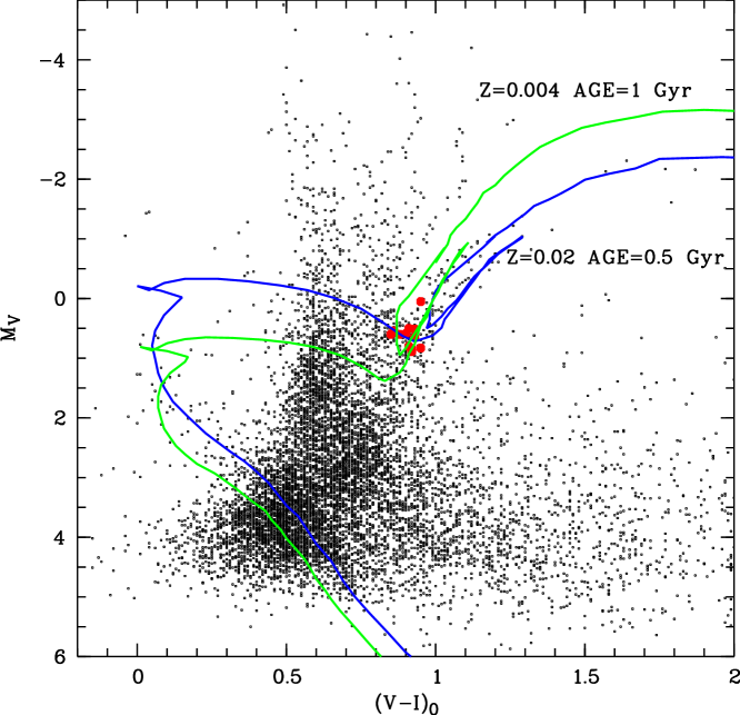
Figure 3: The colour–magnitude diagram of field 1of Marconi et al. (1998), the reddening adopted is $E(V-I)=0.22$ , $A_{V}=0.55$ and the distance modulus $(m-M)=16.95$, from the same reference. The stars observed by UVES are shown with larger symbols, two Padova isochrones (Girardi et al., 2002), covering the range in $Z$ found for the program stars are shown.

Therefore we believe that the high mean metallicity we derive is entirely consistent with extant photometric data, once a young age is allowed for. The real issue, concerning our metallicity distribution, is the lack of the very metal poor population found by Smecker–Hane & McWilliam (2002). For this we see only two possible explanations: either the metal-poor population is not present in the region of Sgr studied by us or our target selection criteria have been such that we missed it.

In the first place it must be borne in mind, that we and Smecker–Hane & McWilliam are sampling both different regions of Sgr and different evolutionary phases. Our stars are bona fide first ascent red giants or clump stars, while the sample of Smecker–Hane & McWilliam quite likely contains also some AGB stars. Unfortunately Smecker–Hane & McWilliam do not provide coordinates for their stars, yet they say that they were selected from the fields imaged by Sarajedini & Layden (1995). These two fields are centered on M54 and 12 arcmin North of the cluster center. On the other hand our stars lie in field 1 of Marconi et al. (1998), which is $\sim 22$ arcmin West of the center of M54. We recall that Marconi et al. (1998) found indeed a difference in colour at the base of the RGB between M54 and field1 and suggested as most likely explanation a difference in mean metallicity of the order of 0.5 dex. We suspect that the metal–poor stars found by Smecker–Hane & McWilliam either belong to M54 or to the neighbouring field (possibly M54 debris) which shares the same metallicity. If this were the case the similarity between the metal–poor stars of Smecker–Hane & McWilliam and the M54 giants investigated by Brown et al. (1999) is not surprising. A possible solution is therefore that the metal-poor population is missing in the region sampled by us.

Inspection of Fig. 3 shows that to the blue of the 1 Gyr isochrone there is an RGB which, if attributed to Sgr, could indeed represent a metal-poor population. In our low-resolution survey, aimed at selecting radial velocity members of Sgr, we ignored that RGB, attributing it to the Bulge. Radial velocity measurements could ascertain if this is the case or if it belongs to Sgr instead. If this were the case then the lack of detection of the metal-poor population can be attributed to our selection of stars to be observed spectroscopically.

The existence of a metal-poor population in Sgr is not questionable, given the results of Brown et al. (1999) for M54, of Smecker–Hane & McWilliam (2002) for the Sgr field. Cseresnjes, Alard, & Guibert (2000) and Cseresnjes (2001) have found RR Lyr variables in Sgr with a period distribution which points towards a mean metallicity, for this old metal-poor population, of [Fe/H]$\sim-1.6$. The real issue is the relative contribution of the various populations and their spatial extents.

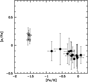
Figure 4: The [Fe/H], [$\alpha$/Fe] diagram for the programme stars (filled symbols. The 5 stars of M54 studied b Brown et al. (1999) are shown as open symbols. [$\alpha$/Fe] in this plot is defined as $1\over 3$([Mg/Fe]+[Si/Fe]+[Ca/Fe]).

Figure 5: The [Fe/H], [$\alpha$/Fe] diagram for the programme stars (filled symbols), the stars in the Local Group dwarf spheoridals, Draco, Ursa Minor, Sextans from Shetrone et al. (2001), Carina, Sculptor, Fornax and Leo from Shetrone et al. (2003) (open circles), Galactic stars from Gratton et al. (2003) (crosses) and for DLAs from Centuriòn et al. (2003) (asterisks). For the stars [$\alpha$/Fe], in this plot, is defined as $0.5\times$([Mg/Fe]+[Ca/Fe]), for the DLAs [Si/Zn] is used as a proxy for [$\alpha$/Fe] and [Zn/H] as a proxy for [Fe/H]

5 $\alpha$/Fe ratios

The ratios of $\alpha$ elements to iron peak elements allow one to place important constraints on the star formation history of a galaxy. The common wisdom is that $\alpha$ elements are synthesized by core collapse SNe, while Fe is synthesized mainly by Type Ia SNe (e.g. Marconi et al., 1994,  and references therein). At early time the gas is enriched by SNeII only, thus the $\alpha$/Fe ratio is that characteristic of the yields of massive stars. As time proceeds the type Ia SNe begin to contribute to the Fe content, lowering the $\alpha$/Fe ratio. In the Milky Way at low metallicities the $\alpha$/Fe ratio is higher than at solar metallicity. As shown in figure 3 of Marconi et al. (1994) a slow, bursting or gasping star formation rate may attain a solar $\alpha$/Fe ratio at considerably lower metallicities, and even reach values lower than the solar ratio.

In Fig. 4 we show the mean [Fe/H], [$\alpha$/Fe] diagram for the programme stars. As [$\alpha$/Fe] we have adopted the straight mean of [Mg/Fe], [Si/Fe] and [Ca/Fe]; oxygen has not been included in the mean since the errors associated are considerably larger than for the other elements, note however that in all cases [O/Fe] is consistent with the above defined [$\alpha$/Fe]. The error on this this ratio was computed by propagating the errors on the various [X/H] ratios involved. The figure provides an indication that the $\alpha$/Fe ratio is below solar, although the errors are such that [$\alpha$/Fe]=0.0 cannot be excluded. What can confidently be excluded is an $\alpha$ enhancement, even at the lowest metallicities observed, which strongly suggests a slow or bursting star formation rate. Low $\alpha$/Fe ratios seem to characterize also the other dwarf spheroidals for which spectroscopic abundance ratios are available (Shetrone et al., 2001, 2003). Also the metal rich part of the sample of Smecker–Hane & McWilliam (2002) shows low $\alpha$/Fe ratios, consistent with ours, within errors. The data of Smecker–Hane & McWilliam gives the impression of an increase of the $\alpha$/Fe ratio with decreasing metallicity, however this impression is driven only by data for the three most metal-poor stars. Our data instead seems very flat, with a very weak trend in $\alpha$/Fe, if any. The 5 stars of M54 studied by Brown et al. (1999), which have [Fe/H]$\sim-1.5$, comparable to the most metal-poor stars found by Smecker–Hane & McWilliam (2002), show a very mild $\alpha$ enhancement, of the order of [$\alpha$/Fe]=+0.2 or lower. When joined with our data (Fig. 4) they suggest a mild increase in $\alpha$/Fe ratio, which is not so evident from our data alone. The $\alpha$ enhancement in M54 seems slightly lower than that measured in the most metal-poor stars of Smecker–Hane & McWilliam (2002), although they are compatible within errors.

In Fig. 5 we assemble together our data for Sgr, the data of Shetrone et al. (2001) for the Local Group dwarf spheoridals Draco, Ursa Minor, Sextans, and of Shetrone et al. (2003) for Carina, Sculptor, Fornax and Leo I , the data of Gratton et al. (2003) on Galactic stars and the data compiled by Centuriòn et al. (2003) for Damped Lyman $\alpha$ systems (DLAs). For all the stars in this plot [$\alpha$/Fe] has been defined as the mean of [Mg/Fe] and [Ca/Fe]. This is different from the definition used in Fig. 4 because most of the stars of Shetrone et al. (2001) and Shetrone et al. (2003) do not have any Si measurement. Comparison of our points in figures 4 and 5 shows that there is little difference in the two definitions of [$\alpha$/Fe]. For the DLAs we have used [Si/Zn] as a proxy for [$\alpha$/Fe] and [Zn/H] as a proxy for [Fe/H], because Zn is unaffected by dust depletion and Si is only mildly depleted in DLAs (Vladilo, 2002; Centuriòn et al., 2003). In the metallicity range relevant to DLAs, Zn tracks Fe in Galactic stars, possibly with a small offset of the order of 0.1 dex(Gratton et al., 2003); we stress that the picture does not change significantly even taking this small offset into account. Figure 5 clearly shows that dSph galaxies and most of DLAs are on a chemical evolutionary path different from that of the Milky Way. There seems to be continuity among the dwarf spheroidals which may suggest that they are all on similar evolutionary paths, but some are more chemically evolved than others. It is also tempting to conclude that most of the DLAs follow a chemical evolution similar to that of the dwarf spheroidals. From there it takes only one more step to conclude that most DLAs are dwarf spheroidals caught when they were still gas-rich. The argument that most of DLAs are characterized by low star formation rate and are therefore dwarf galaxies, has already been put forward by Centuriòn et al. (2000). It receives support from the few imaging studies, which show many of the DLAs to be associated with dwarf galaxies and low surface brightness galaxies (Le Brun et al., 1997; Rao & Turnshek, 1998). However up to now there was no clear observational evidence that the $\alpha$ to iron ratios of dwarf galaxies are indeed similar to those of DLAs, as expected from chemical evolution models (Marconi et al., 1994), Fig. 5 forcefully provides this evidence.

6 A scenario for star formation history in Sgr

We believe that our findings, when joined to the other information we have of Sgr, suggest a well defined star formation scenario, whose viability, however, needs to be verified by hydrodynamical simulations.

Sgr has undergone many star bursts, and each starburst is triggered by the interaction of Sgr with the disc of our Galaxy when Sgr passes through it. The simulations of Ibata & Razoumov (1998) indicate that the HI disc of the Galaxy is shocked and warped by the passage of the dwarf galaxy. Furthermore there is substantial heating in the disc shocks and in the tidal tails which follow the dwarf galaxy. The simulations Ibata & Razoumov are not designed to investigate star formation, however Ng (1998) points out that the number density and temperature of the gas are such that a part of the gaseous material should be converted to stars. It therefore seems plausible that star formation is triggered by the shock both in the Galactic disc and in the dwarf galaxy, if it possesses any gas. Besides it is conceivable that some of the gas may be stripped from the Galaxy and follow Sgr, perhaps forming stars. Dedicated simulations, with a live Halo, rather than the static one used by Ibata & Razoumov, are highly desirable to verify if this scenario is actually viable.

6.1 Carbon stars

According to this scenario the dominant population we see in field 1 was formed when Sgr last passed through the Galactic disc. This scenario has also the virtue of explaining the mystery of the Bulge C stars (Ng, 1997, 1998). The presence of carbon stars in fields of the Bulge has been known for over twenty years (Blanco, Blanco, & McCarthy, 1978; Azzopardi, Lequeux, & Rebeirot, 1988). However if these stars belong to the Bulge they are about 2.5 mag too faint to be on the AGB tip, where the carbon-star phenomenon is believed to take place. Moreover the Bulge population is believed to be old, while for a solar metallicity population the mass of the carbon stars should be greater than 1.2 M☉ and their age younger than 4 Gyr (Marigo, Girardi, & Bressan, 1999). This fact lead Ng to look for an alternate explanation. He noticed that the distance modulus of Sgr is in fact 2.5 mag fainter than that of the Bulge. This implies that, if placed at the distance of the Sgr, the Bulge carbon stars appear to have the theoretically expected luminosity. However the radial velocities of the carbon stars of Azzopardi et al. (1991) does not allow to consider them as members of Sagittarius. On the other hand Sagittarius surely has some carbon which are established radial velocity members stars (Ibata, Gilmore, & Irwin, 1995) and several candidate stars (Whitelock, Irwin, & Catchpole, 1996; Ng & Schultheis, 1997). All these observations are explained quite naturally by the star formation scenario proposed by us: the last crossing of the Galactic disc by Sgr triggered star formation both in Sgr (the metal-rich population and the blue plume) as well as in the Galactic disc; some of these stars evolved to become carbon stars in the disc (which has been disturbed) at a distance from us which is about that of Sgr and these are the stars of Azzopardi et al. (1991) and all the other so-called Bulge carbon stars; the same happened to some stars in Sgr and these are the carbon stars with Sgr membership (Ibata, Gilmore, & Irwin, 1995) and also the other candidate stars, if confirmed (Whitelock, Irwin, & Catchpole, 1996; Ng & Schultheis, 1997). If this is case the difference in J-K colour between the two groups cannot be due to a difference in age, but only to differences in metallicity and reddening.

We note that overdensities of carbon stars in the Halo are one of the main tracers of stellar “streams” ascribed to the disruption of Sgr (Ibata et al., 2001).

6.2 Was there gas in Sgr to support star formation ?

A major problem with this scenario is the lack of any detectable amount of gas in Sgr (Burton & Lockman, 1999). One is forced to admit that during the last passage the star formation and the gas stripping has exhausted all the available gas. If that is so, no star formation shall take place in the next passage, unless Sgr is capable to capture gas from the Galactic disc or to capture intergalactic gas clouds. Such an event has been suggested to be the cause of the present star forming activity in the Magellanic Clouds (Hirashita, 1999; Hirashita, Kamaya, & Mineshige, 1997).

We also wish to point out that a factor that may help Sgr in retaining hot gas, thus providing material suitable for forming the next generation of stars, is the fact that the cooling time is of the order of, or even smaller than, the crossing time. This is due to the high metallicity which makes the line cooling very efficient, as may be deduced by following the treatment of Hirashita (1999) and setting $\zeta=Z/Z_{\odot}=0.7$.

6.3 Similarity with the LMC

There are some important similarities between Sgr and the LMC, which seem to suggest that Sgr was more massive in the past and perhaps its mass was of the order of that of the LMC: 1) the RR Lyr populations of the two galaxies are basically indistinguishable; 2) so is the mean metallicity of the younger populations ([Fe/H]$\sim-0.25$ ); 3) at the intermediate and high metallicities also the LMC shows low $\alpha$/iron ratios (Hill et al. in preparation); 4) the pattern of the abundances of neutron capture elements is similar, as pointed out by Bonifacio et al. (2000).

7 Conclusions

With the 10 stars analysed in this paper, the sample of Sgr giants in field 1 of Marconi et al. (1998) has risen to 12. The dominating population appears to be close to solar metallicity and the metallicity range is $\rm-0.8\la[Fe/H]\la 0.0$. The ratio of $\alpha$ elements to iron is sub-solar or solar even at the lowest metallicity observed. In our sample stars which are as metal-poor as M 54 or the most metal-poor stars in the sample of Smecker–Hane & McWilliam (2002) are missing. Therefore either such very metal-poor component has a very low space density in field 1 , perhaps is even absent, or our selection criterion has totally missed this population. This issue needs to be elucidated by the observation of a larger number of stars in the field which we plan to perform with the FLAMES facility on the VLT (Pasquini et al., 2000, 2002).

Our results raise an important question: why is the most metal-poor population of Sgr observed by us so (relatively) metal rich ? In our opinion there are two most likely mechanisms for this enrichment: 1) the gas has been enriched by previous generations of Sgr stars or 2) the gas out of which stars of Sgr were formed was polluted by SNe in the Milky Way, the pollution process being possibly favoured by the passage of Sgr through the Galactic disc.

Either solution has some problems. In the first case it is not clear where the low-mass stars of the previous generations of Sgr are, nor is it clear how Sgr managed to retain the SNe ejecta in order to attain such a high metallicity. In the second case it is not clear how the pollution may take place; the passage of Sgr through the Galactic disc might offer the opportunity, however the degree of pollution, if any, has still to be evaluated.

Whichever the case we note that the high metallicity we derived places Sgr clearly outside the metallicity - luminosity correlation which seems to hold for other Local Group galaxies (van den Bergh, 1999,  and references therein): Sagittarius is underluminous for its metallicity. The capability of attaining a high metallicity is usually associated with the ability to retain the SNe ejecta and therefore a rather large gravitational potential. We therefore believe that an explanation of the high metallicity associated to a relatively low luminosity must be sought among the following: 1) Sgr posseses an extraordinarily large amount of dark matter ; 2) Sgr was much more massive in the past, during the phase in which it raised its metallicity and has now lost much of its mass due to interaction with the Milky Way; 3) the interaction with the Milky Way, through pollution and/or tidal interaction which resulted in increased star formation activity and ability to retain the SNe ejecta. These are not mutually exclusive and a combination of the above is possible.