Highly Ionized Gas Surrounding High Velocity Cloud Complex C

Abstract

We present Far Ultraviolet Spectroscopic Explorer and Hubble Space Telescope observations of high, intermediate, and low ion absorption in high-velocity cloud Complex C along the lines of sight toward five active galaxies. Our purpose is to investigate the idea that Complex C is surrounded by an envelope of highly ionized material, arising from the interaction between the cloud and a hot surrounding medium. We measure column densities of high-velocity high ion absorption, and compare the kinematics of low, intermediate, and high ionization gas along the five sight lines. We find that in all five cases, the H I and O VI high-velocity components are centered within 20 km s^-1 of one another, with an average displacement of $<\bar{v}_{\mathrm{O~{}VI}}-\bar{v}_{\mathrm{H~{}I}}>=3\pm 12$ km s^-1. In those directions where the H I emission extends to more negative velocities (the so-called high-velocity ridge), so does the O VI absorption. The kinematics of Si II are also similar to those of O VI, with $<\bar{v}_{\mathrm{O~{}VI}}-\bar{v}_{\mathrm{Si~{}II}}>=0\pm 15$ km s^-1. We compare our high ion column density ratios to the predictions of various models, adjusted to account for both recent updates to the solar elemental abundances, and for the relative elemental abundance ratios in Complex C. Along the PG 1259+593 sight line, we measure $N$(Si IV)/$N$(O VI) $=0.10\pm 0.02$, $N$(C IV)/$N$(O VI) $=0.35^{+0.05}_{-0.06}$, and $N$(N V)/$N$(O VI) $<0.07$ (3$\sigma$). These ratios are inconsistent with collisional ionization equilibrium at one kinetic temperature. Photoionization by the extragalactic background is ruled out as the source of the high ions since the path lengths required would make HVCs unreasonably large; photoionization by radiation from the disk of the Galaxy also appears unlikely since the emerging photons are not energetic enough to produce O VI. By themselves, ionic ratios are insufficient to discriminate between various ionization models, but by considering the absorption kinematics as well we consider the most likely origin for the highly ionized high-velocity gas to be at the conductive or turbulent interfaces between the neutral/warm ionized components of Complex C and a surrounding hot medium. The presence of interfaces on the surface of HVCs provides indirect evidence for the existence of a hot medium in which the HVCs are immersed. This medium could be a hot ($T\gtrsim 10^{6}$ K) extended Galactic corona or hot gas in the Local Group.

1 Introduction

Complex C is an extensive high-velocity cloud (HVC) covering 1700 square degrees in the northern Galactic sky and falling at an average LSR velocity of $-130$ km s^-1 onto the Milky Way. Because of its low metallicity ($\approx 0.1-0.2$ solar), Complex C is suspected of comprising either intergalactic gas or material tidally stripped from a nearby galaxy, with perhaps some contribution from upwelling Galactic outflow. HVCs are defined as clouds whose observed radial velocities deviate significantly with those expected from Galactic rotation, corresponding in practice to clouds with $|v_{LSR}|>100$ km s^-1. They have traditionally been studied in neutral hydrogen 21 cm emission, and more recently with both H$\alpha$ emission measurements and absorption line studies.

Until 1995, all the absorption detected in HVCs had been in lines of neutral or low ionization species. Highly ionized gas was then discovered with the detections of high-velocity C IV in the spectra of Mrk 509 and PKS 2155–304 (Sembach et al., 1995, 1999). Following the launch of the Far Ultraviolet Spectroscopic Explorer (FUSE) satellite in the summer of 1999, O VI has been repeatedly detected in absorption in HVCs; the first high-velocity O VI results were reported by Sembach et al. (2000) and Murphy et al. (2000). More recently, a survey of high-velocity O VI has been completed by Sembach et al. (2003a, hereafter S03). Since O VI is an ion that exists at temperatures of a few$\;\times 10^{5}$ K (Sutherland & Dopita, 1993), its presence in HVCs poses a variety of intriguing questions: primarily, what physical process produces the O VI? Does the ion originate at some form of interface between the neutral and warm ionized components of HVCs and a surrounding hot medium? Can photoionization by the hard extragalactic radiation field play an important role? S03 began to address these issues with a study of 102 sight lines, 58 of which displayed high-velocity O VI absorption.

In this project we focus our attention on five extragalactic sight lines (Mrk 279, Mrk 817, Mrk 876, PG 1259+593, and PG 1351+640) passing through HVC Complex C, in order to determine the inter-relationships between the various phases of gas present in HVCs. Our approach is to compare the kinematics and column densities of high and low ion absorption in high-velocity gas. Clues concerning the physical conditions within the absorbing material are provided by observing the extent and structure of the absorption profiles in different species.

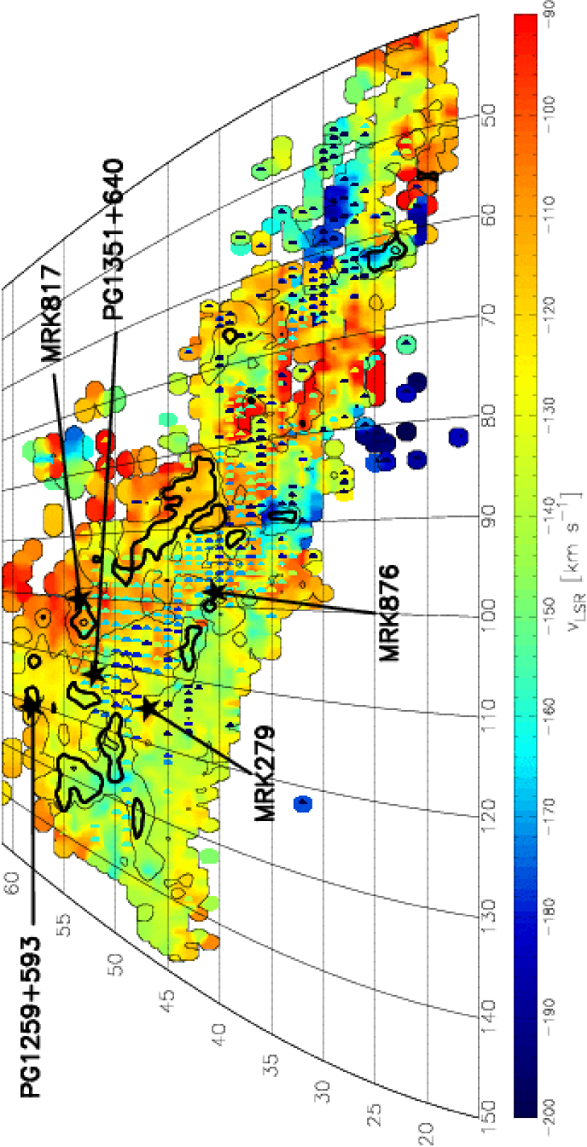
Figure 1: H I velocity field of Complex C, over the range $-200<v_{LSR}<-80$ km s^-1, from the Dwingeloo HVC Survey (Hulsbosch & Wakker, 1988). The survey was completed on a $1\arcdeg\times 1\arcdeg$ grid with a $36\arcmin$ beam, 16  km s^-1 velocity resolution (FWHM) and a 0.05 K detection limit. The sight lines we study in this paper are identified with stars. The contours represent column density levels of $0.2,1.0$ and $3.0\times 10^{19}$ cm^-2. The half circles represent those directions with an additional higher velocity H I component, dubbed the high-velocity ridge.

In Figure 1 we show a color map of Complex C from the Dwingeloo HVC survey (Hulsbosch & Wakker, 1988), displaying the velocity structure within the complex. Gas covering a range in velocities of $\approx 100$ km s^-1 is present in Complex C. The observed range in column densities and velocities indicates a complex system with a large amount of sub-structure. The sight lines studied in this paper are marked with stars.

Our paper is structured as follows: In §2 we give a brief summary of previous studies of Complex C. Section 3 contains a description of our observations and data reduction. We present spectroscopic measurements of high-velocity, highly ionized absorption in §4. In §5 we display our spectra and compare the high and low ion absorption along five Complex C sight lines. In §6 we discuss and review various models that might explain the existence of highly ionized gas in HVCs. In §7 we discuss the influence of non-solar abundance patterns on the model predictions. The theories are compared with our observations in §8, using ionic ratios and kinematic information. We mention interesting results from sight lines passing near to Complex C in §9. Our results are summarized in §10.

2 Previous Studies of Complex C

Detailed abundances studies of Complex C have been carried out by a number of authors (Wakker et al., 1999; Richter et al., 2001a; Gibson et al., 2001; Collins, Shull, & Giroux, 2003a; Tripp et al., 2003; Sembach et al., 2003b), who have all used HST and FUSE spectroscopy to determine column densities of various ionic species through the complex, and combined them with H I 21 cm emission measurements to derive elemental abundances. These studies have found values of (O I/H I) between 0.09 and 0.25 times solar, and no evidence for depletion onto dust. Precise measurements are difficult because of a number of sources of error, particularly uncertain ionization corrections, the difficulty of measuring a precise $b$ value, and the fact that H I radio emission measurements sample a beam far larger than that probed in absorption measurements.

Relative elemental abundance ratios are important in understanding the history of Complex C. Russell & Dopita (1992) find that in the Magellanic Clouds log (N/O)${}_{LMC}=-1.21$ and log (N/O)${}_{SMC}=-1.40$, and Kobulnicky & Skillman (1996) found that log (N/O) typically lies between $-1.7$ and $-1.5$ in dwarf galaxies with log $A_{\mathrm{O}}<-4.0$. An observed value in Complex C is log (N/O)$~{}=-1.7$ (Collins et al., 2003a, towards PG 1259+593), in line with these measurements in other locations.

A conclusive direct distance determination would be an invaluable piece of information in studying Complex C; unfortunately, such a determination is difficult to make. The strongest constraint that exists is a lower limit of 6.1 kpc (Wakker, 2001), based upon the non-detection of Ca II in absorption towards stars at known distances lying in this part of the sky. Note, however, that this non-detection is not strongly significant (as defined by Wakker, 2001). A more reliable lower limit to the distance is 1.3 kpc.

It has been suggested that HVCs may represent material taking part in a Galactic fountain (Shapiro & Field, 1976; Bregman, 1980). However, the low metallicities observed make this scenario unlikely for Complex C, since fountain gas, having been blown out of the disk by Type II supernovae, should have solar or super-solar rather than sub-solar abundances, and a solar N/O ratio of log (N/O)${}_{\odot}=-0.8$. Substantial dilution by primordial gas would be necessary to bring fountain gas down to the observed level of metallicity. We note that the approximately solar abundances measured in intermediate velocity clouds (IVCs; Richter et al., 2001a) suggest they are formed by Galactic material; it is the IVCs that are consequently thought to be tracing the fountain circulation.

3 Observations and Data Reduction

The FUSE satellite (Moos et al., 2000) operates in the far-ultraviolet wavelength regime between 905 and 1187 Å, providing medium resolution ($R\approx 15,000$, corresponding to $\approx 20$ km s^-1 FWHM) spectra with enough sensitivity that faint extragalactic sources can be observed. The FUSE data analyzed in this paper were obtained from the Multimission Archive at the Space Telescope Science Institute (MAST).

In order to investigate the highly ionized gas in Complex C, we took all the sight lines through Complex C observed with the FUSE satellite and applied a set of selection criteria to identify those directions containing useful high ion information. These criteria took the form of a series of constraints, that eventually left us with our sample. To be classified as going through Complex C, we required that a sight line had to lie within the $2\times 10^{18}$ cm^-2 contour of $N$(H I) in the Hulsbosch & Wakker (1988) Dwingeloo HVC survey. Constraint 1 eliminated sight lines with poor signal-to-noise, i.e. S/N$~{}<5$ near 1030 Å in the 10-pixel-rebinned FUSE spectrum. Constraint 2 looked for sight lines with good O VI data, and rejected those with blending or continuum placement problems. Finally, Constraint 3 looked for sight lines that have been observed with either the Goddard High Resolution Spectrograph (GHRS) or the Space Telescope Imaging Spectrograph (STIS) on HST, at better than 30 km s^-1 resolution. Those that were not were eliminated. The reason for Constraint 3 is that with HST data we can form ionic ratios with O VI, or at least upper limits, to investigate the ionization mechanism. Such an approach cannot be achieved with FUSE data alone. Applying these conditions generated our sample of five sight lines, namely Mrk 279, Mrk 817, Mrk 876, PG 1259+593, and PG 1351+640, each of which have good FUSE and HST data. Of our chosen five sight lines, two (Mrk 279 and Mrk 817) have GHRS spectra of the region near 1240 Å, where the N V doublet lies, and three (Mrk 876, PG 1259+593 and PG 1351+640) have STIS spectra covering this region. In the case of PG 1259+593, we were also able to use STIS data of Si IV, C IV, and various low-ionization species. Consequently, this remains the sight line for which we have the best quality data available, and the strongest insight into ionization processes.

A summary of basic target data is given in Table 1, where for each sight line we include Galactic longitude $l$, Galactic latitude $b$, redshift of source $z$, type of source, apparent $B$ magnitude of source, Galactic foreground interstellar reddening $E(B-V)$, high-velocity neutral hydrogen column density $N$(H I), heliocentric to LSR velocity correction $\Delta v_{LSR}$, and recent measurements of [O/H] and [N/H] in Complex C by Collins et al. (2003a).

In the following two subsections we describe our data handling procedures for our two separate datasets.

3.1 FUSE

Details of our FUSE observations are given in Table 2. The data were reduced using the data reduction pipeline CALFUSE v2.1.6, except for Mrk 279, for which we used v2.0.5. This anomaly was because of compatibility problems between early FUSE datasets (such as the Mrk 279 observations) and the newer versions of the CALFUSE pipeline. The difference in velocity calibration caused by this inconsistency is expected to be minimal, since all CALFUSE versions after 2.0 have greatly improved velocity scale accuracy over earlier ones.

Despite the improvements made in the calibration software, we still found it necessary to apply velocity shifts to each spectrum to register the velocity scale correctly. Our approach was to tie the Si II $\lambda 1020.699$, C II $\lambda 1036.337$, O I $\lambda 1039.230$, and Ar I $\lambda 1048.220$ absorption lines to the centers of emission observed in H I, using Effelsberg 100 m radio telescope 21 cm observations. This process transforms the velocity scale into the Local Standard of Rest (LSR) frame. After using Gaussian component fitting software to measure the velocity centroids of components in neutral gas absorption lines, we determined the velocity correction necessary to align these components with the corresponding components seen in H I. Where possible, we tied the scale to the high-velocity components of H I, since these velocities were often cleaner and more distinct, and hence easier to measure. The actual lines used for alignment in each case depended on the individual spectrum. We checked for velocity scale differences between different channels and different exposures within the same channel. The shifts we applied were all in the range 10 to 50 km s^-1. The Effelsberg 100 m radio telescope has a beam size of $9\arcmin\!.7$, and a velocity resolution of $\approx 1$ km s^-1; the H I observations we used are described in detail in Wakker et al. (2001).

Our alignment procedure has the advantage that H I spectra are extremely reliable in their velocity calibration, since radio frequencies can be measured with very high precision. Additionally, when observing an H I spectrum towards an extragalactic source, one has the advantage of knowing that the source is beyond the emitting gas, so absorption lines and emission lines can be reliably compared. Thus the only potential source of errors in our alignment process are the assumptions that the neutral ions trace the H I, and that emission measurements extending over the radio telescope beam of ten arcminutes can be safely compared to absorption measurements sampled over an effectively infinitesimally small beam equal to the angular size of the AGN. In light of these concerns, we estimate an error of 5 km s^-1 in our FUSE velocities after alignment. A detailed discussion of velocity calibration issues in FUSE spectra, and how to deal with them, is given in Wakker et al. (2003).

Since each pixel on the FUSE detectors has a velocity width of $\approx 2$ km s^-1, but the instrumental resolution is only $\approx 20$  km s^-1 (FWHM), the data from the instrument are highly oversampled, and so we have rebinned each spectrum by five pixels (i.e. to $\approx 10$  km s^-1 bins) to obtain the versions displayed and measured in this paper. We fit continua to our spectra using low order ($n=1-3$) Legendre polynomials over $\approx 5$ Å regions on either side of each line under study.

The primary focus of our investigation is O VI $\lambda 1031.926$, since the presence of transition-temperature gas in high-velocity clouds has only recently been discovered. Absorption from C II${}^{*}~{}\lambda 1037.018$ is responsible for blending with high-velocity (Complex C) absorption from the weak O VI line, at 1037.627 Å; we therefore do not include measurements of the weak O VI line in this work. We also study Si II $\lambda 1020.699$, C II $\lambda 1036.337$, and Ar I $\lambda 1048.220$. The C II line is very strong, and although this typically leads to saturation in the line center, the high sensitivity in the wings helps to reveal the full extent of the neutral gas absorption; the H I 21 cm line is not sensitive to these lower column density regions. Unfortunately, we could make no clean observation of C III $\lambda 977.020$, a tracer of intermediate-ionization gas, at Complex C velocities, because the C III line is blended below $-100$ km s^-1 by zero velocity absorption from O I $\lambda 976.448$. The same blending problem afflicts high-velocity absorption by Fe III $\lambda 1122.524$, this time by Fe II $\lambda 1121.975$. Although C III or Fe III are stronger and hence more preferable tracers of intermediate-ionization gas, we do include profiles of S III $\lambda 1012.495$, to trace the kinematics of this phase of interstellar gas.

The strength of contamination from molecular hydrogen varied between our five sight lines. The H₂ (6–0) P(3) line at 1031.191 Å is the offending line, since in the rest frame of O VI $\lambda 1031.926$ it has a velocity of $-213.5$ km s^-1, near the negative velocity limit of Complex C. For Mrk 876, where the H₂ column density is the highest, we corrected the O VI profile for contamination from H₂ by measuring the other H₂ lines in the vicinity of the O VI line. Our model of the H₂ (6–0) P(3) line included two components (1: $v_{LSR}=-7$ km s^-1, depth = 0.60, FWHM = 31 km s^-1; 2: $v_{LSR}=-36$ km s^-1, depth = 0.30, FWHM = 19 km s^-1). The effect of this process is to reduce the measured high-velocity O VI column density slightly. To account for the errors this process introduces, our systematic error on the O VI column density towards Mrk 876 includes the effect of varying the model parameters: $v$(H₂) by $\pm 10$ km s^-1, the H₂ depth by $\pm 10$%, and the H₂ width by $\pm 10$%. Towards PG 1351+640, the sight line with the second highest molecular hydrogen column density, the Complex C O VI absorption does not extend to $-200$ km s^-1, so there is no H₂ interference.

3.2 HST

The GHRS and STIS spectra we use are described in Table 3. We refer the reader to Brandt et al. (1994) and Kimble et al. (1998) for descriptions of the on-orbit performance of the GHRS and STIS instruments, respectively. All data were all taken with intermediate resolution gratings, and were reduced using standard processing pipelines. The grating used and its resolution, found in the GHRS (Soderblom et al., 1995) and STIS (Proffitt et al., 2002) Instrument Handbooks, are listed for each exposure in columns three and eight.

In order to achieve consistency in comparing FUSE and HST spectra, we chose to display all absorption line spectra in 10 km s^-1 bins. Given that the pixel size between GHRS and STIS exposures varies (column nine), our wish for 10 km s^-1 rebinned pixels implied a different rebinning factor for the different HST spectra, and this factor is given in column ten of Table 3.

The velocities were converted from the heliocentric to the LSR reference frame using the corrections listed in Table 1. The velocity calibration from the HST detector pipelines is far more reliable than from the FUSE pipelines, so no further alignment was considered necessary. Any residual errors introduced by inaccuracies in the GHRS and STIS wavelength scales are unlikely to change the conclusions of this paper, since the kinematic inter-relationships we focus on are mainly between absorption lines in the FUSE dataset.

We used $\approx 10$ Å regions on either side of N V $\lambda 1238.821$ for continuum fitting, in the same manner as was used for the FUSE data (§3.1). In the case of PG 1259+593, the same procedure was used for Si IV $\lambda 1393.755$, C IV $\lambda 1548.195$, and various low and intermediate ionization lines. All our targets are extragalactic sources, which tend (unlike stellar spectra) to have flat continua, so the continuum placement process was generally straightforward.

4 Results

Our measurements of high-velocity, highly ionized absorption are presented in Table 4. For each high ionization absorption line detected at Complex C velocities, we list the rest vacuum wavelength ($\lambda$), velocity range of high-velocity absorption ($v_{min}$, $v_{max}$), velocity centroid and width of high-velocity absorption ($\bar{v}$ and $b$), obtained through either the moments of the apparent optical depth profile or through Gaussian component fitting, equivalent width ($W_{\lambda}$), column density ($N$) and signal-to-noise ratio per resolution element (S/N) in the vicinity of the line. All velocities in this table, and throughout this paper, are quoted in the LSR reference frame, and all column densities quoted are measured in the high-velocity gas, not integrated over the full extent of the absorption. S III is not usually recognised as a high ion, but we include measurements of high-velocity S III absorption here to assess the relationship between absorption in intermediate and highly ionized gas.

The velocity ranges we used for the Complex C absorption were chosen after careful consideration of the extent of the high-velocity absorption in different species along each sight line. In some cases these are different (by up to 20 km s^-1) from the velocity ranges used in S03, due to the addition of newer, higher S/N data and improvements in the pipeline processing.

Our table makes use of two methods for finding the central velocity and width of highly ionized absorption. When possible, we fit Gaussian components to the data, and present the formal central velocity ($\bar{v}$) and width ($b$) of the Gaussian. This is only possible when the high-velocity component is distinct and free from blending with other lines. The other method makes use of the moments of the apparent optical depth, found from the continuum-normalized flux profile $F(v)$ by

$$\tau_{a}(v)=\mathrm{ln}\frac{1}{F(v)}.$$ (1)

The first moment gives the velocity centroid

$$\bar{v}=\int^{v_{max}}_{v_{min}}v\tau_{a}(v)\mathrm{d}v/\int^{v_{max}}_{v_{min}}\tau_{a}(v)\mathrm{d}v.$$ (2)

The second moment yields the Doppler width

$$b=\sqrt{2\int^{v_{max}}_{v_{min}}(v-\bar{v})^{2}\tau_{a}(v)\mathrm{d}v/\int^{v_{max}}_{v_{min}}\tau_{a}(v)\mathrm{d}v}.$$ (3)

When the Gaussian fit method is available, we use this as the preferable indicator of velocity centroid, since the moment method gives a skewed result when the absorption is highly asymmetric about the line center. With either method, our error on $\bar{v}$ accounts for both statistical errors and uncertainty in the velocity zero point (5 km s^-1 for FUSE spectra, and 2 km s^-1 for HST data). The error on $b$ accounts only for statistical errors, since the line width is insensitive to the zero point of the velocity scale.

The column densities were calculated using the apparent optical depth (AOD) technique (Savage & Sembach, 1991); first $\tau_{a}(v)$ is converted to $N_{a}(v)$ using

$$N_{a}(v)=\left(\frac{m_{e}c}{\pi e^{2}}\right)\left(\frac{\tau_{a}(v)}{f\lambda}\right)=3.768\times 10^{14}\left(\frac{\tau_{a}(v)}{f\lambda}\right),$$ (4)

where $f$ is the oscillator strength and $\lambda$ the wavelength of the transition (expressed in Å when using the second form, to give $N_{a}(v)$ in  cm^-2 (km s^-1)^-1). Equation (4) is then integrated to find the total column density between two velocity limits:

$$N_{a}=\int_{v_{min}}^{v_{max}}N_{a}(v)\,\mathrm{d}v$$ (5)

For sight lines in which we detect no high-velocity S III or N V absorption, we present 3$\sigma$ upper limits for the column density, unless blending prevents such a measurement being made.

There are two errors quoted for each measurement of equivalent width and column density. The first is a statistical error, found from a quadrature sum of uncertainties in the count rate (Poisson noise) and continuum placement uncertainty. The second error is a conservative estimation of systematic error, found from a quadrature addition of fixed pattern noise in the detectors, and choice of velocity integration limits. We estimated fixed pattern errors per pixel of 10% for FUSE, 2% for GHRS, and 1% for STIS detectors, and an uncertainty in the velocity limits of 15 km s^-1 for FUSE spectra, and 6  km s^-1 for both GHRS and STIS spectra. Note that this velocity error itself has two components: one due to the intrinsic uncertainty in the post-calibration velocity scale, and one due to the uncertainty over which velocities should be used to define high-velocity absorption. It is the velocity range uncertainty which dominates our systematic error in most cases, since the high-velocity absorption is not always distinct from low-velocity absorption, and sometimes the chosen division is somewhat arbitrary. The signal-to-noise ratio per resolution element is calculated by measuring of the rms dispersion of the data around the fitted continuum, in the proximity of each line. In every case our independently measured O VI column density is statistically identical (within the 1$\sigma$ error) to the one previously published in S03.

5 Relationships between High Ion and Low Ion Absorption

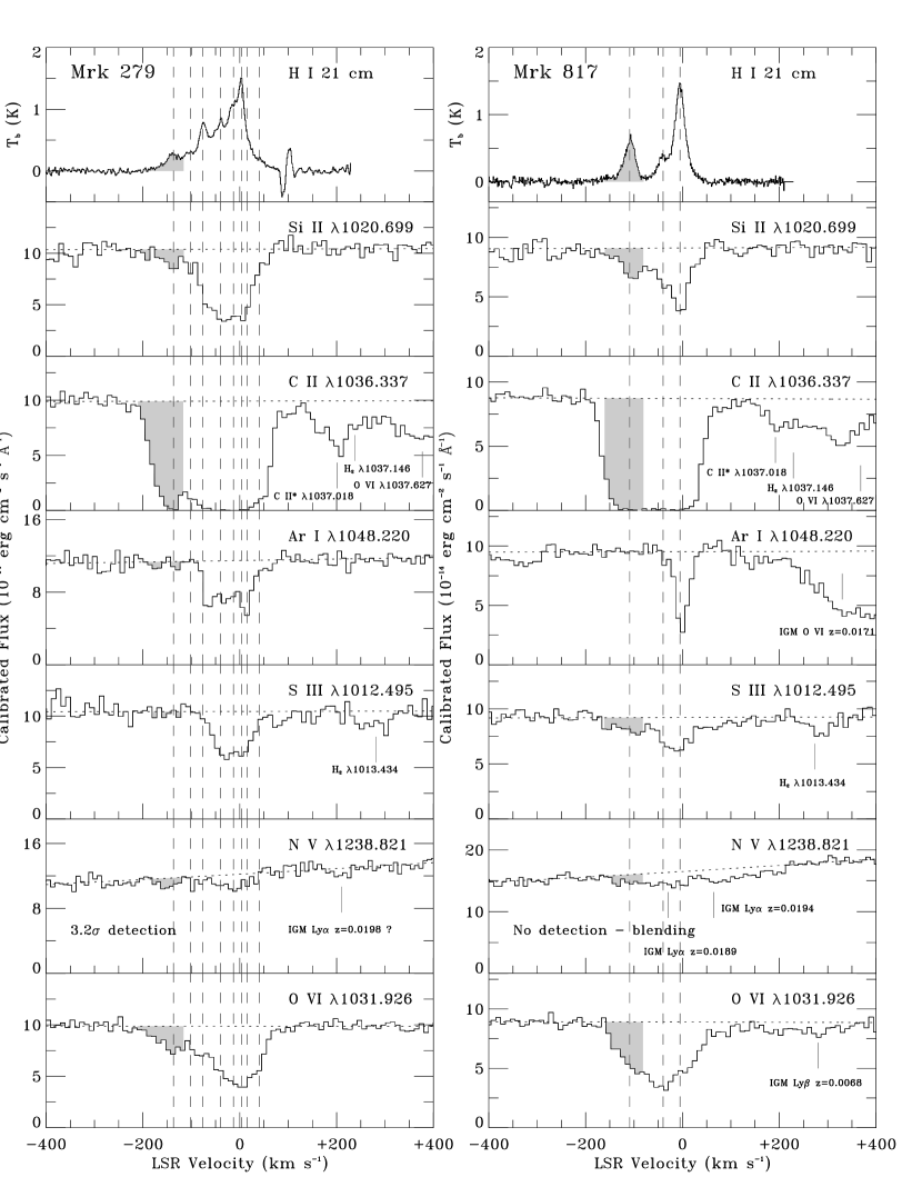
Figure 2: FUSE absorption line profiles of Si II, C II, Ar I, S III, and O VI, GHRS N V data, and Effelsberg 100m radio telescope H I 21 cm emission line observations (Wakker et al., 2001) toward Mrk 279 and Mrk 817. Gray shading is used to denote absorption (or emission) in the velocity range of Complex C. Dashed lines indicate the peaks of the neutral hydrogen emission, and dotted lines indicate the position of our fitted continuum in each absorption line. Other absorption lines falling in the range $-400<v_{LSR}<400$ km s^-1 of each line are identified with annotated tick marks. High-velocity highly ionized gas is detected in O VI along each sight line, and marginally detected in N V (3.2$\sigma$) toward Mrk 279. What appears to be high-velocity N V toward Mrk 817 is in fact a blend with intergalactic Ly$\alpha$ at $z=0.0189$.

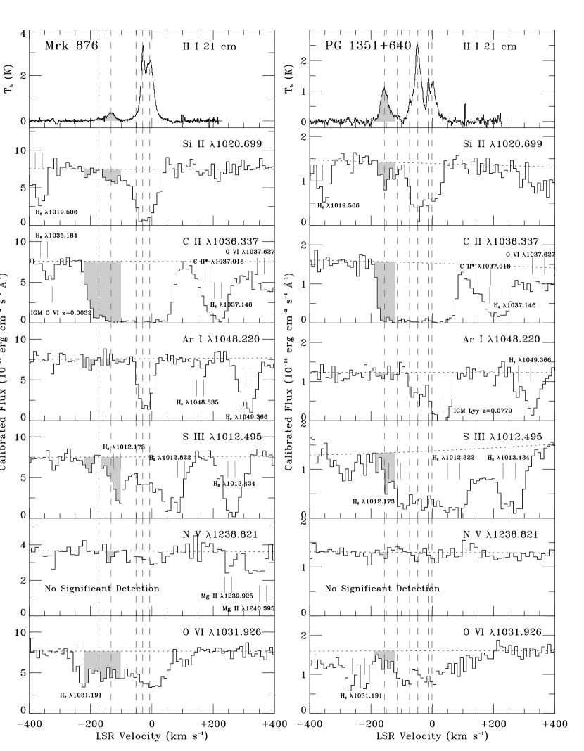
Figure 3: FUSE absorption line profiles of Si II, C II, Ar I, S III, and O VI, STIS N V data, and Effelsberg 100m radio telescope H I 21 cm emission line data (Wakker et al., 2001) toward Mrk 876 and PG 1351+640. Galactic blends have a two-component structure in these directions. High-velocity highly ionized gas is detected in O VI along each sight line, but not in N V.

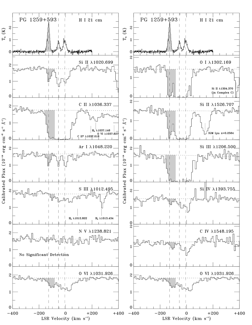
Figure 4: FUSE, STIS, and Effelsberg 100m radio telescope observations of the PG 1259+593 sight line. The H I and O VI profiles have intentionally been included in both columns for comparison. Highly ionized (Si IV, C IV, and O VI) and intermediate ionization (S III and Si III) gas is detected at Complex C velocities ($-160<v_{LSR}<-80$ km s^-1).

Figures 2, 3, and 4 display stacks of absorption line and H I 21 cm emission line profiles for Mrk 279 and Mrk 817, Mrk 876 and PG 1351+640, and PG 1259+593 respectively. Dashed vertical lines correspond to the peaks in the neutral hydrogen emission line profile given in the top panel, and show the velocities at which the neutral gas column density is highest. Dotted lines illustrate our continuum placement, chosen using the technique described in §3. Absorption in the velocity range corresponding to Complex C absorption is shaded in gray, according to the limits quoted in Table 4 – we note that the width of the Complex C absorption components may vary between species, hence the shading is included principally for illustrative purposes. Short vertical tick marks indicate the location of absorption blends. For Galactic blends, the tick marks designate the velocity where we expect the component to appear, assuming the absorbing ion occurs at the same velocity as the neutral hydrogen. In the cases of Mrk 876 and PG 1351+640, many of the blends have a two-component structure, which is marked accordingly. For extragalactic blends, where the absorption blend occurs at higher redshift, the tick marks simply designate the line center of the blend.

5.1 Mrk 279

The H I profile towards Mrk 279 shows eight components between $-150$ and 50 km s^-1, including two Complex C features at $-137$ and $-102$  km s^-1 (left panel of Figure 2). There appears to be corresponding absorption centered near $-137$ km s^-1 in the Si II, C II, N V and O VI profiles. The detection of high-velocity N V absorption, although tentative, is particularly interesting, and was first reported in Penton, Stocke, & Shull (2000). This feature is centered at $-149\pm 5$ km s^-1, and we measure its equivalent width as $17\pm 5\pm 3$ mÅ, between the velocity limits of $-190$ and $-115$ km s^-1, corresponding to log $N$(N V)$=12.93^{+0.12~{}+0.02}_{-0.17~{}-0.01}$. Since the systematic errors change the equivalent width but not the presence of the feature (i.e., it could be $14\pm 5$ or $20\pm 5$ mÅ), the formal significance of the high-velocity N V detection is $17/5>3\sigma$. This absorption extends down to $-190$ km s^-1, not to $-210$ km s^-1 as do the other ions shown in Figure 2. The large number of neutral hydrogen components present in this direction makes the separation of low and high-velocity gas difficult. However, it is striking how the high-velocity O VI absorption traces the shape of the C II absorption closely; on the negative side of the high-velocity absorption, both ions recover to the continuum just beyond $-210$ km s^-1, and on the positive side they both start to recover at $-115$ km s^-1. Though the C II line is heavily saturated, damping wings would not appear unless $N$(C II) $\gtrsim 10^{21}$ cm^-2, so the observed wings are likely kinematic, not Lorentzian. With our chosen velocity limits, we measure $W_{\lambda}$(O VI)$=53\pm 6\pm 7$ mÅ, corresponding to log $N$(O VI)$=13.66^{+0.04~{}+0.05}_{-0.04~{}-0.04}$. Gaussian component fitting reveals the center of this absorption to be $-133\pm 6$ km s^-1, which (within the error) is the same velocity as the H I line center ($-137$ km s^-1).

5.2 Mrk 817

Complex C gas is very pronounced in the H I profile towards Mrk 817, with a strong, distinct component centered at $-109$ km s^-1 (right panel of Figure 2). This feature is mirrored in the Si II, C II, S III, and O VI profiles, which all display clear absorption at this velocity. The S III detection is the strongest among all the Complex C sight lines, with an equivalent width $W_{\lambda}$(S III)$=32\pm 3\pm 10$ mÅ, and a central velocity of $-114\pm 9$ km s^-1, showing a kinematic connection between the neutral and intermediate-ionization gas. We do not expect contamination from the H₂ (0–0) P(2) $\lambda 1012.173$ line, since there is no H₂ absorption out of the $J=2$ levels in this direction. A double intergalactic Ly$\alpha$ feature happens to occur at just the redshift to blend with N V $\lambda 1238.821$, so although at first glance N V absorption appears to be present, we have no way of knowing conclusively. Strong broadening from the IVC at $-40$ km s^-1 blends with high-velocity O VI absorption, so the true extent of high-velocity O VI is hard to ascertain, but with a velocity range choice of $-160$ to $-80$ km s^-1 we obtain $W_{\lambda}$(O VI)$=93\pm 2\pm 29$ mÅ, and hence log $N$(O VI)$=13.97^{+0.02~{}+0.08}_{-0.02~{}-0.11}$. The mean O VI velocity is $-109\pm 10$ km s^-1, exactly the same as the H I centroid. What appears to be a positive velocity wing in the O VI profile is actually an intergalactic Ly$\beta$ absorber at $2360\pm 330$ km s^-1, a velocity which suggests an association with the Canes Venatici galaxy grouping (Tully, 1988).

5.3 Mrk 876

The Mrk 876 sight line (left panel of Figure 3) has a two-component high-velocity H I profile, with a very weak $-173$ km s^-1 component and a stronger $-133$ km s^-1 component, seen weakly in Si II and more clearly in O VI. The Ar I and N V lines show no significant high-velocity detection. C II $\lambda 1036.337$ is too saturated to make measurements near the line center, but reveals the presence of absorption out to $-220$ km s^-1. High-velocity S III absorption is hard to separate from the strong molecular hydrogen absorption in this direction. The high-velocity O VI absorption is extended and broad, with no recovery to the continuum out to $<-220$ km s^-1, at which velocity a blend with H₂ (6–0) P(3) $\lambda 1031.191$ becomes significant. We measure the velocity centroid of O VI to be $-148\pm 9$ km s^-1, which is only different from that of the H I component at the 2$\sigma$ level; given the strong blending from H₂ lines, we cannot say whether this difference is real. With log $N$(O VI)$=14.12^{+0.02~{}+0.09}_{-0.02~{}-0.11}$, Mrk 876 has the highest high-velocity column density of O VI of any Complex C sight line in our sample, yet with log $N$(H I)$=19.39\pm 0.02$ the lowest neutral hydrogen column density.

5.4 PG 1351+640

The PG 1351+640 sight line has strong high-velocity H I emission at $-158$ km s^-1, and a weaker component at $-115$ km s^-1 (right panel of Figure 3). Absorption at this velocity is not clear in Ar I, but clearly exists in Si II and C II. No high-velocity gas is apparent in S III; the high column density of molecular hydrogen along this sight line causes strong blending between H₂ P(4) (8–0) $\lambda 1012.261$ and the S III line and makes an assesment of the presence of high-velocity S III absorption difficult. Note that the molecular hydrogen lines in our plots have a two-component nature, due to local and IVC absorption. Absorption is present in O VI, but its extent is hard to ascertain, because of broad local absorption near 0 km s^-1, and blending with H₂ (6–0) P(3) $\lambda 1031.191$ below $-200$ km s^-1. Integrating over the optical depth profile reveals an O VI central velocity of $-147\pm 10$ km s^-1, 11 km s^-1 redward of the H I. We measure an upper limit of log $N$(N V)$<13.39$ and log $N$(O VI)$=13.66^{+0.08~{}+0.11}_{-0.08~{}-0.15}$, among the lowest columns of high-velocity O VI in our five sight lines, 0.46 dex less than the value towards Mrk 876. We also note the presence of an extended positive velocity wing in O VI, the like of which has been noted by S03 in 22 sight lines, 18 of which lie in the Northern Galactic hemisphere. Although apparently unrelated to Complex C gas, these wings nonetheless constitute a tracer of highly ionized high-velocity gas whose origin is unknown.

5.5 PG 1259+593

Two stacks of absorption lines for PG 1259+593 are presented in Figure 4, since in this case we have the benefit of STIS E140M data with extensive wavelength coverage. We include the H I and O VI profiles in both panels for ease of comparison. The structure of the nearby absorption along the PG 1259+593 sightline is clearly illustrated in the H I profile, which shows three distinct components: zero-velocity absorption, presumably tracing nearby gas, intermediate-velocity gas (centered at $v=-54$ km s^-1) and high-velocity gas (centered at $v=-128$ km s^-1). These components are clearly mirrored in absorption in Si II $\lambda 1020.699$ and Ar I $\lambda 1048.220$, and trace the densest regions of gas along the sight line. An extra absorption component along this sight line at $v=-110$ km s^-1 was suggested by Richter et al. (2001a), upon detailed analysis of STIS data, and has been confirmed by component fitting of the O I $\lambda 1302.169$ line (Sembach et al., 2003b). S III is detected in Complex C with an equivalent width $W_{\lambda}$(S III)$=17\pm 5\pm 12$ mÅ.

With regard to the highly ionized Complex C gas, components of absorption are clearly seen at Complex C velocities in Si IV, C IV and O VI. In each of these three cases, the weaker member of the resonance doublet was of no value in measuring a column density, due to either a lack of discernable absorption, or contamination from other lines. We measure log $N$(Si IV)$=12.73^{+0.02~{}+0.03}_{-0.01~{}-0.02}$, log $N$(C IV)$=13.26^{+0.03~{}+0.01}_{-0.04~{}-0.02}$, and log $N$(O VI)$=13.71^{+0.04~{}+0.05}_{-0.04~{}-0.05}$. High-velocity N V absorption is not seen in the data; we measure a $3\sigma$ upper limit to the high-velocity N V column density of log $N$(N V)$<12.85$. This non-detection is qualitatively consistent with the low N/O ratio measured by Richter et al. (2001a) and Collins et al. (2003a) in this direction. The kinematics of the high-velocity absorption are interesting, since we measure $\bar{v}$(Si IV)$=-119\pm 3$ km s^-1, $\bar{v}$(C IV)$=-106\pm 4$ km s^-1, and $\bar{v}$(O VI)$=-110\pm 5$ km s^-1, all by component fitting. This sight line thus exhibits a $18\pm 6$ km s^-1 difference between the centers of velocity of H I and O VI, with the C IV appearing to follow the O VI, and the Si IV falling inbetween. The intermediate-ionization S III line has a velocity centroid of $-104\pm 9$ km s^-1. Note that absorption from Si II, Si III, and Si IV is seen over the same velocity range.

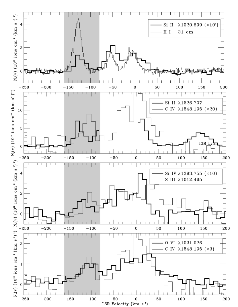
Figure 5: Plots of apparent column density as a function of velocity, for various absorption lines and H I emission toward PG 1259+593. In each panel, one of the profiles has been scaled for ease of comparison to the other species. The velocity range corresponding to Complex C absorption is shaded in gray. Note that in the second panel, we have not included Si II $\lambda 1526.707$ absorption between $v=-75$ and 0 km s^-1, since the line is heavily saturated in this region. The two-component high-velocity structure is most easily seen in this second panel.

To further illustrate the kinematic structure of the Complex C gas toward PG 1259+593, we compare apparent column density profiles of various species in Figure 5. In each panel one of the profiles has been normalized in order to compare its shape with the other profile. We include ions that trace low-ionization gas (H I and Si II), intermediate ionization gas (S III), and highly ionized gas (Si IV, C IV, and O VI). Complex C absorption is clearly seen in all these ionic species. The two component high-velocity structure is most easily seen in the second panel, where we compare Si II $\lambda 1526.707$ with C IV $\lambda 1548.195$ from the STIS data. We return to a discussion of the absorption kinematics in §8.2.

6 Potential Ionization Mechanisms

In studying highly ionized gas in HVCs our ultimate goal is to determine the ionization mechanism(s). Not only is this interesting in its own right, but also knowledge about ionization may be able to provide information on the location of HVCs. In this section we describe the potential mechanisms that could create highly ionized gas in or around HVCs.

6.1 Collisional Ionization Equilibrium (CIE)

Perhaps the simplest picture that can account for simultaneous observations of Si IV, C IV, and O VI (as seen toward PG 1259+593) is one involving a cloud of gas at a fixed kinetic temperature, with every collisional ionization balanced by a radiative recombination. Sutherland & Dopita (1993) calculated the fraction of each element in each ionization stage, assuming these equilibrium conditions. To test to see if CIE conditions exist, one needs to find that the column densities of multiple ions are simultaneously consistent with the model predictions at one temperature. However, in interstellar and intergalactic environments, such conditions rarely apply to the O VI ion, since it exists at temperatures of a few $\times 10^{5}$ K where the cooling function is maximized. When cooling occurs faster than recombination the ionization can become “frozen-in”, producing gas referred to as overionized (Kafatos, 1973). A single phase of hot gas under CIE conditions would be traced by absorption at the same central velocity in all ions. Velocity offsets cannot be explained by a single-phase, single-temperature CIE model.

6.2 Photoionization

The high ions Si IV, C IV, N V, and O VI require energies of 33.5, 47.9, 77.5, and 113.9 eV respectively for their creation. If the radiation field is hard enough to contain significant intensities of photons at these energies, the ions can be produced directly by photoionization. S03 have conducted photoionization models to investigate the ionization fraction of O VI ($f_{O~{}VI}$) in HVCs as a function of neutral hydrogen column density and ionization parameter $U=n_{\gamma}/n_{H}$, where $n_{\gamma}$ and $n_{H}$ are the photon density and total hydrogen density, respectively. The models assumed the gas is optically thin to ionizing and cooling radiation (i.e. log $N$(H I)$<17.2$), and took the QSO spectral energy distribution (SED) from Madau (1992), normalized at 912  Å to $J_{{\nu}_{0}}=1\times 10^{-23}$ erg cm^-2 s^-1 Hz^-1 sr^-1 (Haardt & Madau, 1996). The S03 photoionization models provides a strong conclusion: to produce an O VI column density of 10¹⁴ cm^-2 requires the HVC to be several hundred kiloparsecs in depth, for any metallicity in the range $Z=0.01$–$1.0Z_{\odot}$. These sizes are far too large to be consistent with most models of HVCs; Blitz et al. (1999) predict typical diameters of $\sim 25$ kpc; theories that place HVCs closer to the Milky Way predict even smaller sizes. If the H I column density in the model is increased above log $N$(H I)$<17.2$, so that the cloud is no longer optically thin, the predicted O VI and C IV column densities drop, and the conclusion becomes even stronger: O VI is most likely collisionally ionized.

More detailed photoionization modeling of the high ions in Complex C would need to include the effect of ionizing photons escaping from the Galactic disk. A key uncertainty in doing this is the escape fraction of ionizing photons (Bland-Hawthorn & Maloney, 1999). The strong He II ionization edge at 54 eV in hot star spectra limits the flux of photons energetic enough to produce either N V or O VI. Therefore, in studies of highly ionized gas in the ISM of the Milky Way, N V and O VI are almost always interpreted as being tracers of collisionally ionized gas (e.g. Savage et al., 2003; Fox et al., 2003). So, modifications to the radiation field will be more significant for calculating the ion fractions of low and intermediate ionization species, than for high ions such as O VI.

6.3 Radiatively Cooling Gas Flows (RC)

As hot ($T_{0}\gtrsim 10^{6}$ K) gas cools down by radiative recombination it will pass through the temperature regime at which high ions such as N V and O VI exist. Edgar & Chevalier (1986) estimated the ionization properties of a body of gas cooling from an initial high temperature ($T=10^{6}$ K), for a variety of cases ranging from isochoric (constant density) to isobaric (constant pressure). Their models predict the column density of Si IV, C IV, N V, and O VI; for the case of O VI, the column density is given by $N$(O VI) $=4-6\times 10^{14}(v_{cool}/10^{2}$ km s^-1) cm^-2, assuming solar abundances, where $v_{cool}$ is the flow velocity. Heckman et al. (2002), upon discovering a correlation between line width and column density in O VI absorbers across a wide variety of locations, have suggested that all O VI absorbers can be explained by radiatively cooling hot gas passing through transition temperatures. This conclusion remains the same over a wide range of metallicity. This result relies on there being a linear relationship between the characteristic flow velocity and the non-thermal line broadening parameter $b_{nt}$.

If the RC model is to give a complete description of the highly ionized gas present in or near HVCs, it would need to account for the origin of the hot gas in the first place, and the kinematical alignments between neutral and ionized phases of gas that are reported in this paper.

6.4 Conductive Interfaces (CI)

When reservoirs of hot and cold gas come into contact with one another, electron collisions will conduct energy from the hot medium towards the cooler medium, at a rate depending on the plasma conductivity and the orientation of the magnetic field relative to the interface. Transition-temperature ions, such as C IV, N V, and O VI, can be produced in the conduction front as the cooler gas evaporates and the hotter gas condenses.

Borkowski, Balbus, & Fristrom (1990) studied the energy transport when a planar front is established between an interstellar cloud and a hot ($T\sim 10^{6}$ K) coronal medium. The calculations of Borkowski et al. (1990) predict the expected column densities of the ions Si IV, C IV, N V, and O VI produced in a conductive interface, as a function of both time and the angle $\theta$ between the normal to the front and the magnetic field. We consider magnetic field orientations of $\theta=0\arcdeg-85\arcdeg$ and interface ages of log [$t$(yr)] $=5.0-7.0$. Since the thermal conductivity of plasma is far greater along magnetic field lines than across them, the conduction is quenched when the field runs parallel to the interface, and so the predicted high ion column densities are much lower in this case. As with any interface model, the CI theory predicts that there should be no (or small) velocity offsets between high ions observed at the surface of the cloud and neutral ions observed within it. Furthermore, the line widths are predicted to be thermally dominated. These conditions provide a set of diagnostic tests that can be applied when trying to explain the origin of an O VI absorber.

6.5 Turbulent Mixing Layers (TML)

Turbulence is increasingly being considered to be a ubiquitous phenomenon in the ISM. In an interface between turbulent hot gas and a region of cold gas, any relative motion of the gas phases can generate Kelvin-Helmholtz instabilities that mix the hot and cold gases together in a mixing layer. Such a layer would be at transition temperatures, sufficiently hot to generate ions such as N V and O VI by electron collisions. TML theory was introduced by Begelman & Fabian (1990), who argued that conduction will only form a significant mechanism of energy transport in a quiescent medium, but in the turbulent hot ISM tangled magnetic fields will suppress conduction. Slavin, Shull & Begelman (1993) developed the TML theory to predict high ion column densities, as a function of the entrainment velocity and mixing-layer temperature.

We consider the TML predictions with the entrainment velocity of the gas flow in the range $25-100$ km s^-1, and the temperature of the post-mixed gas in the range log $T=5.0-5.5$. A key difference between TML theory and other ionization models is a high $N$(C IV)/$N$(O VI) ratio; observation of this quantity thus provides a key test of the TML theory.

6.6 Shock Ionization (SI)

If a high-velocity cloud passes through a surrounding medium at a velocity higher than the local sound speed, a shock front will develop at the leading edge of the cloud. The temperature in the gas behind the front could then be raised to levels at which highly ionized material can be formed by collisional ionization ($T\gtrsim 10^{5}$ K). Dopita & Sutherland (1996) generated a grid of low-density shock models, predicting the column density of high ions for shock velocities in the range $150<v_{S}<500$ km s^-1, assuming solar abundances. In this study we consider the SI model with shock velocities of $150-500$ km s^-1 and magnetic parameters $0\leq B_{0}/n_{0}^{3/2}\leq 4\,\mu\mathrm{G\,cm}^{-3/2}$.

In the shock ionization model, the shock velocity is the key parameter determining the expected column densities of high ions. We note that since Complex C is falling toward the Galaxy (at $\approx 130$ km s^-1), any Galactic wind or fountain outflow would serve to increase the Mach number and hence the strength of the shock. In this scenario, the interaction of the cloud with the surrounding environment would be contributing to both the ionization and the metallicity of the cloud gas. Instabilities arising from the interaction of a HVC with magnetic fields could also influence the ionization properties of the cloud (Konz et al., 2001).

6.7 Supernova Remnants (SNR)

Slavin & Cox (1992) and Shelton (1998) have considered the evolution of low density supernova remnants expanding into a surrounding medium. However, since no stars have ever been detected in HVCs despite extensive searches (Hopp, Schulte-Ladbeck, & Kerp, 2003; Willman et al., 2002; Davies et al., 2002), we do not expect them to harbor SNRs, and so we do not consider the SNR model any further.

7 Non-Solar Abundance Issues

A difficulty we face in applying ionization models to Complex C is the fact that the elemental abundance ratios are known to be non-solar in the complex. In this section we investigate the effect that changed abundances will have on the model high ion column density predictions.

In any model where the predicted columns of high ions are regulated by radiative cooling losses, the O VI column densities are fairly insensitive to metallicity. This is because oxygen is the primary coolant for interstellar gas with log $T=5.0-5.6$, and so reducing the oxygen abundance reduces the cooling rate, and hence lengthens the cooling time of the gas. This feedback effect causes the predicted columns to be fairly constant over metallicity (Edgar & Chevalier, 1986; Heckman et al., 2002). Savage et al. (2003) discuss how the expected value of $N$(O VI) depends on the metallicity in the cooling gas of a Galactic fountain flow. Since the total column density of cooling gas is given by $N_{cool}=\dot{N}_{\mathrm{H}}t_{cool}$, where $\dot{N}_{\mathrm{H}}$ is the flux of cooling gas (hydrogen ions cm^-2 s^-1) and $t_{cool}$ is the cooling time of the gas, the expected column density of O VI is given by

$$N(\mathrm{O~{}VI})=f_{\mathrm{O~{}VI}}A_{\mathrm{O}}\dot{N}_{\mathrm{H}}t_{cool},$$ (6)

where $f_{\mathrm{O~{}VI}}$ is the fraction of oxygen atoms present as O VI, and $A_{\mathrm{O}}$ is the abundance of oxygen with respect to hydrogen.

It is often assumed for departures from solar abundances that $t_{cool}\,{\propto}\,n_{\mathrm{H}}^{-1}A_{Z}^{-1}$, where $n_{\mathrm{H}}$ is the initial ionized hydrogen density in the cooling gas and $A_{Z}$ is the mean metallicity of the dominant coolants in the gas. This relation assumes that the cooling is dominated by the radiative emission produced by the heavy elements. Since oxygen is the most important coolant, we take $A_{Z}=A_{\mathrm{O}}$, and therefore $N$(O VI)$\,\propto f_{\mathrm{O~{}VI}}\dot{N}_{\mathrm{H}}n_{\mathrm{H}}^{-1}$, which is independent of the oxygen abundance. Since $\dot{N}_{\mathrm{H}}n_{\mathrm{H}}^{-1}$ has dimensions of velocity, we can identify $\dot{N}n_{\mathrm{H}}^{-1}\equiv v_{cool}$, so that $N$(O VI)$\,\propto f_{\mathrm{O~{}VI}}v_{cool}$.

However, the calculations of Benjamin, Benson, & Cox (2001) show that the cooling time scales more like $t_{cool}\,{\propto}\,n_{\mathrm{H}}^{-1}A_{Z}^{-\beta}$, where $\beta\approx 0.85$ over the range $Z=0.1-1.0Z_{\odot}$. Physically, this effect is due to the inclusion of cooling from hydrogen and helium as well as metal line cooling. In this case, the expected column density of O VI will scale as

$$N(\mathrm{O~{}VI})\,\propto A_{\mathrm{O}}^{1-\beta}v_{cool}$$ (7)

So, if the abundance of oxygen changes from $A_{\mathrm{O}}^{\odot}$ to $A_{\mathrm{O}}^{\prime}$, then the predicted column density of O VI will change from $N$(O VI)^⊙ to $N$(O VI)^′ according to

$$\frac{N(\mathrm{O~{}VI})^{\prime}}{N(\mathrm{O~{}VI})^{\odot}}=\left(\frac{A_{\mathrm{O}}^{\prime}}{A_{\mathrm{O}}^{\odot}}\right)^{1-\beta}.$$ (8)

For elements other than oxygen, which are less important coolants, the predicted column densities will also scale as $N(\mathrm{X})^{\prime}/N(\mathrm{X})^{\odot}=(A_{\mathrm{O}}^{\prime}/A_{\mathrm{O}}^{\odot})^{1-\beta}$, provided that $A_{\mathrm{X}}^{\prime}/A_{\mathrm{X}}^{\odot}=A_{\mathrm{O}}^{\prime}/A_{\mathrm{O}}^{\odot}$. However, if there are deviations from the solar ratios among the other heavy elements, then

$$\frac{N(\mathrm{X})^{\prime}~{}}{N(\mathrm{X})^{\odot}}=\frac{(A_{\mathrm{X}}/A_{\mathrm{O}})^{\prime}~{}(A_{\mathrm{O}}^{\prime})^{1-\beta}}{(A_{\mathrm{X}}/A_{\mathrm{O}})^{\odot}(A_{\mathrm{O}}^{\odot})^{1-\beta}}=\frac{A_{\mathrm{X}}^{\prime}}{A_{\mathrm{X}}^{\odot}}\left(\frac{A_{\mathrm{O}}^{\prime}}{A_{\mathrm{O}}^{\odot}}\right)^{-\beta},$$ (9)

where X could represent either Si IV, C IV, or N V. Combining equations (8) and (9) leads to the shift applied to the logarithmic column density ratios

$$\mathrm{log}\left[\frac{N(\mathrm{X})}{N(\mathrm{O~{}VI})}\right]^{\prime}\!=\mathrm{log}\left[\frac{N(\mathrm{X})}{N(\mathrm{O~{}VI})}\right]^{\odot}\!+\Delta(\mathrm{log}~{}A_{\mathrm{X}})-\Delta(\mathrm{log}A_{\mathrm{O}}),$$ (10)

where $\Delta(\mathrm{log}\,A_{\mathrm{X}})=\mathrm{log}\,A_{\mathrm{X}}^{\prime}-\mathrm{log}\,A_{\mathrm{X}}^{\odot}=\mathrm{log}(A_{\mathrm{X}}^{\prime}/A_{\mathrm{X}}^{\odot})$ is the change in the logarithmic abundance of element X. It can be seen from Equation 10 that the adjusted logarithmic column density ratios are independent of the exact value of $\beta$.

These arguments were originally formulated for the case of pure radiatively cooling gas flows (see §6.3), but equally apply to all other models considered in §6.3–§6.6, since the rate of cooling is a critical component of all the other models. It should be emphasized that these results are approximate and neglect the contribution to the cooling by other elements (particularly carbon and nitrogen). Nonetheless, this is a first attempt at quantifying the effects of low metallicities on high ion production. Equation 10 has to be applied twice in order to apply the model ionic ratio predictions to the Complex C gas; these two corrections are described in the next two subsections.

The one model where cooling is not important is the CIE model (§6.1), since in this scenario the temperature is held fixed, and the equilibrium ionization balance calculated. In this case, the expected column density of a given ion is proportional to the fraction of the element in the relevant ionization stage (tabulated in Sutherland & Dopita, 1993), multiplied by the abundance of the element.

7.1 Updates to Solar Abundance Ratios

The models described in §6 each assumed different solar elemental abundance ratios, according to the most up-to-date abundances that were available when the models were published. However, the solar abundances have recently undergone several important revisions, as can be seen in Table 5, in which we summarize all significant published values for the solar composition. We made a correction so that each ionization model is adjusted to the same set of solar abundances. We decided to take the solar oxygen abundance (log $A_{\mathrm{O}}^{\odot}=-3.31$) from Allende Prieto, Lambert, & Asplund (2001), the solar carbon abundance (log $A_{\mathrm{C}}^{\odot}=-3.61$) from Allende Prieto, Lambert, & Asplund (2002), and the solar nitrogen and silicon abundances (log $A_{\mathrm{N}}^{\odot}=-4.07$; log $A_{\mathrm{Si}}^{\odot}=-4.46$) from Holweger (2001). These abundances are significantly different (up to 0.2 dex) from the widely used tables of Anders & Grevesse (1989). By finding the difference $\Delta A_{\mathrm{X}}$ between the solar abundances used in each model calculation and our adopted solar abundances, we brought all model predictions onto a unified solar abundance scheme, using equation (10) in the form

$$\mathrm{log}\left[\frac{N(\mathrm{X})}{N(\mathrm{O~{}VI})}\right]^{\odot}_{new}\!\!\!\!=\mathrm{log}\left[\frac{N(\mathrm{X})}{N(\mathrm{O~{}VI})}\right]^{\odot}_{old}\!\!\!\!+\Delta(\mathrm{log}\,A_{\mathrm{X}}^{\odot})-\Delta(\mathrm{log}\,A_{\mathrm{O}}^{\odot}).$$ (11)

where the shifts $\Delta(\mathrm{log}\,A_{\mathrm{X}}^{\odot})$ are in the sense “new minus old”.

7.2 Corrections for Environments with Non-Solar Abundance Ratios

The second correction we make is to account for the fact that relative abundance ratios in Complex C are known to be non-solar (Wakker et al., 1999; Richter et al., 2001a; Gibson et al., 2001; Collins et al., 2003a; Tripp et al., 2003; Sembach et al., 2003b). Caution is necessary when interpreting various measurements of [X/H], since this number depends upon the assumed solar elemental abundances. In Table 6 we have taken all recent measurements of the metallicity of Complex C and adjusted them to our adopted abundances presented in Table 5. It can be seen that all measurements of [O/H] in Complex C converge to a 0.41 dex region between $-0.86$ to $-0.45$; toward PG 1259+593 the updated measurements all lie between $-0.86$ and $-0.79$. Given the errors there is no strong evidence for any variation in these abundances. The O I/H I ratio is a sensitive measure of the overall metallicity of the system, for a number of reasons. The depletion of oxygen onto dust is small (e.g. Moos et al., 2002), ionization effects are minimal since the ionization potentials of O I and H I are very similar, and charge-exchange reactions couple the elements together (Field & Steigman, 1971). The latter two effects ensure that the ionization fractions of O and H track each other very closely. We now wish to determine the best estimates of [X/H] in Complex C for each of the elements oxygen, nitrogen, silicon, and carbon so as to adjust the model predictions accordingly. For this purpose we use the Sembach et al. (2003b) measurement of $N$(H I) $=19.94\pm 0.06$ in the main component of Complex C toward PG 1259+593.

For oxygen, we use the most recent determination along the PG 1259+593 sight line of [O/H]${}_{C}=-0.79$ from Sembach et al. (2003b), who used the same set of solar abundances as our adopted values.

For nitrogen we use log $N$(N I) $=14.02$ in the Complex C gas toward PG 1259+593 (Collins et al., 2003a). We also measure the high-velocity N II $\lambda 1083.994$ towards PG 1259+593 to have an equivalent width of $111\pm 4\pm 25$ mÅ between $-160$ and $-80$ km s^-1, which using the AOD technique corresponds to log $N$(N II) $=14.24\pm 0.02\pm 0.14$. We have no way of measuring $N$(H II) in Complex C, which would allow us to explicitly calculate [N/H] = [N I+N II]/[H I+H II]. However, we use the results of Collins et al. (2003a), who used photoionization modelling to find that the ionization correction for nitrogen is negligible, so that [N I/H I] $\approx$ [N/H]. This result implies that essentially the N I and H I reside together in the neutral gas, and the N II and H II reside together in the ionized gas, as might be expected since the first ionization potentials of hydrogen and nitrogen are so close. Combining the $N$(N I) measurement with $N$(H I) leads to [N/H]${}_{C}=-1.85$.

For silicon, we utilize the (Collins et al., 2003a) measurement of log $N$(Si II) $=14.67$ toward PG 1259+593, so that [Si II/H I] $=-0.81$. These authors found that the Si ionization correction [Si II/H I] $-$ [Si/H] $\approx 0.2$ dex for log $N$(H I) $=19.94$. With this assumption we derive [Si/H]${}_{C}=-1.01$.

Unfortunately, for the Complex C gas, no unsaturated absorption lines of carbon are available in either the FUSE or HST bandpass, from which we could make a carbon abundance measurement, and the intersystem C II transition at 2325Å is too weak to measure. So, we decided to estimate the relative carbon abundance in Complex C by examining the behavior of C/O versus metallicity as reported in the literature. In general, C/O is known to be an increasing function of O/H at high metallicity, but is much flatter at low metallicity (Henry, Edmunds, & Köppen, 2000; Garnett et al., 1995). The C/O ratio appears to plateau at log (C/O) $\approx-0.65\pm 0.1$ in the Henry et al. (2000) data for low metallicity (log $A_{\mathrm{O}}<-4$) extragalactic H II regions and stars, and although Complex C could have a different nucleosynthetic history, we assume this ratio applies there. Combining this estimate with the other abundance measurements discussed above we adopt

$$\mathrm{(C/O)}_{C}= 0.45\mathrm{(C/O)}_{\odot}\;\; \Rightarrow\mathrm{[C/O]}_{C}=-0.35$$

$$\mathrm{(N/O)}_{C}= 0.09\mathrm{(N/O)}_{\odot}\;\; \Rightarrow\mathrm{[N/O]}_{C}=-1.06$$ (12)

$$\mathrm{(Si/O)}_{C}= 0.60\mathrm{(Si/O)}_{\odot}\;\; \Rightarrow\mathrm{[Si/O]}_{C}=-0.22.$$

Finally, since $\Delta(\mathrm{log}\,{A_{\mathrm{X}}})=$ [X/H] and $\Delta(\mathrm{log}\,A_{\mathrm{O}})=$ [O/H], we can combine these abundances with equation (10) to generate the relation used to correct the solar model column density predictions to apply in Complex C.

$$\mathrm{log}\,\left[\frac{N(\mathrm{X})}{N(\mathrm{O~{}VI})}\right]_{C} = \mathrm{log}\,\left[\frac{N(\mathrm{X})}{N(\mathrm{O~{}VI})}\right]^{\odot}_{new}\!\!+[\mathrm{X}/\mathrm{H}]_{C}-[\mathrm{O}/\mathrm{H}]_{C}$$ (13)

$$= \mathrm{log}\,\left[\frac{N(\mathrm{X})}{N(\mathrm{O~{}VI})}\right]^{\odot}_{new}+[\mathrm{X}/\mathrm{O}]_{C}$$

Equations (11) and (13) were used to generate the modified ratio predictions contained in Table 7, for each of the models described in §6.3–6.6.

All model predictions discussed here have taken no account of elemental depletion into dust, which would further complicate the interpretation of the ionic ratios. However, Collins et al. (2003a) report solar [S/O] and [Si/O] ratios in Complex C, suggesting that dust depletion is not significant. This conclusion is reinforced by strong detections of Fe II in Complex C (Murphy et al., 2000; Tripp et al., 2003), who found that the measured iron abundances leave little room for depletion into dust. The absence of H₂ in Complex C (Richter et al., 2001b) is consistent with the absence of dust since H₂ is thought to form on the surface of dust grains.

Finally, note that (with the exception of carbon) we have used measured abundance ratios of the neutral gas in Complex C; if this HVC is interacting with a surrounding medium, then this medium could also display non-solar abundance patterns. In any model where gas is mixed between two media, non-solar abundance variations in the hot medium become a further complication, which is not accounted for here.

8 Comparison of Observations and Theory

8.1 Ionic Ratios

We focus our discussion of ionization on the high ions Si IV, C IV, N V, and O VI. The lower ion stages are more likely to be produced by photoionization, since there are many more ionizing photons below 50 eV capable of producing them. This origin has been suggested as an explanation for low ionization species in other high-velocity absorbers (e.g. Collins et al., 2003b, toward PKS 2155-304 and Mrk 509).

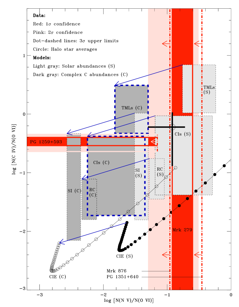
Figure 6: Plot of $N$(C IV)/$N$(O VI) against $N$(N V)/$N$(O VI) parameter space, comparing theory against observations. Our Mrk 279 and PG 1259+593 measurements are shown as colored regions, and the dot-dashed lines with arrows attached represent upper limits to the $N$(N V)/$N$(O VI) ratio for directions where no absolute $N$(N V) measurement could be made. The predictions of various models in two cases are shown: solar relative abundance ratios (light shaded regions), and assumed Complex C relative abundance ratios (dark shaded regions). The blue arrows connect the model predictions and show the size of the abundance correction we applied. Note that CIE = collisional ionization equilibrium, RC = radiative cooling , CI = conductive interfaces, TML = turbulent mixing layers, and SI = shock ionization. The model parameters are described in the text.

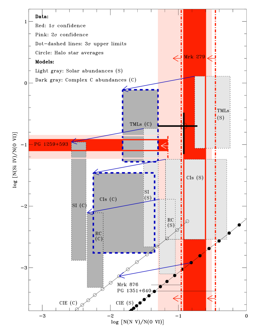
Figure 7: Same as Figure 6, except with $N$(Si IV)/$N$(O VI) as the ordinate.

The best data available exist for the PG 1259+593 sight line, for which we measure high-velocity ionic ratios of $N$(Si IV)/$N$(O VI) $=0.10\pm 0.02$, $N$(C IV)/$N$(O VI) $=0.35^{+0.05}_{-0.06}$, and $N$(N V)/$N$(O VI) $<0.07$ (3$\sigma$). Our other new results are measurements of the $N$(N V)/$N$(O VI) ratio: $0.19^{+0.06}_{-0.07}$ for Mrk 279, $<0.11$ for Mrk 876, and $<0.35$ for PG 1351+640. Our ionic ratio information is displayed graphically in Figures 6 and 7, which show log [$N$(C IV)/$N$(O VI)] versus log [$N$(N V)/$N$(O VI)], and log [$N$(Si IV)/$N$(O VI)] against log [$N$(N V)/$N$(O VI)] respectively. We choose to compare high ion column density ratios, rather than absolute column densities, to allow for multiple interfaces or regions along the line of sight where hot gas could exist. Using the model predictions summarized in Table 7, we can identify regions of this ionic ratio space that gas behaving according to the various models should occupy. Because of the various free parameters that can vary in each model, we assume the models to occupy boxes rather than lines in these ionic ratio diagrams. For each of four theories (CI, RC, TML, SI) we have computed the model predictions for the cases of solar abundances (light regions) and Complex C abundances (darker regions). The changes in the predicted ion ratios due to these abundance variations are fairly substantial. For ease of comparison, blue arrows connect the two boxes for each model.

It can be seen that the adjusted RC model significantly underestimates the observed $N$(C IV)/$N$(O VI), $N$(Si IV)/$N$(O VI), and $N$(N V)/$N$(O VI) ratios. The CIE model is incapable of simultaneously matching either the $N$(C IV)/$N$(O VI) or the $N$(Si IV)/$N$(O VI) ratio, in either abundance case. The SI model can successfully reproduce both the $N$(C IV)/$N$(O VI) or the $N$(Si IV)/$N$(O VI) ratios, but significantly underestimates the $N$(N V)/$N$(O VI) ratio toward Mrk 279 by over an order of magnitude. This narrows down the viable models to the CI and TML theories. The CI model can reproduce the $N$(C IV)/$N$(O VI) ratio toward PG 1259+593, but seems to underestimate the $N$(Si IV)/$N$(O VI) ratio along this sight line. The TML theory has the opposite problem: it can match the $N$(Si IV)/$N$(O VI) ratio but overestimates $N$(C IV)/$N$(O VI). Both these theories (when adjusted for Complex C abundances) predict $N$(N V)/$N$(O VI) ratios that are marginally lower than the value observed toward Mrk 279, but they do agree within the 2$\sigma$ error on the measurement. Note that although we have fully accounted for errors in the data, we have not fully accounted for errors in the model corrections. Uncertainties of $\sim 0.2$ dex are likely because of incomplete knowledge of the elemental abundances; perhaps a similar error arises from the assumption that the cooling is dominated by oxygen. From these two plots we conclude that TMLs or CIs could be potential explanations for the highly ionized material around Complex C. We have outlined these two model boxes in blue in Figures 6 and 7 to highlight their position.

Examining the CI model further, we note that the large size of the CI model box in the ionic ratio planes is largely due to the inclusion of interface age as a free parameter. As we have no way of knowing the age of an interface around Complex C, we chose to include a range from $10^{5}$ to $10^{7}$ years, a period which spans the transition from evaporative to condensing interfaces. The data are most consistent with young ($\sim 10^{5}$ yr) interfaces, since the adjusted-abundance CI boxes in Figures 6 and 7 overlap the data at their high $N$(X)/$N$(O VI) extents, which correspond to lower interface age. Physically this is because the O VI columns do not reach their maximum values until $\sim 10^{6}$ yr, but the other high ions peak in abundance at earlier interface age. The theory predicts $N$(O VI) $=10^{12}-10^{13}$ cm^-2 per interface (depending on the magnetic field direction), which we can correct by a factor of 0.8 to account for non-solar abundances. Even if we assume a magnetic field normal to the cloud boundary, we would still require between six to eighteen interfaces (i.e., three to nine clouds), to account for the observed O VI column densities in Complex C of $10^{13.66}-10^{14.12}$, with a larger number if the magnetic field has a component parallel to the boundary, quenching the conduction. In one particular case, we already know of a multiple component structure: two high-velocity neutral components are thought to exist toward PG 1259+593 (Richter et al., 2001a; Sembach et al., 2003b), providing four interfaces. Therefore, at least one more low density neutral absorber at Complex C velocities, with a pair of hot interfaces, is necessary to explain the O VI toward PG 1259+593 in the CI model. Such a component could be too close in velocity to the $-128$ km s^-1 component to be resolved with current instruments.

The $N$(Si IV) prediction may be the least robust of the various models, since Si IV has the lowest creation ionization potential (33.5 eV) of any of the high ions under study, and so is most susceptible to production by photoionization, for example by photons escaping the Galactic disk. This might lead to enhanced $N$(Si IV)/$N$(O VI) ratios over the individual model predictions, raising all boxes vertically upward toward the PG 1259+593 data point on Figure 7. Photoionization could also enhance the $N$(C IV)/$N$(O VI) ratio, if the radiation field were hard enough. On the other hand, depending on the slope of the ionizing spectrum, the $N$(Si IV)/$N$(O VI) ratio could also decrease if enough Si V is formed to depress the Si IV prediction. A more detailed understanding of the escaping radiation filed is needed to fully investigate the effect of additional photoionization. If it does play a role, then multiple ionization processes are occuring in HVCs, just as multiple ionization processes appear to be at work in the hot Galactic halo (Ito & Ikeuchi, 1988; Shull & Slavin, 1994; Savage et al., 2003; Zsargó et al., 2003).

8.2 Kinematic Information

Unfortunately, given the paucity of data points and the uncertainty in the model predictions stemming from the numerous metallicity issues, we cannot at this point uniquely specify the ionization mechanism purely from the ionic ratios. Analysis of ionic ratios has the further problem that multiple, separate regions of absorbing gas, closely related in velocity space, can contribute to the integrated column density along a line of sight, making interpretation of ionic ratios very difficult. However, the kinematics of the absorption provide further information; by comparing the extent and line centers of high-velocity absorption between species, one can gain useful information regarding the ionization mechanism.

In the case of Mrk 279 and Mrk 817, high-velocity absorption is detected in low and high ionization species at very similar velocities (Mrk 279: $\bar{v}_{\mathrm{O~{}VI}}=-133\pm 6$ km s^-1, $\bar{v}_{\mathrm{H~{}I}}=-137$ km s^-1; Mrk 817: $\bar{v}_{\mathrm{O~{}VI}}=-109\pm 10$ km s^-1, $\bar{v}_{\mathrm{H~{}I}}=-109$ km s^-1). In the other three sight lines the difference is less than 20 km s^-1. In Table 8 we list our measured central velocities of the high-velocity O VI, and compare them to both the centers of the H I and Si II components, and to earlier measures of the O VI velocities from S03. In our sample the average displacement $<\bar{v}_{\mathrm{O~{}VI}}-\bar{v}_{\mathrm{H~{}I}}>=3\pm 12$ km s^-1, where the error represents the standard deviation of the sample, whereas the S03 results (that used nine Complex C sight lines) have an average displacement $<\bar{v}_{\mathrm{O~{}VI}}-\bar{v}_{\mathrm{H~{}I}}>=0\pm 13$ km s^-1. The differences between our measurements and the S03 measurements of $\bar{v}_{\mathrm{O~{}VI}}$ are due to different data reduction pipelines (v2.1.6 versus v1.8.7), and in the case of PG 1351+640, our inclusion of new data. These changes caused the choice of velocity integration limits to change (when $v$ is measured using the moment of the optical depth technique), or by our using the component fitting method when the line center was more clearly defined. We also measure $<\bar{v}_{\mathrm{O~{}VI}}-\bar{v}_{\mathrm{Si~{}II}}>=0\pm 15$ km s^-1. These small differences between the velocities of O VI, Si II, and H I reveal a strong kinematic connection between the neutral and highly ionized gas in Complex C.

The observed velocity alignments are consistent with, and indeed suggestive of, an origin at some form of interface between cold/warm and hot regions of gas. There is no reason why the ion O VI should line up with H I otherwise, since these two species trace different interstellar phases and do not exist in the same physical regions, unless the O VI is frozen-in at a far lower temperature than that at which it normally appears. We stress that the observed alignment between O VI and neutral species is not an artifact of the velocity calibration procedure, which relied upon tying the neutral species (but not the O VI) in the FUSE bandpass with H I emission components.

In an interface scenario, any neutral cloud, regardless of its depth, contributes two interfaces to the line of sight. Thus one would not expect to see a good correlation between $N$(O VI) and $N$(H I) along lines of sight sampling hot and cold regions of gas separated by interfaces. Indeed, Savage et al. (2003) found no such correlation when studying the O VI distribution along 102 sight lines through the Galactic halo. The ability of interface geometries to explain kinematic correspondences between low- and high-ionization absorbing species has been recognised before (Cowie et al., 1979; Zsargó et al., 2003). Recently, Howk, Sembach, & Savage (2003) concluded that interfaces along the line of sight toward globular cluster star vZ 1128 are a plausible explanation for the similar kinematics observed in low- and high-ionization species in that direction.

Toward PG 1259+593, a displacement of $18\pm 6$ km s^-1 is observed between the high-velocity O VI and H I centroids. However, it is already suspected that there are two high-velocity neutral gas components along this sight line, with the $-128$ km s^-1 component containing enough neutral gas to be seen in H I emission, and the $-110$ km s^-1 component not detected in H I emission, but seen in the more sensitive O I absorption line (Sembach et al., 2003b). Interestingly, if we assume the high-velocity O VI toward PG 1259+593 to be predominantly associated with the $-110$ km s^-1 neutral gas component, so that $\bar{v}_{\mathrm{O~{}VI}}-\bar{v}_{\mathrm{H~{}I}}=0\pm 6$ km s^-1, then the average displacement between neutral and highly ionized Complex C gas becomes $<\bar{v}_{\mathrm{O~{}VI}}-\bar{v}_{\mathrm{H~{}I}}>=-1\pm 8$ km s^-1. Such a scenario, with two components having very different $N$(O VI)/$N$(H I) ratios, can easily be explained in the interface picture by two neutral clouds of different column density, each with its own pair of interfaces. Therefore the type of displacement seen toward PG 1259+593 is not inconsistent with the interface theory, but rather can be explained by multiple interfaces. Table 9 contains a detailed study of all the absorption species toward PG 1259+593 for which we could measure a precise line center to the Complex C gas, using Gaussian component fitting. Each of the species appears to be centered either near $-128$ km s^-1 (designated Component 1), or near $-110$ km s^-1 (Component 2). Component 2 has a overall higher degree of ionization, being seen in C IV and O VI. Though assigning a component to each absorption line is difficult on the basis of these velocities alone, the stucture seen in Figure 4 and the fact that these components have been reported elsewhere lend support to our conclusion that multiple components exist toward PG 1259+593.

The conductive interface (CI, §6.4) and the turbulent mixing layer models (TML, §6.5) both have the attractive feature of naturally explaining the closely aligned kinematics observed between low and high ionization species. Recent studies have shown that turbulent magnetic fields do not completely suppress thermal conduction across interfaces (Cho et al., 2003), so the true nature of the ionization at HVC surfaces likely includes both turbulent and conduction effects. Regardless of whether the energy is transported by thermal conduction or turbulent mixing, our kinematic observations are consistent with the core-interface structure of HVCs suggested by Ferrara & Field (1994), and discussed in Wolfire et al. (1995).

Complex C is known to have an H I component at velocities $-205\leq v_{LSR}\leq-155$ km s^-1, along a ridge passing spatially along the middle of the main cloud (Wakker, 2001). This feature can be seen in Figure 1, and was dubbed the “high-velocity ridge” (HVR) by Tripp et al. (2003). These authors found similar morphologies and low-ion column density ratios in the HVR and Complex C proper, suggesting similar abundances and physical conditions in the two parts of the complex. Of the five sight lines we study in detail here, Mrk 876 and PG 1351+640 pass through the HVR, with Mrk 279 just adjacent to the $N$(H I) $=5\times 10^{18}$ cm^-2 contour, whereas Mrk 817 and PG 1259+593 clearly contain no HVR H I emission. Interestingly, as seen in Table 4, Mrk 817 and PG 1259+593 are the same two sight lines whose velocity limits of O VI absorption only extend to $-160$ km s^-1. In other words, those sight lines that display HVR H I emission also display HVR O VI absorption. This is further evidence of a kinematic correspondence between the low and high ionization species.

Analysis of the widths of the high-velocity components can give information on the temperature in the absorbing gas. Fully interpreting line widths is difficult because of line blending, the presence of multiple components, instrumental broadening, and non-thermal broadening. However, we find that our observed high-velocity O VI line widths lie in the range $b=27-52$ km s^-1 (not accounting for instrumental broadening, which for FUSE is of order $15-20$ km s^-1). A purely thermally broadened O VI absorber at 300,000 K would have $b=18$ km s^-1, suggesting that some non-thermal process is contributing to the line widths. However, it is also possible that these detections are multiple thermally-broadened components blended together, especially toward PG 1259+593 where we already know of two high-velocity components. One explicit prediction of the conductive interface theory is that the O VI lines should be predominantly thermally broadened – unfortunately, there are too many unknowns to fully test this prediction, but our data are not inconsistent with it.

S03 noticed a trend in which the value of $N$(O VI)/$N$(H I) in Complex C increases toward lower longitudes and latitudes. Tripp et al. (2003) interpreted this as evidence supporting their claim that the lower latitude and lower longitude parts of the complex are interacting more vigorously with the surrounding medium, forming a “leading edge” of the complex. This claim is based on their detailed study of the physical conditions in the gas towards 3C 351. With our small sample of five sight lines with new measurements of O VI, it is difficult to either confirm or refute this claim. However, we note that the variation in $N$(O VI)/$N$(H I) is predominantly caused by variation in $N$(H I), which changes by a factor of $\approx 20$ over the face of Complex C, whereas $N$(O VI) only varies by a factor of $\approx 3$. In the conductive interface scenario that we favor, this situation could reflect a cloud geometry in which the lower longitude and latitude parts of the cloud have a lower depth of neutral gas, but still have a similar number of interfaces and hence similar $N$(O VI).

By using the O VI a tracer of a hot shell of material surrounding Complex C, one can estimate the total amount of mass contained in the hot ionized gas phase of the complex, according to

$$M_{\mathrm{H^{+}(hot)}} = \frac{M_{\mathrm{H^{+}(hot)}}}{M_{\mathrm{H~{}I}}}\;.\;M_{\mathrm{H~{}I}}=\frac{N_{\mathrm{H^{+}(hot)}}}{N_{\mathrm{H~{}I}}}\;.\;M_{\mathrm{H~{}I}}$$ (14)

$$= \frac{N_{\mathrm{O~{}VI}}f_{\mathrm{O~{}VI}}^{-1}(\mathrm{O/H})^{-1}_{\odot}Z^{-1}}{N_{\mathrm{H~{}I}}}\;.\;M_{\mathrm{H~{}I}}$$

where $f_{\mathrm{O~{}VI}}$ is the fraction of oxygen atoms in the five-times-ionized state, and $(\mathrm{O/H})_{\odot}Z=A_{\mathrm{O}}=10^{-4.31}$ is the oxygen abundance in Complex C. Using the average observed ratio of $N_{\mathrm{O~{}VI}}/N_{\mathrm{H~{}I}}=1.8\times 10^{-6}$ in Complex C (S03) and $f_{\mathrm{O~{}VI}}<0.2$, we find the mass of Complex C in O VI-bearing gas to be approximately 18% of the H I mass, or $\approx 15$% of the total (H I+H II) hydrogen mass. This fraction would decrease if a significant amount of H II is contained within the warm ($T\approx 8000$ K) ionized material, but would increase if $f_{\mathrm{O~{}VI}}\ll 0.2$. Wakker (2001) has estimated the neutral mass of Complex C to be $M_{\mathrm{H~{}I}}=3\times 10^{6}(d/\mathrm{6\,kpc})^{2}M_{\odot}$, so that $M_{\mathrm{H^{+}(hot)}}\approx 5\times 10^{5}\,M_{\odot}$ if the distance to Complex C is 6 kpc.

In the interface scenario, the detection of highly ionized gas in HVCs offers further evidence (albeit indirect) for the presence of a hot extended corona or Local Group Medium with which Complex C is interacting. Several lines of evidence already exist that indicate a interaction between HVCs and the low density gaseous Galactic halo (Benjamin, 1999; Quilis & Moore, 2001). These include (a) the pattern of decreasing cloud velocities for clouds closer to the Galactic plane, expected if drag dominates the cloud infall, (b) cometary (head/tail) HVCs and evidence of stripping, (c) H$\alpha$ enhancement on cloud edges, (d) X-ray emission possibly associated with Complex C, and (e) high non-thermal H I pressures. Studies with the Chandra and XMM-Newton X-ray satellites have recently detected both O VII and O VIII absorption near zero velocity (Fang, Sembach, & Canizares, 2003; Nicastro et al., 2003; Rasmussen, Kahn, & Paerels, 2003). These ions could be tracing the same extended corona that we believe is interacting with Complex C.

9 Insights from Relevant Nearby Sight Lines

Several sight lines passing close to Complex C have been observed with FUSE - we briefly mention the important properties of the most relevant, since it is of interest how highly ionized gas in these directions may relate to Complex C.

9.1 H1821+643

Tripp et al. (2003) have published absorption line measurements of the sight line toward H1821+643, passing near Complex C. There is a highly ionized absorption component in this direction at $-212$ km s^-1, with unusual ionization properties: seen in C IV and O VI, but not in H I emission or Si III absorption. H1821+643 is a direction that passes through the Outer Arm of the Milky Way, but the high-velocity component is well separated from the Outer Arm absorption. Using the Tripp et al. (2003) measurements of Si IV, C IV, and N V together with the S03 measurement of O VI we find $N$(Si IV)/$N$(O VI) $<0.02$, $N$(C IV)/$N$(O VI) $=0.32\pm 0.13$, and $N$(N V)/$N$(O VI) $<0.10$, similar to what is observed in Complex C. However, it is not clear whether this component has any affiliation with Complex C, since the absorption is centered almost 100 km s^-1 away from the highly ionized gas seen in Complex C proper. Furthermore, the H1821+643 sight line passes more than $5\arcdeg$ from where gas at such velocities is seen in H I. The H I Lyman series 923.150, 920.963, and 919.351 Å lines in the FUSE spectrum show no evidence for a component at $-212$ km s^-1, setting a $3\sigma$ upper limit of $\approx 80$ mÅ for a feature assumed to be 25 km s^-1 wide, corresponding to $N$(H I) $<10^{16}$ cm^-2.

9.2 Mrk 290, Mrk 487, and 3C 249.1

Mrk 290, found at $l=91.49\arcdeg$, $b=47.95\arcdeg$, passes through Complex C but was rejected for study in this paper because of its low S/N. However, high-velocity O VI and H I are both detected in Complex C in this direction (Wakker et al., 2003). Mrk 487, lying near Mrk 290 at $l=87.84\arcdeg$, $b=49.03\arcdeg$ but outside the contour delineating the H I edge of Complex C, shows neither high-velocity H I or O VI, although there is an IVC (core IV15) seen at $-85$ km s^-1. The 3$\sigma$ limit for high-velocity O VI toward Mrk 487 is $N$(O VI)$\,<14.13$, unfortunately not a strong constraint. An O VI non-detection would represent an important result, since in this case the interface surrounding Complex C would have to be thin enough not to be detected toward Mrk 487. 3C 249.1 is another sight line a few degrees off the edge of Complex C, in which neither high-velocity H I or O VI is seen. Borkowski et al. (1990) suggest a typical conductive interface thickness is 15 pc, which corresponds to 5′ if one assumes the distance to Complex C is 10 kpc, so indeed we would expect a sharp cut-off to the interface when looking off the side of the complex.

9.3 NGC 5447 and NGC 5471

NGC 5447 and NGC 5471 are two H II regions in the spiral galaxy M101, the sight line to which passes through a hole in Complex C. NGC 5447 has good FUSE data showing high-velocity O VI absorption, but no high-velocity H I is present in the Leiden-Dwingeloo Survey (Hartmann & Burton, 1997). However, this is probably due a low column density of neutral gas, since the sensitive C II line shows extended absorption out to $\approx-200$ km s^-1, suggesting $N$(H I) $\sim 10^{17}$ cm^-2. NGC 5471 has an O VI tail extending to $-150$ km s^-1, and no high-velocity H I, but the C II only extends to $-100$ km s^-1. Difficult continua make precise measurements difficult in these directions, but the high-velocity O VI detections could be sampling the Complex C interface.

10 Conclusions

We have investigated the properties of high ion absorption associated with HVC Complex C and its relation to low ion absorption and emission using FUSE and HST absorption line spectroscopy. We summarize the results of our study in the following key points, numbers 1, 3, 5, and 7 of which verify the basic findings of S03:

1. In all FUSE sight lines through Complex C where H I emission has been detected, we observe high-velocity O VI absorption . Of the five Complex C sight lines showing high-velocity absorption studied here, the mean logarithmic column density is $\langle\mathrm{log}~{}N\rangle=13.82$, with a standard deviation of 0.21 dex.

2. High-velocity N V absorption is detected at $3.2\sigma$ significance in one Complex C sight line (Mrk 279). The non-detection of high-velocity N V toward the other sight lines is consistent with the low N/O abundance ratio previously measured in the neutral gas of Complex C.

3. We find that in all five Complex C sight lines, the H I and O VI high-velocity components are centered within 20 km s^-1 of one another, with an average displacement of $<\bar{v}_{\mathrm{O~{}VI}}-\bar{v}_{\mathrm{H~{}I}}>=3\pm 12$ km s^-1; we also measure $<\bar{v}_{\mathrm{O~{}VI}}-\bar{v}_{\mathrm{Si~{}II}}>=0\pm 15$ km s^-1. In the directions along the high-velocity ridge where the H I emission extends down to $-200$ km s^-1, so does the O VI absorption, indicating a close kinematic correspondence between neutral and highly ionized gas.

4. We measure high ion column density ratios in the high-velocity Complex C gas. Along the PG 1259+593 sight line, $N$(Si IV)/$N$(O VI) $=0.10\pm 0.02$, $N$(C IV)/$N$(O VI) $=0.35^{+0.05}_{-0.06}$, and $N$(N V)/$N$(O VI) $<0.07$. The $N$(N V)/$N$(O VI) ratio is $0.19^{+0.06}_{-0.07}$ toward Mrk 279, $<0.11$ toward Mrk 876, and $<0.35$ for the PG 1351+640 sight line (all upper limits are 3$\sigma$).

5. Collisional ionization equilibrium and photoionization by the extragalactic radiation field can be ruled out as the origin of the highly ionized gas in Complex C. Our observed $N$(Si IV)/$N$(O VI), $N$(C IV)/$N$(O VI), and $N$(N V)/$N$(O VI) ionic ratios are most consistent with the conductive interface and turbulent mixing layer models. The shock ionization and radiative cooling models are unable to simultaneously reproduce these ratios.

6. We consider it likely that the O VI observed at HVC velocities is produced in conductive or turbulent interfaces at the boundaries of Complex C. The ionic column densities and their ratios between the highly ionized species, the coincidence in central velocity of low, (intermediate), and high ion absorption components, and the similar velocity extent of H I emission and O VI absorption all lend support to this hypothesis. More HST/STIS observations of Complex C sight lines would be crucial in discriminating between the CI and TML models; measurement of the $N$(C IV)/$N$(O VI) ratio would be the crucial diagnostic test

7. The interface hypothesis, if correct, provides indirect evidence for the existence of a hot, low-density medium surrounding and interacting with Complex C. This medium would take the form of an extended Galactic corona or a diffuse intergroup medium, depending on the location of Complex C.

8. We suggest an approximate method for scaling column density ratio predictions to low metallicity regions. However, there is considerable need for the ionic ratio predictions of several ionization mechanism models to be updated to include new solar abundance measurements and applicability to low-metallicity environments.

The STIS observations of PG 1259+593 were obtained through HST program 8695, with financial support from NASA Grant GO-08695.01-A from the Space Telescope Science Institute. US participants appreciate financial support from NASA contract NAS5-32985. B. P. W. acknowledges support by NASA grant NAG5-9179. P. R. is supported by the Deutsche Forschungsgemeinschaft. T. M. T. appreciates support from NASA Long Term Space Astrophysics grant NAG5-11136.

Table 1: Sight Line Data

Target	$l$	$b$	$z$	Type	$B$	$E(B-V)$	log $N$(H I)	$\Delta v_{LSR}$	[O I/H I]	[N I/H I]
	($\arcdeg$)	($\arcdeg$)					($N$ in cm-2)	(km s-1)
Mrk 279	115.04	46.86	0.0304	Sey1	15.15	0.016	19.49${}^{+0.06}_{-0.08}$	+12.2	$-0.71^{+0.36}_{-0.25}$	$<-1.20$
Mrk 817	100.30	53.48	0.0315	Sey1	14.19	0.007	$19.49\pm 0.01$	+14.1	$-0.59^{+0.25}_{-0.17}$	$<-1.35$
Mrk 876	098.27	40.38	0.1289	Sey1	16.03	0.027	$19.28\pm 0.02$	+15.4	$\cdots$	$-1.09^{+0.16}_{-0.15}$
PG 1259+593	120.56	58.05	0.4778	QSO	15.84	0.008	$19.94\pm 0.06$	+10.8	$-0.79^{+0.12}_{-0.16}$	$-1.82^{+0.20}_{-0.13}$
PG 1351+640	111.89	52.02	0.0882	Sey1	14.54	0.020	$19.75^{+0.01}_{-0.02}$	+12.5	$<-0.79$	$<-0.88$

Table 2: FUSE Observations of Complex C

Sight Line	Program ID	Channel	Date	$t_{exp}$
			(yr-mn-dy)	(ks)
Mrk 279	P1080303	LiF1A/LiF2B	1999-12-28	48.9
	P1080304	LiF1A/LiF2B	2000-01-11	30.7
Mrk 817	P1080403	LiF1A	2000-12-23	76.3
	P1080404	LiF1A	2001-01-18	86.0
Mrk 876	P1073101	LiF1A/LiF2B	1999-10-16	52.8
PG 1259+593	P1080101	LiF1A	2000-02-25	52.4
	P1080102	LiF1A	2000-12-25	57.9
	P1080103	LiF1A	2001-01-29	82.2
	P1080104	LiF1A	2001-03-12	106.4
	P1080105	LiF1A	2001-03-14	105.0
	P1080106	LiF1A	2001-03-17	100.5
	P1080107	LiF1A	2001-03-19	96.8
	P1080108	LiF1A	2001-03-22	33.7
	P1080109	LiF1A	2001-03-28	33.6
PG 1351+640	P1072501	LiF1A/LiF2B	2000-01-18	70.2
	S6010701	LiF1A/LiF2B	2002-02-01	50.5

Table 3: HST Observations of Complex C

Sight Line	Inst.	Grating	Dataset	Date	$t_{exp}$	Wavelength	FWHM	Pixel Size	Rebinning
				(yr-mn-dy)	(ks)	(Å)	(km s-1)	(km s-1)
(1)	(2)	(3)	(4)	(5)	(6)	(7)	(8)	(9)	(10)
Mrk 279	GHRS	G140M	Z3E7030$x$T	1997-01-16	$3\!\times\!6.1$	1223–1258	19	4.4	2
			$x$=$4,6,8$
			Z3E7030AT	1997-01-16	1.5
Mrk 817	GHRS	G160M	Z3E70104T	1997-01-12	9.5	1223–1258	19	4.4	2
			Z3E70106T	1997-01-12	8.8
			Z3E70108T	1997-01-12	8.5
Mrk 876	STIS	G140M	O4N308010	1998-09-19	2.3	1194–1249	30	12.90	1
PG 1259+593	STIS	E140M	O63G0$x$0$y$0	2001-01-17	$30\!\times\!2.4$	1142–1730	9	3.4	3
			$x$=$5,6,7,8,9$	2000-01-18
			$y$=$1,2,3,4,5,6$	2000-01-19
			O63G110$x$0	2001-01-19	$\phantom{0}4\!\times\!2.3$
			$x$=$1,2,3,4$
PG 1351+640	STIS	G140M	O4EC54010	2000-08-02	8.5	1194–1248	30	6.4	2
			O4EC54020	2000-08-02	6.3

Table 4: Measurements of High Ions in Complex C

Sight Line	Ion	$\lambda$	$v_{min,max}$	$\bar{v}$	$b$	Method	$W_{\lambda}$	log $N_{a}$	S/N
		(Å)	(km s-1)	(km s-1)	(km s-1)		(mÅ)	($N_{a}$ in cm-2)
Mrk 279	S III	1012.495	$-210,-115$	$\cdots$	$\cdots$	$\cdots$	$0\!\pm\!6\!\pm\!9$	$<13.67$ (3$\sigma)$	27
	N V	1238.821	$-190,-115$	$-149\!\pm\!5$	$41\!\pm\!7$	CF	$17\!\pm\!5\!\pm\!3$0	$12.93^{+0.12\;+0.02}_{-0.17\;-0.01}$	33
	O VI	1031.926	$-210,-115$	$-133\!\pm\!6$	$52\!\pm\!5$	CF	$53\!\pm\!6\!\pm\!7$0	$13.66^{+0.04\;+0.05}_{-0.04\;-0.04}$	31
Mrk 817	S III	1012.495	$-160,-80\phantom{0}$	$-114\!\pm\!9$	$33\!\pm\!5$	MOD	$32\!\pm\!3\!\pm\!10$	$13.95^{+0.04\;+0.13}_{-0.05\;-0.18}$	28
	O VI	1031.926	$-160,-80\phantom{0}$	0$-109\!\pm\!10$	$29\!\pm\!6$	MOD	$93\!\pm\!2\!\pm\!29$	$13.97^{+0.02\;+0.08}_{-0.02\;-0.11}$	35
Mrk 876	N V	1238.821	$-220,-100$	$\cdots$	$\cdots$	$\cdots$	0$4\!\pm\!17\!\pm\!9$	$<13.43$ (3$\sigma$)	16
	O VI	1031.926	$-220,-100$	$-148\!\pm\!9$	$42\!\pm\!5$	MOD	$132\!\pm\!6\!\pm\!41$0	$14.12^{+0.02\;+0.09}_{-0.02\;-0.11}$	18
PG 1259+593	S III	1012.495	$-160,-80\phantom{0}$	$-104\!\pm\!9$	$22\!\pm\!6$	MOD	$17\!\pm\!5\!\pm\!12$	$13.69^{+0.14\;+0.18}_{-0.23\;-0.23}$	22
	Si IV	1393.755	$-160,-80\phantom{0}$	$-119\!\pm\!3$	$22\!\pm\!3$	CF	$41\!\pm\!3\!\pm\!7$0	$12.73^{+0.02\;+0.03}_{-0.01\;-0.02}$	17
	C IV	1548.195	$-160,-80\phantom{0}$	$-106\!\pm\!4$	$28\!\pm\!4$	CF	$60\!\pm\!5\!\pm\!3$0	$13.26^{+0.03\;+0.01}_{-0.04\;-0.02}$	9
	N V	1238.821	$-160,-80\phantom{0}$	$\cdots$	$\cdots$	$\cdots$	$2\!\pm\!5\!\pm\!2$	$<12.85$ (3$\sigma$)	12
	O VI	1031.926	$-160,-80\phantom{0}$	$-110\!\pm\!5$	$35\!\pm\!2$	CF	$57\!\pm\!5\!\pm\!17$	$13.71^{+0.04\;+0.05}_{-0.04\;-0.05}$	34
PG 1351+640	N V	1238.821	$-190,-120$	$\cdots$	$\cdots$	$\cdots$	0$0\!\pm\!9\!\pm\!15$	$<13.39$ (3$\sigma$)	23
	O VI	1031.926	$-190,-120$	0$-147\!\pm\!10$	$27\!\pm\!6$	MOD	$49\!\pm\!8\!\pm\!14$	$13.66^{+0.08\;+0.11}_{-0.08\;-0.15}$	21

Table 5: Solar Elemental Abundances

Authors	string 12 + log A${}_{\mathrm{X}}^{\odot}$string					string$\Delta$log A${}_{\mathrm{X}}^{\odot}$string					Used in
	C	N	O	Si	S	C	N	O	Si	S	Model
A73	8.52	7.96	8.82	7.52	7.20	$-$0.13	$-$0.03	$-$0.13	+0.02	+0.06	RC
G84	8.69	7.99	8.91	7.55	7.24	$-$0.30	$-$0.06	$-$0.22	$-$0.01	+0.02	CI, TML
AG89	8.56	8.05	8.93	7.54	7.27	$-$0.17	$-$0.12	$-$0.24	+0.00	$-$0.01	CIE, SI
GN93	8.55	7.97	8.87	$\cdots$	$\cdots$	$-$0.16	$-$0.04	$-$0.18	$\cdots$	$\cdots$	$\cdots$
GNS96	8.55	7.97	8.87	7.56	7.26	$-$0.16	$-$0.04	$-$0.18	$-$0.02	+0.00	$\cdots$
GS98	8.52	7.92	8.83	7.56	7.26	$-$0.13	+0.01	$-$0.14	$-$0.02	+0.00	$\cdots$
H01	8.59	7.93	8.74	7.54	$\cdots$	$-$0.20	+0.00	$-$0.05	+0.00	$\cdots$	$\cdots$
AP01,02	8.39	$\cdots$	8.69	$\cdots$	$\cdots$	+0.00	$\cdots$	+0.00	$\cdots$	$\cdots$	$\cdots$
Adopted	8.39	7.93	8.69	7.54	7.26	$\cdots$	$\cdots$	$\cdots$	$\cdots$	$\cdots$	$\cdots$

Table 6: Summary of Metallicity Measurements of Complex C

Study	Solar Abundances	Sight Line	Ratio	Value	Updated to
Wakker et al. (1999)	AG89	Mrk 290	[S/H]	$-1.05\pm 0.12$	$-1.04\pm 0.12$
Gibson et al. (2001)	AG89	Mrk 279	[S II/H I]	$-0.36\pm 0.18$	$-0.35\pm 0.18$
		Mrk 290	[S II/H I]	$-1.10\pm 0.06$	$-1.09\pm 0.06$
		Mrk 817	[S II/H I]	$-0.48\pm 0.06$	$-0.47\pm 0.06$
Collins et al. (2003a)	GS98	Mrk 279	[S II/H I]	$-0.27^{+0.16}_{-0.20}$	$-0.27^{+0.16}_{-0.20}$
		Mrk 290	[S II/H I]	$-1.00^{+0.16}_{-0.15}$	$-1.00^{+0.16}_{-0.15}$
		Mrk 817	[S II/H I]	$-0.34\pm 0.08$	$-0.34\pm 0.08$
		PG 1259+593	[S II/H I]	$-0.74\pm 0.13$	$-0.74\pm 0.13$
Richter et al. (2001a)	GN93	PG 1259+593	[S II/H I]	$-0.85^{+0.12}_{-0.15}$	$-0.84^{+0.12}_{-0.15}$
Collins et al. (2003a)	GS98	Mrk 279	[O I/H I]	$-0.71^{+0.36}_{-0.25}$	$-0.57^{+0.36}_{-0.25}$
		Mrk 817	[O I/H I]	$-0.59^{+0.25}_{-0.17}$	$-0.45^{+0.25}_{-0.17}$
		PG 1259+593	[O I/H I]	$-1.00^{+0.19}_{-0.25}$	$-0.86^{+0.19}_{-0.25}$
Richter et al. (2001a)	GN93	PG 1259+593	[O I/H I]	$-1.03^{+0.37}_{-0.31}$	$-0.85^{+0.37}_{-0.31}$
Sembach et al. (2003b)	AP01,02	PG 1259+593	[O I/H I]	$-0.79^{+0.12}_{-0.16}$	$-0.79^{+0.12}_{-0.16}$
Tripp et al. (2003)	H01	3C 351	[O I/H I]	$-0.76^{+0.23}_{-0.21}$	$-0.71^{+0.23}_{-0.21}$

Table 7: Complex C High Ion Column Density Ratios toward PG 1259+593 – Observation versus Theory

Sight Line / Model	Abundances	$N$(Si IV)/$N$(O VI)	$N$(C IV)/$N$(O VI)	$N$(N V)/$N$(O VI)
Mrk 279	Complex C	$\cdots$	$\cdots$	$0.19^{+0.06}_{-0.07}$
PG 1259+593	Complex C	$0.10\pm 0.02$	$0.35^{+0.05}_{-0.06}$	$<0.07$ (3$\sigma$)
C. I. E. $\;(T=2.0-5.0\times 10^{5}$ K)	Solar	0.000–0.009	0.005–0.270	0.018–1.550
C. I. E. $\;(T=2.0-5.0\times 10^{5}$ K)	Complex C	0.000–0.006	0.002–0.120	0.002–0.140
Radiative Cooling (RC)	Solar	0.001–0.013	0.036–0.170	0.053–0.090
Radiative Cooling (RC)	Complex C	0.000–0.008	0.016–0.078	0.005–0.008
Conductive Interfaces (CI)	Solar	0.003–0.058	0.042–0.930	0.065–0.510
Conductive Interfaces (CI)	Complex C	0.002–0.035	0.019–0.420	0.006–0.045
Turbulent Mixing Layers (TML)	Solar	0.087–1.290	1.05–6.92	0.17–0.58
Turbulent Mixing Layers (TML)	Complex C	0.052–0.780	0.47–3.09	0.015–0.050
Shock Ionization (SI)	Solar	0.002–0.180	0.016–1.040	0.031–0.051
Shock Ionization (SI)	Complex C	0.001–0.110	0.007–0.460	0.003–0.004

Table 8: Kinematic Study of Highly Ionized Complex C Gas

		Sembach et al. (2003a)		stringThis Paperstring
Sight Line	$\bar{v}_{\mathrm{H\;I}}$	$\bar{v}_{\mathrm{O\;VI}}$	$\bar{v}_{\mathrm{O\;VI}}-\bar{v}_{\mathrm{H\;I}}$	$\bar{v}_{\mathrm{O\;VI}}$	$\bar{v}_{\mathrm{O\;VI}}-\bar{v}_{\mathrm{H\;I}}$	$\bar{v}_{\mathrm{Si\;II}}$	$\bar{v}_{\mathrm{O\;VI}}-\bar{v}_{\mathrm{Si\;II}}$
	(km s-1)	(km s-1)	(km s-1)	(km s-1)	(km s-1)	(km s-1)	(km s-1)
Mrk 279	$-137$	$-154\pm 10$	$-17\pm 10$	$-133\pm 6$0	$+4\pm 6$	$-146\pm 6$	$+13\pm 5$
Mrk 817	$-109$	$-116\pm 10$	0$-7\pm 10$	$-109\pm 10$	+0$0\pm 10$	0$-98\pm 6$	$-11\pm 8$
Mrk 876	$-133$	$-142\pm 10$	0$-9\pm 10$	$-148\pm 9$0	$-15\pm 9$0	$-128\pm 6$	$-20\pm 8$
PG 1259+593	$-128$	$-110\pm 10$	$+18\pm 10$	$-110\pm 5$0	$+18\pm 6$0	$-123\pm 6$	$+13\pm 2$
PG 1351+640	$-154$	$-124\pm 10$	$+30\pm 10$	$-147\pm 10$	0$+7\pm 10$	$-150\pm 6$	0$+3\pm 9$

Table 9: Detailed Kinematics of Complex C Gas toward PG 1259+593

Ion	Line	$\bar{v}_{LSR}$	Component
	(Å)	(km s-1)
Ar I	1048.220	$-127\pm 5$	1
O I	1302.169	$-131\pm 5$	1
Si II	1020.699	$-123\pm 6$	1
Si II	1526.707	$-121\pm 5$	1
S III	1012.495	$-104\pm 9$	02?
Si IV	1393.755	$-119\pm 3$	02?
C IV	1548.195	$-106\pm 4$	2
O VI	1031.926	$-110\pm 5$	2

References

- Allen (1973) Allen, C. W. 1973, Astrophysical Quantities (London: The Athlone Press)
- Allende Prieto et al. (2001) Allende Prieto, C., Lambert, D. L., & Asplund, A. 2001, ApJ, 556, L63
- Allende Prieto et al. (2002) Allende Prieto, C., Lambert, D. L., & Asplund, A. 2002, ApJ, 573, L137
- Anders & Grevesse (1989) Anders, E., & Grevesse, N. 1989, Geochim. Cosmochim. Acta., 53, 197
- Begelman & Fabian (1990) Begelman, M. C., & Fabian, A. C. 1990, MNRAS, 244, 26P
- Benjamin (1999) Benjamin, R. A. 1999, Stromlo Workshop on HVCs, ASP Conf. Ser. 166, 147
- Benjamin, Benson, & Cox (2001) Benjamin, R. A., Benson, B., & Cox, D. P. 2001, ApJ, 554, L225
- Bland-Hawthorn & Maloney (1999) Bland-Hawthorn, J., & Maloney, P. R. 1999, ApJ, 510, L33
- Blitz et al. (1999) Blitz, L., Spergel, D. N., Teuben, P. J., Hartmann, D., & Burton, W. B. 1999, ApJ, 514, 818
- Borkowski et al. (1990) Borkowski, K. J., Balbus, S. A., & Fristrom, C. C. 1990, ApJ, 355, 501
- Brandt et al. (1994) Brandt, J., et al. 1994, PASP, 106, 890
- Bregman (1980) Bregman, J. N. 1980, ApJ, 236, 577
- Cho et al. (2003) Cho, J., Lazarian, A., Honein, A., Knaepen, B., Kassinos, S., & Moin, P. 2003, ApJ, 589, L77
- Collins et al. (2003a) Collins, J. A., Shull, J. M., & Giroux, M. L. 2003a, ApJ, 585, 336
- Collins et al. (2003b) Collins, J. A., Shull, J. M., & Giroux, M. L. 2003b, in preparation
- Cowie et al. (1979) Cowie, L. L., Jenkins, E. B., Songaila, A., & York, D. G. 1979, ApJ, 232, 467
- Davies et al. (2002) Davies, J., Sabatini, S., Davies, L., Linder, S., Roberts, S., Smith, R., & Evans, Rh. 2002, MNRAS, 336, 155
- Dopita & Sutherland (1996) Dopita, M, A., & Sutherland, R. S. 1996, ApJS, 102, 161
- Edgar & Chevalier (1986) Edgar, R. J., & Chevalier, R. A. 1986, ApJ, 310, L27
- Fang, Sembach, & Canizares (2003) Fang, T. T., Sembach, K. R., & Canizares, C. R. 2003, ApJ, 586, L49
- Ferrara & Field (1994) Ferrara, A., & Field, G. B. 1994, ApJ, 423, 665
- Field & Steigman (1971) Field, G. B., & Steigman, G. 1971, ApJ, 166, 59
- Fox et al. (2003) Fox, A. J., Savage, B. D., Sembach, K. R., Fabian, D., Richter, P., Meyer, D. M., Lauroesch, J., & Howk, J. C. 2003, ApJ, 582, 793
- Garnett et al. (1995) Garnett, D. R., Skillman, E. D., Dufour, R. J., Peimbert, M., Torres-Peimbert, S., Terlevich, R., Terlevich, E., & Shields, G. A. 1995, ApJ, 443, 64
- Gibson et al. (2001) Gibson, B. K., Giroux, M. L., Penton, S. V., Stocke, J. T., Shull, J. M., & Tumlinson, J. 2001, AJ, 122, 3280
- Grevesse (1984) Grevesse, N. 1984, Phys. Scripta, T8, 49
- Grevesse & Noels (1993) Grevesse, N., & Noels, A. 1993, in Origin of the Elements, ed. N. Prantzos, E. Vangioni-Flam, & M. Cassé (Cambridge: CUP), 15
- Grevesse, Noels, & Sauval (1996) Grevesse, N., Noels, A., & Sauval, A. J. 1996, in ASP Conf. Ser. 99, Cosmic Abundances, ed. S. S. Holt & G. Sonneborn (San Francisco: ASP), 117
- Grevesse & Sauval (1998) Grevesse, N., & Sauval, A. J. 1998, Space Sci. Rev., 85, 161
- Haardt & Madau (1996) Haardt, F., & Madau, P. 1996, ApJ, 461, 20
- Hartmann & Burton (1997) Hartmann, D., & Burton, W. B. 1997, Atlas of Galactic Neutral Hydrogen, (Cambridge: CUP)
- Heckman et al. (2002) Heckman, T. M., Norman, C. A., Strickland, D. K., & Sembach, K. R. 2002, ApJ, 577, 691
- Henry et al. (2000) Henry, R. B. C., Edmunds, M. G., & Köppen, J. 2000, ApJ, 541, 660
- Holweger (2001) Holweger, H. 2001, in AIP Conference Proceeding 598, Solar and Galactic Composition, ed. R. F. Wimmer-Schweingruber (New York: AIP), 23
- Hopp, Schulte-Ladbeck, & Kerp (2003) Hopp, U., Schulte-Ladbeck, R. E., & Kerp, J. 2003, MNRAS, 339, 33
- Howk, Sembach, & Savage (2003) Howk, J. C., Sembach, K. R., Savage, B. D. 2003, ApJ, 586, 249
- Hulsbosch & Wakker (1988) Hulsbosch, A. N. M., & Wakker, B. P. 1988, A&AS, 75, 191
- Ito & Ikeuchi (1988) Ito, M., & Ikeuchi, S. 1988, PASJ, 40, 403
- Kerr & Lynden-Bell (1986) Kerr, F. J., & Lynden-Bell, D. 1986, MNRAS, 221, 1023
- Kimble et al. (1998) Kimble, R. A., et al. 1998, ApJ, 492, L83
- Kobulnicky & Skillman (1996) Kobulnicky, H. A., & Skillman, E. D. 1996, ApJ, 471, 211
- Kafatos (1973) Kafatos, M. 1973, ApJ, 182, 433
- Konz et al. (2001) Konz, C., Lesch, H., Birk, G. T., & Wiechen, H. 2001, ApJ, 548, 249
- Madau (1992) Madau, P. 1992, ApJ, 389, L1
- Moos et al. (2000) Moos, H. W., et al. 2000, ApJ, 538, L1
- Moos et al. (2002) Moos, H. W., et al. 2002, ApJS, 140, 3
- Morton (1991) Morton, D. C. 1991, ApJS, 77, 119
- Murphy et al. (2000) Murphy, E. M., et al. 2000, ApJ, 538, L35
- Nicastro et al. (2003) Nicastro, N., et al. 2003, ApJ, 573, 157
- Penton, Stocke, & Shull (2000) Penton, S. V., Stocke, J. T., & Shull, J. M. 2000, ApJS, 130, 121
- Proffitt et al. (2002) Proffitt, C., et al. 2002, STIS Instrument Handbook, version 6.0 (Baltimore: STScI)
- Quilis & Moore (2001) Quilis, V., & Moore, B. 2001, ApJ, 555, L95
- Rasmussen, Kahn, & Paerels (2003) Rasmussen, A., Kahn, S. M., & Paerels, F. 2003, in ASSL Conference Proceedings Vol. 281: The IGM/Galaxy Connection – the Distribution of Baryons at z=0, eds J. L. Rosenberg & M. E. Putman (Dordrecht: Kluwer), 109
- Richter et al. (2001a) Richter, P., Sembach, K. R., Wakker, B. P., Savage, B. D., Tripp, T. M., Murphy, E. M., Kalberla, P. M. W., & Jenkins, E. B. 2001a, ApJ, 559, 318
- Richter et al. (2001b) Richter, P., Sembach, K. R., Wakker, B. P., & Savage, B. D. 2001b, ApJ, 562, L181
- Russell & Dopita (1992) Russell, S. C., & Dopita, M. A. 1992, ApJ, 384, 508
- Savage & Sembach (1991) Savage, B. D., & Sembach, K. R. 1991, ApJ, 379, 245
- Savage et al. (2003) Savage, B. D., et al. 2003, ApJS, 146, 125
- Schegel, Finkbeiner, & Davis (1998) Schegel, D. J., Finkbeiner, D. P., & Davis, M. 1998, ApJ, 500, 525
- Sembach et al. (1995) Sembach, K. R., Savage, B. D., Lu, L., & Murphy, E. M. 1995, ApJ, 451, 616
- Sembach et al. (1999) Sembach, K. R., Savage, B. D., Lu, L., & Murphy, E. M. 1999, ApJ, 515, 108
- Sembach et al. (2000) Sembach, K. R., et al. 2000, ApJ, 538, L31
- Sembach et al. (2003a) Sembach, K. R., et al. 2003a, ApJS, 146, 165 (S03)
- Sembach et al. (2003b) Sembach, K. R., et al. 2003b, ApJ, in press
- Shapiro & Field (1976) Shapiro, P. R., & Field, G. B. 1976, ApJ, 205, 762
- Shelton (1998) Shelton, R. L. 1998, ApJ, 504, 787
- Shull & Slavin (1994) Shull, J. M., & Slavin, J. D. 1994, ApJ, 427, 784
- Slavin & Cox (1992) Slavin, J. D., & Cox, D. P. 1992, ApJ, 392, 131
- Slavin et al. (1993) Slavin, J. D., Shull, J. M., & Begelman, M. C. 1993, ApJ, 407, 83
- Soderblom et al. (1995) Soderblom, D. R., Gonnella, A., Hulbert, S. J., Leitherer, C., Schultz, A., & Sherbert, L. E. 1995, GHRS Instrument Handbook, version 6.0 (Baltimore: STScI)
- Sutherland & Dopita (1993) Sutherland, R. S., & Dopita, M. A. 1993, ApJS, 88, 253
- Tripp et al. (2003) Tripp, T. M., et al. 2003, AJ, 125, 3122
- Tully (1988) Tully, R. B. 1988, Nearby Galaxies Catalogue, ADC catalogue VII/145 (Cambridge: CUP)
- Véron-Cetty & Véron (2000) Véron-Cetty, M. P., & Véron, P. 2000, ESO Scientific Report, A Catalogue of Quasars and Active Nuclei (9th Edition)
- Wakker (2001) Wakker, B. P. 2001, ApJS, 136, 463
- Wakker et al. (1999) Wakker, B. P., et al. 1999, Nature, 402, 388
- Wakker et al. (2003) Wakker, B. P., et al. 2003, ApJS, 146, 1
- Wakker et al. (2001) Wakker, B. P., Kalberla, P. M. W., van Woerden, H., de Boer, K. S., & Putman, M. E. 2001, ApJS, 136, 537
- Willman et al. (2002) Willman, B., Dalcanton, J., Ivezic, Z., Schneider, D. P., & York, D. G. 2002, AJ, 124, 2600
- Wolfire et al. (1995) Wolfire, M. G., McKee, C. F., Hollenbach, D., & Tielens, M. G. G. A. 1995, ApJ, 453, 673
- Zsargó et al. (2003) Zsargó, J., Sembach, K. R., Howk, J. C., & Savage, B. D. 2003, ApJ, 586, 1019