The visual orbits of the spectroscopic binaries HD 6118 and HD 27483 from the Palomar Testbed Interferometer

Abstract

We present optical interferometric observations of two double-lined spectroscopic binaries, HD 6118 and HD 27483, taken with the Palomar Testbed Interferometer (PTI) in the K band. HD 6118 is one of the most eccentric spectroscopic binaries and HD 27483 a spectroscopic binary in the Hyades open cluster. The data collected with PTI in 2002-2003 allow us to determine astrometric orbits and when combined with the radial velocity measurements derive all physical parameters of the systems. The masses of the components are $2.65\pm 0.27M_{\odot}$ and $2.36\pm 0.24M_{\odot}$ for HD 6118 and $1.38\pm 0.13M_{\odot}$ and $1.39\pm 0.13M_{\odot}$ for HD 27483. The apparent semi-major axis of HD 27483 is only 1.2 mas making it the closest binary successfully observed with an optical interferometer.

1 Introduction

Following Michelson’s suggestion and his success in measuring diameters of Jupiter satellites with an optical interferometer (Michelson, 1891), Schwarzschild managed to resolve a number of double stars with his own grating interferometer (Schwarzschild, 1896). Not long afterward, Anderson determined the first visual orbit of Capella (Anderson, 1920), later improved by Merrill (1922) with the same instrument — the rotating interferometer attached to the 100-inch telescope at the Mount Wilson Observatory and originally used by Michelson. In the same experiment, Merrill also attempted to resolve a number of spectroscopic binaries but without success.

The modern generation of interferometers developed in the 80’s and 90’s finally allows to resolve and subsequently determine visual orbits of spectroscopic binaries in a fairly routine manner. Up to date about twenty spectroscopic binaries have had their orbits determined with optical interferometers (for a review see Quirrenbach, 2001). The Palomar Testbed Interferometer (PTI) itself has been successfully used to determine a number of visual orbits of double-lined spectroscopic binaries including RS Cvn (Koresko et al., 1998), $\iota$ Peg (Boden et al., 1999), 64 Psc (Boden et al., 1999), 12 Boo (Boden, Creech-Eakman, & Queloz, 2000), BY Dra (Boden & Lane, 2001) and Gliese 793.1 (Torres et al., 2002). The other instruments that have been successfully used in binaries studies include the Mark-III (Shao et al., 1988) and the Navy Prototype Interferometer (Armstrong et al., 1998).

The capability to determine visual orbits of spectroscopic binaries is an instrumental achievement very important for stellar astronomy. It allows to derive all geometric orbital elements, precise magnitude differences between the components and their angular diameters. This information combined with spectroscopic and photometric data yields colors, luminosities, masses and distance to the system. For binaries with resolved components it also provides their radii and temperatures. It is noteworthy that in some cases the derived component masses are already at the $1-2$ percent precision level sufficient to constraint modern main and post-sequence stellar models (see e.g. Torres et al., 2002). Significant progress in this area is expected when the new generation of optical interferometers offering baselines longer than a hundred of meters, e.g. CHARA (McAlister et al., 2000), and/or large apertures e.g. the Keck Interferometer (Colavita & Wizinowich, 2000) or the Very Large Telescope Interferometer (Glindemann et al., 2000) become fully operational. Still, observing spectroscopic binaries with currently available optical interferometers is a sensible goal as the potential of these instruments and the reservoir of accessible targets has not been depleted. Interferometric observations of currently accessible spectroscopic binaries combined with other observables deliver a complete set of physical parameters for the components in a much shorter period of time than astrometric observations of visual binaries (which have orbital periods measured in years) and in contrast to eclipsing binaries can be successfully carried out for systems with arbitrary orbital inclinations.

In Spring 2001 we have undertaken at the PTI an observing program to determine the orbits of resolvable spectroscopic binaries from the Batten catalog (Batten, Fletcher, & MacCarthy, 1989, 1997). Here we report our first results — the visual orbits of two double-lined binaries, HD 6118 one of the most eccentric spectroscopic binaries and HD 27483 a spectroscopic binary in the Hyades open cluster, which were observed with the PTI in K band (2.2 $\mu$m) band in 2001 and 2002.

2 Interferometric observable

2.1 Theory

From the theoretical standpoint optical interferometry differs little if at all from its radio counterpart. The fundamental observable from a two aperture interferometer is the fringe visibility (also called coherence function or just visibility) represented by a (usually complex) number $\Gamma=V\mathrm{e}^{-i\phi}$ where $V$ is its amplitude and $\phi$ phase. The relation between visibility and the source intensity distribution $I(\Delta\alpha,\Delta\delta)$ is given (under source incoherence and small-field approximations) by the van Cittert-Zernike Theorem (Born & Wolf, 1999; Thompson, Moran, & Swenson, 2001)

$$\Gamma(u,v)=\int\int I(\Delta\alpha,\Delta\delta)\mathrm{e}^{-2\pi\mathrm{i}(u\Delta\alpha+v\Delta\delta)}\Delta\alpha\Delta\delta,$$ (1)

where $(\Delta\alpha,\Delta\delta)$ are the coordinates in the tangent plane of the sky and $(u,v)={\mathbf{B}}_{\perp}/\lambda$ are the coordinates of the projected baseline vector (${\mathbf{B}}$ represents the spatial separation of the apertures) in the same plane and expressed in units of the observing wavelength $\lambda$.

The amplitude of the visibility has dimensions of power and corresponds to the amount of power that the interferometer measures. Real instruments typically produce the normalized (by the total power received from the source), dimensionless visibility amplitude, $0\leq V\leq 1$. For our further considerations two model visibility amplitudes are particularly useful: that of a uniform disk (i.e. a single star), and that of a binary system comprised of two model disks. It easy to show that these are given by respectively (see Boden, 2000)

$$V^{2}_{disk}=\left(\frac{2J_{1}(\pi\theta B_{\perp}\lambda)}{\pi\theta B_{\perp}\lambda}\right)^{2}$$ (2)

where $B_{\perp}=\lVert{\mathbf{B}}_{\perp}\rVert$ is the length of the projected baseline vector and

$$V^{2}_{binary}=\frac{V_{1}^{2}+r^{2}V_{2}^{2}+2rV_{1}V_{2}\cos{(2\pi{\mathbf{B}}_{\perp}\cdot\Delta{\mathbf{s}}/\lambda)}}{(1+r)^{2}}$$ (3)

where $V_{1},V_{2}$ are the visibilities of individual stars given by (2), $r$ is the brightness ratio at the observing wavelength $\lambda$ ($r=P_{2}/P_{1}$ where $P_{1},P_{2}$ are the total powers of the binary components at the given wavelength) and $\Delta{\mathbf{s}}=(\Delta\alpha,\Delta\delta)$ is the separation vector between the primary and the secondary in the plane tangent to the sky.

2.2 Practice

The Palomar Testbed Interferometer (PTI) developed by the Jet Propulsion Laboratory, California Institute of Technology, for NASA to test interferometric techniques, is a long-baseline infrared interferometer located at Palomar Observatory, California. It consists of three fixed 40 cm apertures that combined pairwise offer baselines between 86 and 110 m. It operates in two wavelength ranges K ($\sim 2.2\mu$m) and H ($\sim 1.6\mu$m). Full details of the instrument’s architecture and operation can be found in Colavita et al. (1999). The data reduction and calibration procedures for the instrument are described in Boden, Colavita, van Belle, & Shao (1998); Colavita (1999); Lane, Colavita, Boden, & Lawson (2000).

Optical interferometers typically produce only square of visibility amplitude, $V^{2}$. The reason for this is that the phase of the measured visibility is usually corrupted by the atmosphere. In addition, we are able to construct unbiased $V^{2}$ estimators (Colavita, 1999; Mozurkewich et al., 1991). In the case of PTI data, the square of visibility amplitude is estimated as the average of the visibilities from all the channels of a given band (K, 2.0-2.4 $\mu$m; H, 1.4-1.8 $\mu$m) and corresponds to the SNR-weighted mean wavelength, $\lambda$. The remaining step that finally results in a reliable $V^{2}$ for an astronomical source is the calibration process.

Ideally, an interferometer’s response to a point source would be $V^{2}=1$. However since generally speaking a real instrument is not perfect and does not operate in a perfect environment, the response to a point source, called system visibility, is $V_{sys}^{2}<1$ and this value changes temporally (varying seeing index being one of the contributors) and spatially (e.g. with apparent source position). Thus the calibration process involves interlacing target observations with calibrator observations and using $V^{2}_{sys}$ to calibrate the target observation in a simple but effective way (Boden, Colavita, van Belle, & Shao, 1998; Mozurkewich et al., 1991)

$$V^{2}_{calibrated}=V^{2}_{measured}/V^{2}_{sys}$$ (4)

Choosing an appropriate set of calibrators is an important part of the interferometric observation. The choice of calibrators is dictated by a few, mostly common sense requirements: (1) a calibrator should have similar brightness to the target (although it should not be too faint if the target happens to be faint for a given interferometer) (2) it should be located in the sky not far from the target (3) finally, an ideal calibrator should resemble a point source as closely as possible. The last requirement is dictated by the estimation of the system visibility through

$$V^{2}_{sys}=V^{2}_{cal-measured}/V^{2}_{cal-expected}$$ (5)

where $V^{2}_{cal-measured}$ is a measured visibility and $V^{2}_{cal-expected}$ is an expected (model) visibility of a calibrator. From the above equation, it is clear that a calibrator should have as simple model visibility as possible to avoid introducing any model dependent systematic errors in the estimated system visibility. It can be realized quite well using single stars. Their model visibility can be described using equation (2) where the only unknown is the diameter of the star. With few exceptions, the diameters of stars are not know from direct observations. Hence to minimize the errors in the estimated system visibility due to errors in the (estimated) diameters of the calibrators (note that $\mathrm{d}{V_{sys}}/\mathrm{d}{\theta}\rightarrow 0$ as $\theta\rightarrow 0$), it is best to use calibrators which are as unresolved as possible (or alternatively use stars which have diameters very well determined). For the purpose of the calibration process, one can determine angular diameters of the calibrators by fitting the black body model to their archival photometric data. Assuming that the calibrators are essentially unresolved, such a procedure (i.e. errors in the estimated angular diameters) will not corrupt the calibration process.

It is sufficient to have two calibrators. However since more than 1/2 of all stars are in binary or multiple systems, one will sooner or later find out that one of the calibrators is a previously unknown binary. Hence a set of three calibrators is a practical and safe choice. From experience with PTI it follows that it is best to observe targets and calibrators in interleaved, short period ($\sim 10$ minutes) intervals to properly address any sky position-dependent and temporal variations in the system visibility. For the purpose of the orbit determination of a spectroscopic binary, it is beneficial to observe a target over 2-3 hour time span and gather $V^{2}$ measurements corresponding to different projections of the separation vector $\Delta{\mathbf{s}}$ onto the baseline vector ${\mathbf{B}}_{\perp}$ (conf. equation (3)). Also a final set of $V^{2}$ measurements should correspond to a fairly complete orbital phase coverage. An incomplete coverage may cause significant problems in assessing if the best-fit solution is indeed the correct orbital solution (see next section).

In the end, the observer is served by the reduction pipeline with the following six numbers $\{t_{i},V^{2}_{i},\sigma_{i},\lambda_{i},u_{i},v_{i}\}$ where $t_{i}$ is the time of observation, $V^{2}_{i}$ is the calibrated visibility amplitude squared, $\sigma_{i}$ its error, $\lambda_{i}$ is the mean wavelength for the observation, and $(u_{i},v_{i})$ are the components of the projected baseline vector. While a (very small) error in $t_{i}$ is completely unimportant for further considerations, $\{\lambda_{i},u_{i},v_{i}\}$ are known with finite precision and a proper error analysis should take their uncertainties into account. Also to perform the calibrations, the diameters of the calibration stars are necessary. Since these are known with finite precision, their uncertainties should also be taken into account.

3 Data modeling

The interferometric observations of spectroscopic binaries share the description of the binary motion with regular astrometry of visual binary stars. The motion of the primary with respect to the secondary is thus described by the following equations (see e.g. Kovalevsky, 1995; Kamp, 1967)

$$\Delta{\mathbf{s}}(t)=\left(\Delta\alpha(t),\Delta\delta(t)\right)=\kappa a\left({\mathbf{P}}\,(\cos E(t)-e)+{\mathbf{Q}}\,\sqrt{1-e^{2}}\sin E(t)\right),$$ (6)

$${\mathbf{P}}={\mathbf{l}}\,\cos\omega+{\mathbf{m}}\,\sin\omega,\qquad{\mathbf{Q}}=-{\mathbf{l}}\,\sin\omega+{\bf m}\cos\omega,$$

$${\mathbf{l}}=(\cos\Omega,\sin\Omega),\quad{\mathbf{m}}=(-\cos i\sin\Omega,\cos i\cos\Omega)$$

where $E=E(t)$ is the eccentric anomaly given by the Kepler equation $E-e\sin E=2\pi(t-T_{\mathrm{p}})/P$, $P$ is the orbital period, $a,e,i,\omega,\Omega,T_{p}$ are the standard Keplerian elements—the semi-major axis, the eccentricity, the inclination, the longitude of pericenter, the longitude of ascending node and the time of periastron, and $\kappa$ is the parallax. The above equations can be used together with the equation (3) to model the observed visibilities. The typical approach is the least-squares fit with respect to the following set of parameters $\{r,\hat{a},P,e,i,\omega,\Omega,T_{p}\}$ where $\hat{a}=\kappa a$ is the apparent semi-major axis. Obtaining the set of parameters that truly correspond to the global minimum of $\chi^{2}$ is more tedious than in the case of radial velocity or astrometric data. From the relative orbit alone there are a few possible solutions for the pair of angles $\omega,\Omega$. Namely $\omega,\Omega$ as well as $\omega\pm\pi,\Omega\pm\pi$. Also, since the visibility itself depends on the scalar product ${\mathbf{B}}_{\perp}\cdot\Delta{\mathbf{s}}$, it is invariant under the rotations of the separation vector $\Delta{\mathbf{s}}$ by $\pi$. Effectively, $\chi^{2}$ has many local well defined minima and in order to find the global minimum one needs to carry out the least-squares fit on a grid of initial values of the model parameters that covers the entire parameter space.

Spectroscopic binaries that are observed with optical interferometers have usually well determined orbits from radial velocity (RV) measurements. It substantially reduces the computational effort to obtain the best-fit parameters as the spectroscopic orbit already supplies most of them (e.g. it enables to resolve ambiguity in $\omega$ but not in $\Omega$). In fact it is useful to combine the fit to radial velocities and visibilities into one procedure by defining $\chi^{2}$ as

$$\chi^{2}=\sum_{i=1}^{N}(V_{i}^{2}-\widehat{V}_{i}^{2})^{2}/\sigma_{V^{2}_{i}}^{2}+\sum_{i=1}^{N}(RV_{i}-\widehat{RV}_{i})^{2}/\sigma_{RV_{i}}^{2}$$ (7)

where $\sigma_{V^{2}},\sigma_{RV}$ are the measurement errors and $\widehat{V}^{2},\widehat{RV}$ denote model observables, and performing the fit over the entire set of parameters including those intrinsic to the radial velocity model. To perform the fits, we employ the Levenberg-Marquard algorithm (see e.g. Press, Teukolsky, Vetterling, & Flannery, 1992). The formal errors of the fitted parameters can easily be computed within the least-squares fit formalism. However one cannot forget about the additional systematic errors that come from several sources (1) the uncertainty in the projected baseline $(u,v)$ (2) the uncertainty in the mean wavelength $\lambda$ (3) the uncertainties in the diameters, $\theta_{j}$, of the calibrators (which affect the modeled visibility through equations (4)) and the components of the binary (which affect the modeled visibility through equations (3)). For the purpose of this work we adopt that following conservative, based on our experience with the PTI, estimates of these uncertainties (1) 0.01 percent in $(u,v)$, (2) 1 percent in $\lambda$ and (3) 10 percent in the calibrator and binary components diameters.

4 HD 6118

HD 6118 ($\sigma$ Psc, HR 291, HIP 4889) is a double-lined spectroscopic binary with an orbital period of 81.13 days, a spectral type of both components of B9.5V, $V=5.47$ mag, $(B-V)=-0.05$ mag and $(U-B)=-0.18$ mag (Cowley, Cowley, Jaschek, & Jaschek, 1969). Its binary nature was determined by Campbell (1918). The spectroscopic orbit was derived by Belserene (1947) based on 28 radial velocity measurements obtained in the years 1944-45 with the Lick Observatory Mills 3-prism spectrograph. The average error of these velocities is 5 km/s and it is the only set of RVs published for this star. HD 6118 has an orbital eccentricity of 0.89. The distance to the star is $127\pm 11$ pc from the Hipparcos parallax measurement of $7.87\pm 0.68$ mas (Perryman et al., 1997).

We observed HD 6118 in 2002 and collected 69 $V^{2}$ measurements in K band (see Table 4). Th best-fit solution to archival radial velocity (RV) and our $V^{2}$ measurements is shown in Table 2. It is characterized by an rms of $4.8$ km/s and $3.6$ km/s in the RVs of the primary and secondary and $0.066$ in $V^{2}$ (see Fig. 1-2). The reduced $\chi^{2}$ of the combined RV/astrometric solution is 1.06. The derived physical parameters of the primary and secondary are shown in Table 3. The masses of the components are reasonably well determined as $2.65\pm 0.27M_{\odot}$ and $2.36\pm 0.24M_{\odot}$. The accuracy of the parallax, $8.86\pm 0.07$ mas, is ten times better than from Hipparcos but consistent with Hipparcos determination at $1.5$ of its formal error. The masses of the components accurate at the $10$ percent level do not allow us to perform any challenging tests of stellar evolution models. Nevertheless, they can be used to estimate the age of HD 6118. To this end, we used the theoretical isochrones from Bertelli et al. (1994) and the K-band photometric data for HD 6118 from the 2MASS catalog (Cutri et al., 2003). Even though we do not have any abundance information for the star, the error in the age is dominated by the errors in the component masses. From Figure 4 it follows that the age is 160-200 Myr (depending on the assumed abundance) with a rather large error of about 100-150 Myr. Finally, as can be seen in Figure 3, the apparent separation between the components is always too large to allow for an eclipse (the estimated angular diameters of the components are $\sim 0.15$ mas while the smallest orbital separation is about 0.8 mas).

5 HD 27483

HD 27483 (HR 1358, HIP 20284) is a double-lined spectroscopic binary in the Hyades open cluster It has an orbital period of 3.06 days, a spectral type for both components of F6V, $V=6.16$ mag, $(B-V)=0.46$ mag and $(U-B)=0.02$ mag (Johnson, MacArthur, & Mitchell, 1968). The radial velocity orbit was determined by Northcott and Wright (1952) and improved by Mayor and Mazeh (1987). The distance to the system is $45.9\pm 1.8$ pc from the Hipparcos parallax measurement of $21.8\pm 0.85$ mas.

We observed HD 27483 in 2001 and 2002 and collected 81 $V^{2}$ measurements in K band (see Table 7). Unfortunately, HD 27483 is only partially resolved with PTI because its semi-major axis is only 1.2 mas. In such a case there is a strong correlation between the apparent semi-major axis, $\hat{a}$, and the brightness ratio, $r$. In effect, it is not possible to determine both parameters reliably (see also Koresko et al., 1998). Therefore, in order to derive the inclination of the system we proceeded as follows. One can assume that the brightness ratio is close to 1, since the mass ratio of both stars is very close to 1. Also, one can use the parallax measurement from Hipparcos, $\kappa$ , to additionally constrain the least-squares fit (through $\hat{a}=a\kappa$). With such a setup ($r=1$, $\kappa=21.8$ mas), we fitted for the remaining orbital elements. The best-fit solution (see Table 5) to the archival radial velocity (RV) from Mayor & Mazeh (1987) and our $V^{2}$ measurements is characterized by the rms of $1.1$ km/s and $1.8$ km/s in the RVs of the primary and secondary and $0.045$ in $V^{2}$ (see Fig. 5-6). The reduced $\chi^{2}$ of the combined RV/astrometric solution is 1.3. The derived physical parameters of the primary and secondary are shown in Table 5. Their errors include systematic contribution from the assumed brightness ratio (10 percent in $r$) and the parallax ($0.85$ in $21.8$ mas). The masses of the components are $1.38\pm 0.13M_{\odot}$ and $1.39\pm 0.13M_{\odot}$. Unfortunately, we cannot independently determine the distance to Hyades using the current set of $V^{2}$ measurements for HD 27483. The star is a perfect candidate for future measurements with CHARA (that will offer a much longer baseline) since for a 3-day period binary it is easy to acquire a complete orbital phase coverage in a relatively short period of time. However, our mass determination of the components and the Hipparcos distance (corresponding to $M_{V}=3.6$ mag for HD 27483 A and B if $r=1$) place the stars in the mass-luminosity diagram very close to the prediction based on current theoretical isochrones for the Hyades cluster (see Fig. 4 from Lebreton, Fernandes, & Lejeune, 2001).

6 Summary

We have resolved two double-lined spectroscopic binaries, HD 6118 and HD 27483, with the Palomar Testbed Interferometer. The data collected with PTI in 2002-2003 in the K band allow us to determine astrometric orbits and when combined with the radial velocity measurements also to derive all physical parameters of the systems. The masses of the components of HD 6118 are $2.65\pm 0.27M_{\odot}$ and $2.36\pm 0.24M_{\odot}$ and the distance to the system is $112.9\pm 0.9$ pc. Using the theoretical isochrones from Bertelli et al. (1994), we determine the age of HD 6118 AB as approximately 160-200 Myr. HD 27483 is a double-lined spectroscopic binary in the Hyades open cluster. The masses of its components are $1.38\pm 0.13M_{\odot}$ and $1.39\pm 0.13M_{\odot}$. Unfortunately, the system is only partly resolved with PTI and hence we are unable to reliably determine its apparent semi-major axis and thus the distance. However, our measurement of the component masses and the distance to the star from the Hipparcos catalog place the binary in the mass-luminosity diagram very close to the theoretical prediction by the current models for the Hyades cluster (Lebreton, Fernandes, & Lejeune, 2001).

(a,b) Observed (filled circles) and modeled (gray solid line) interferometric visibilities ($V^{2}$) of HD 6118 as a function of time. Blurred gray lines in the top panel correspond to the $V^{2}$ evolution throughout each observing night. Details of representative examples of the $V^{2}$ variations are shown in panel (b). (c,d) Best-fit residuals and histogram of $V^{2}$.

(a) Observed (filled circles for the primary and open circles for the secondary) and modeled (solid line) radial velocities (RV) of HD 6118. (b,c) Best-fit residuals as a function of time and histogram of the RVs.

The apparent orbit of the secondary with respect to the primary of HD 6118 from the best-fit V2 model. Note that the filled circles reflect the orbital phase coverage of $V^{2}$ measurements and not the angular separation measurements.

The primary (A) and secondary (B) of HD 6118 in the mass-absolute magnitude diagram. The theoretical isochrones from Bertelli et al. (1994) (denoted with solid lines) are for $10^{7.5},10^{7.6},...,10^{8.6},10^{8.7}$ years.

(a,b) Observed (filled circles) and modeled (gray solid line) interferometric visibilities ($V^{2}$) of HD 27483 as a function of time. Blurred gray lines in the top panel correspond to the $V^{2}$ evolution throughout each observing night. Details of representative examples of the $V^{2}$ variations are shown in panel (b). (c,d) Best-fit residuals and histogram of $V^{2}$.

(a) Observed (filled circles for the primary and open circles for the secondary) and modeled (solid line) radial velocities (RV) of HD 27483. (b,c) Best-fit residuals as a function of time and histogram of the RVs.

The apparent orbit of the secondary with respect to the primary of HD 27483 from the best-fit V2 model. Note that the filled circles reflect the orbital phase coverage of $V^{2}$ measurements and not the angular separation measurements.

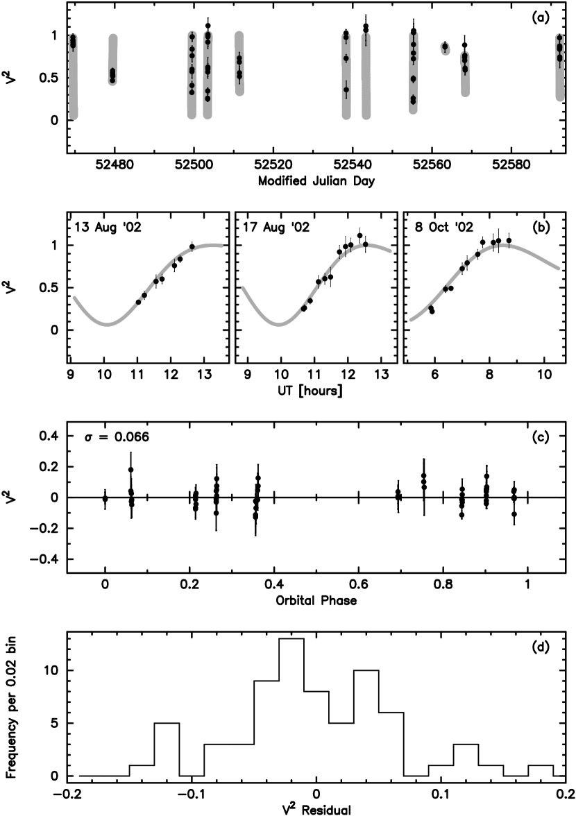
Figure 1:

Figure 2:

Figure 3:

Figure 4:

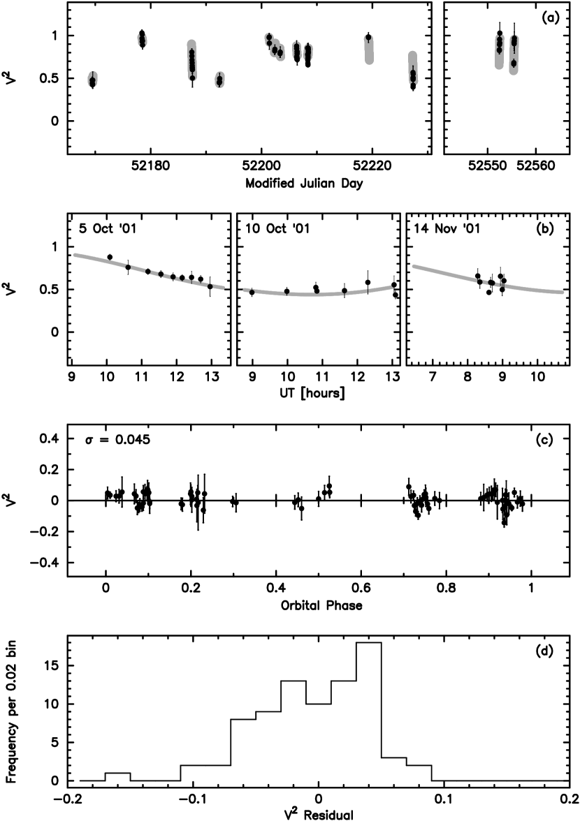
Figure 5:

Figure 6:

Figure 7:

Table 1: Calibration stars for HD 6118 and HD 27483

Target	Calibrator	Spectral	Magnitude	Angular Separation	Adopted
		Type		from Target (deg)	Diameter (mas)
HD 6118		B9.5V+B9.5V	5.5 V, 5.6 K
	HD 7034	F0V	5.2 V, 4.5 K	1.8	0.52$\pm$0.1
	HD 8673	F7V	6.3 V, 5.0 K	5.6	0.38$\pm$0.1
	HD 11007	F8V	5.8 V, 4.4 K	9.7	0.45$\pm$0.1
HD 27483		F6V+F6V	6.2 V, 5.1 K
	HD 21686	A0V	5.1 V, 5.1 K	12.6	0.32$\pm$0.09
	HD 24357	A4V	6.0 V, 5.0 K	7.5	0.40$\pm$0.09

Table 2: Best-fit Orbital Parameters for HD 6118

Parameter	HD 6118
Apparent semi-major axis, $\hat{a}$ (mas)	5.56 $\pm$ 0.04(0.03/0.03)
Period, $P$ (d)	81.12625 $\pm$ 2.7(2.0/1.7)$\times 10^{-4}$
Time of periastron, $T_{p}$ (MJD)	31308.153 $\pm$ 0.023(0.021/0.009)
Eccentricity, $e$	0.8956 $\pm$ 0.0020(0.0018/0.0008)
Longitude of the periastron, $\omega$ (deg)	346.6 $\pm$ 2.0(1.8/0.9)
Longitude of the ascending node, $\Omega$ (deg)	167.8 $\pm$ 1.7(1.5/0.7)
Inclination, $i$ (deg)	143.4 $\pm$ 1.3(1.0/0.7)
Brightness ratio (K band), $r_{K}$	0.69 $\pm$ 0.10(0.08/0.06)
Velocity amplitude of the primary, $K_{1}$ (km/s)	53.2 $\pm$ 1.9(1.9/0.3)
Velocity amplitude of the secondary, $K_{2}$ (km/s)	59.6 $\pm$ 1.6(1.6/0.1)
Systemic velocity, $\gamma$ (km/s)	10.5 $\pm$ 2.3(2.3/0.2)
Reduced $\chi^{2}$, $\chi^{2}/DOF$	1.06

Table 3: Physical Parameters for HD 6118

Parameter	Primary	Secondary
Semi-major axis, $a_{1,2}$ (AU)	0.296 $\pm$ 0.011(0.011/0.002)	0.332 $\pm$ 0.010(0.009/0.001)
Mass, $M$ (M⊙)	2.65 $\pm$ 0.27(0.23/0.16)	2.36 $\pm$ 0.24(0.21/0.12)
Parallax, $\kappa$ (mas)		$8.86\pm 0.07(0.05/0.04)$
Distance, $d$ (pc)		$112.9\pm 0.9$
Absolute K magnitude, $M_{K}^{2MASS}$ (mag)	0.92 $\pm$ 0.07	1.32 $\pm$ 0.10
Spectral type	B9.5V	B9.5V
Diameter, $\theta$ (mas)	0.16	0.15

Table 4: The K-band data set for HD 6118

MJD	$V^{2}$	$\sigma_{V^{2}}$	$(O-C)$	$\lambda$	$u$	$v$	Orbital
			($V^{2}$)	($\mu$m)	(m)	(m)	Phase
52469.4716	0.885	0.026	-0.111	2.206	-62.29763	-88.76658	0.844
52469.4750	0.943	0.044	-0.054	2.212	-61.59159	-89.46617	0.844
52469.4822	0.978	0.040	-0.012	2.216	-60.01158	-90.91343	0.844
52469.4896	0.937	0.024	-0.029	2.213	-58.23851	-92.37724	0.845
52469.4971	0.913	0.044	-0.015	2.213	-56.33916	-93.79407	0.845
52469.5043	0.896	0.033	0.020	2.209	-54.38969	-95.11475	0.845
52469.5114	0.879	0.066	0.055	2.215	-52.35453	-96.37247	0.845
52479.4491	0.467	0.026	-0.005	2.209	-80.25213	-6.10222	0.967
52479.4593	0.528	0.027	0.039	2.210	-81.60143	-8.83451	0.967
52479.4694	0.559	0.054	0.049	2.208	-82.60869	-11.58149	0.968
52479.4829	0.537	0.014	-0.007	2.212	-83.43723	-15.30779	0.968
52479.4964	0.583	0.031	0.001	2.208	-83.66175	-19.07214	0.968
52479.5097	0.520	0.068	-0.108	2.215	-83.28990	-22.75824	0.968
52499.4597	0.328	0.016	0.013	2.212	-83.02389	-24.03339	0.214
52499.4669	0.410	0.049	0.008	2.215	-82.46938	-26.01122	0.214
52499.4818	0.573	0.078	-0.012	2.218	-80.79138	-30.03950	0.214
52499.4894	0.601	0.056	-0.073	2.217	-79.65878	-32.06352	0.214
52499.5044	0.760	0.073	-0.066	2.213	-76.87996	-35.97718	0.214
52499.5115	0.837	0.041	-0.042	2.214	-75.33631	-37.76197	0.215
52499.5265	0.983	0.055	0.028	2.219	-71.56876	-41.42155	0.215
52503.4446	0.251	0.031	-0.007	2.213	-83.27129	-22.85984	0.263
52503.4459	0.260	0.039	-0.015	2.212	-83.20231	-23.21733	0.263
52503.4530	0.345	0.037	-0.030	2.211	-82.72204	-25.18546	0.263
52503.4635	0.569	0.075	0.042	2.212	-81.70878	-28.06198	0.263
52503.4712	0.605	0.064	-0.027	2.214	-80.74277	-30.13430	0.263
52503.4783	0.626	0.113	-0.100	2.213	-79.68035	-32.02812	0.263
52503.4898	0.921	0.077	0.076	2.219	-77.63532	-35.01885	0.264
52503.4970	0.984	0.119	0.076	2.215	-76.14014	-36.85894	0.264
52503.5037	1.004	0.081	0.051	2.211	-74.60828	-38.53705	0.264
52503.5149	1.114	0.091	0.123	2.213	-71.73623	-41.27522	0.264
52503.5219	1.010	0.096	0.012	2.223	-69.77414	-42.91569	0.264
52511.4097	0.733	0.067	-0.015	2.225	-48.33889	-98.55608	0.361
52511.4251	0.685	0.111	0.047	2.228	-43.21250	-100.88707	0.361
52511.4474	0.558	0.078	0.074	2.227	-35.01492	-103.79922	0.362
52511.4621	0.516	0.088	0.125	2.221	-29.24109	-105.36906	0.362
52538.3073	1.027	0.044	0.038	2.218	-82.52664	-11.31196	0.693
52538.3217	0.976	0.074	-0.001	2.217	-83.43361	-15.27362	0.693
52538.3450	0.729	0.046	0.008	2.214	-83.44924	-21.76152	0.693
52538.3663	0.360	0.103	0.004	2.218	-81.89032	-27.61842	0.694
52543.3030	1.062	0.122	0.103	2.224	-83.19274	-13.88360	0.754
52543.3044	1.110	0.108	0.143	2.222	-83.26775	-14.26941	0.754
52543.3201	1.060	0.182	0.067	2.224	-83.66703	-18.61957	0.755
52555.2441	0.259	0.038	0.012	2.226	-60.75089	-90.25274	0.902
52555.2458	0.219	0.032	-0.039	2.229	-60.36032	-90.60454	0.902
52555.2663	0.483	0.041	0.046	2.225	-55.25302	-94.54373	0.902
52555.2746	0.492	0.021	-0.020	2.227	-52.93196	-96.02605	0.902
52555.2915	0.724	0.068	0.055	2.224	-47.74311	-98.85137	0.902
52555.2994	0.792	0.084	0.051	2.218	-45.12403	-100.07088	0.902
52555.3155	0.893	0.058	0.040	2.223	-39.45833	-102.33171	0.902
52555.3230	1.035	0.065	0.140	2.225	-36.67357	-103.28025	0.903
52555.3393	1.032	0.102	0.069	2.228	-30.31187	-105.10536	0.903
52555.3470	1.053	0.140	0.070	2.227	-27.23835	-105.83424	0.903
52555.3630	1.055	0.087	0.058	2.230	-20.55383	-107.11264	0.903
52563.2452	0.875	0.038	-0.003	2.225	-55.07166	-94.66790	0.000
52563.2630	0.863	0.063	-0.011	2.223	-49.85921	-97.77326	0.000
52568.2017	0.741	0.092	0.043	2.235	-62.23040	-88.83121	0.061
52568.2086	0.886	0.112	0.180	2.238	-60.76237	-90.24129	0.061
52568.2242	0.703	0.108	-0.025	2.235	-57.00814	-93.30844	0.062
52568.2583	0.765	0.096	0.027	2.232	-46.96657	-99.22493	0.062
52568.3072	0.614	0.080	-0.047	2.240	-28.98546	-105.43060	0.063
52568.3265	0.591	0.041	-0.015	2.240	-20.99243	-107.04018	0.063
52592.1255	0.843	0.135	-0.110	2.228	-64.26670	-86.59406	0.356
52592.1271	0.837	0.102	-0.126	2.225	-63.98127	-86.93272	0.356
52592.1352	0.875	0.072	-0.115	2.228	-62.41920	-88.64280	0.356
52592.1472	0.972	0.041	-0.021	2.228	-59.81671	-91.08260	0.356
52592.1724	0.866	0.107	-0.023	2.230	-53.25580	-95.83075	0.357
52592.1741	0.854	0.032	-0.020	2.228	-52.77823	-96.12117	0.357
52592.1856	0.720	0.102	-0.069	2.227	-49.29094	-98.07232	0.357
52592.1877	0.745	0.031	-0.028	2.227	-48.61715	-98.41827	0.357

Table 5: Best-fit Orbital Parameters for HD 27483

Parameter	HD 27483
Period, $P$ (d)	3.0591080 $\pm$ 1.1(1.0/0.5)$\times 10^{-5}$
Time of periastron, $T_{p}$ (MJD)	44497.185696 $\pm$ 0.0026(0.0026/0.0006)
Eccentricity (assumed), $e$	0.0
Longitude of the ascending node, $\Omega$ (deg)	7.3 $\pm$ 3.6(3.2/1.7)
Inclination, $i$ (deg)	45.1 $\pm$ 1.7(0.6/1.6)
Brightness ratio (K band, assumed), $r_{K}$	1.0
Velocity amplitude of the primary, $K_{1}$ (km/s)	73.4 $\pm$ 0.4(0.4/0.03)
Velocity amplitude of the secondary, $K_{2}$ (km/s)	72.5 $\pm$ 0.6(0.6/0.07)
Systemic velocity, $\gamma$ (km/s)	39.2 $\pm$ 0.2(0.2/0.007)
Apparent semi-major axis, $\hat{a}$ (mas)	1.26 $\pm$ 0.05(0.05/0.0007)
Reduced $\chi^{2}$, $\chi^{2}/DOF$	1.3

Table 6: Physical Parameters for HD 27483

Parameter	Primary	Secondary
Semi-major axis, $a_{1,2}$ (AU)	0.02915 $\pm$ 1.4(1.4/0.1)$\times 10^{-4}$	0.02878 $\pm$ 2.4(2.4/0.3)$\times 10^{-4}$
Mass, $M$ (M⊙)	1.38 $\pm$ 0.13(0.05/0.12)	$\pm$ 1.39 0.13(0.05/0.12)
Parallax (from Hipparcos), $\kappa$ (mas)		$21.8\pm 0.85$
Distance (from Hipparcos), $d$ (pc)		$45.9\pm 1.8$
Absolute K magnitude, $M_{K}^{2MASS}$ (mag)	2.51 $\pm$ 0.07	2.51 $\pm$ 0.07
Spectral type	F6V	F6V
Diameter, $\theta$ (mas)	0.25	0.25

Table 7: The K-band data set for HD 27483

MJD	$V^{2}$	$\sigma_{V^{2}}$	$(O-C)$	$\lambda$	$u$	$v$	Orbital
			($V^{2}$)	($\mu$m)	(m)	(m)	Phase
52169.4411	0.477	0.038	0.049	2.216	-60.04103	-90.67138	0.004
52169.4617	0.442	0.020	0.034	2.211	-54.81478	-92.46702	0.011
52169.5040	0.425	0.035	0.028	2.217	-41.34146	-95.55666	0.025
52169.5256	0.432	0.044	0.028	2.214	-33.27606	-96.77422	0.032
52169.5473	0.478	0.097	0.055	2.219	-24.54295	-97.72336	0.039
52178.4216	1.031	0.037	0.038	2.206	-81.67179	-16.86810	0.940
52178.4457	0.966	0.070	-0.020	2.209	-83.47920	-19.87857	0.948
52178.4663	0.930	0.018	-0.046	2.211	-83.50226	-22.47998	0.954
52178.4863	1.015	0.028	0.053	2.212	-82.18878	-24.97510	0.961
52178.5066	0.936	0.039	-0.009	2.209	-79.51184	-27.46343	0.968
52178.5269	0.939	0.049	0.013	2.209	-75.54893	-29.83948	0.974
52178.5439	0.889	0.047	-0.020	2.208	-71.25532	-31.73276	0.980
52187.4202	0.806	0.041	0.013	2.214	-52.64961	-93.08626	0.881
52187.4419	0.761	0.085	0.021	2.219	-45.84172	-94.70129	0.888
52187.4660	0.714	0.039	0.037	2.220	-37.26240	-96.21923	0.896
52187.4814	0.681	0.044	0.043	2.218	-31.34041	-97.01585	0.901
52187.4957	0.647	0.049	0.044	2.216	-25.58201	-97.62907	0.906
52187.5065	0.622	0.036	0.044	2.217	-21.05021	-98.01201	0.910
52187.5179	0.623	0.070	0.069	2.219	-16.19633	-98.33250	0.913
52187.5288	0.601	0.044	0.069	2.218	-11.47321	-98.56032	0.917
52187.5401	0.503	0.108	-0.010	2.223	-6.51337	-98.71406	0.920
52192.3743	0.448	0.048	0.010	2.222	-60.93263	-90.30497	0.501
52192.4156	0.456	0.047	0.051	2.222	-49.91011	-93.78621	0.514
52192.4503	0.496	0.063	0.094	2.224	-38.05173	-96.09529	0.526
52192.4517	0.456	0.035	0.053	2.224	-37.50915	-96.17839	0.526
52201.3806	0.977	0.044	-0.011	2.214	-83.38707	-19.58007	0.445
52201.4042	0.983	0.044	0.006	2.211	-83.48201	-22.55729	0.453
52201.4276	0.911	0.074	-0.050	2.215	-81.75339	-25.48721	0.460
52202.3848	0.820	0.044	0.014	2.212	-83.60642	-20.45829	0.773
52202.4193	0.840	0.052	0.000	2.213	-82.32174	-24.80380	0.784
52203.3499	0.789	0.046	-0.017	2.215	-81.25220	-16.43679	0.089
52203.3879	0.806	0.063	0.051	2.215	-83.66799	-21.18956	0.101
52206.3447	0.877	0.064	0.042	2.214	-81.61656	-16.80890	0.068
52206.3551	0.848	0.041	0.029	2.220	-82.64579	-18.09778	0.071
52206.3660	0.755	0.042	-0.048	2.216	-83.34320	-19.45886	0.075
52206.3740	0.747	0.033	-0.046	2.218	-83.60796	-20.46804	0.077
52206.3844	0.750	0.041	-0.030	2.217	-83.63433	-21.78276	0.081
52206.3995	0.723	0.028	-0.042	2.223	-83.03426	-23.68374	0.085
52206.4086	0.812	0.041	0.056	2.220	-82.30747	-24.82260	0.088
52206.4217	0.790	0.061	0.043	2.221	-80.78114	-26.44374	0.093
52206.4352	0.787	0.043	0.047	2.216	-78.64555	-28.06514	0.097
52206.4404	0.811	0.057	0.072	2.216	-77.67525	-28.67474	0.099
52206.4541	0.731	0.076	-0.008	2.222	-74.68480	-30.26203	0.103
52206.4556	0.718	0.033	-0.020	2.217	-74.33879	-30.42443	0.104
52208.3170	0.854	0.054	0.089	2.215	-78.24352	-14.11855	0.712
52208.3315	0.779	0.041	0.026	2.214	-80.61362	-15.85313	0.717
52208.3500	0.779	0.028	0.034	2.212	-82.67478	-18.14216	0.723
52208.3576	0.712	0.028	-0.032	2.213	-83.19229	-19.08823	0.726
52208.3679	0.676	0.030	-0.070	2.219	-83.59498	-20.38941	0.729
52208.3772	0.730	0.038	-0.018	2.214	-83.65442	-21.57058	0.732
52208.3847	0.657	0.025	-0.095	2.213	-83.49330	-22.51368	0.734
52208.3982	0.759	0.035	-0.004	2.217	-82.73269	-24.21070	0.739
52208.4079	0.742	0.044	-0.030	2.214	-81.81728	-25.41565	0.742
52208.4150	0.788	0.028	0.008	2.215	-80.95680	-26.28502	0.744
52208.4261	0.834	0.030	0.039	2.216	-79.28248	-27.62896	0.748
52208.4362	0.855	0.056	0.044	2.219	-77.41629	-28.82800	0.751
52208.4398	0.838	0.059	0.022	2.219	-76.68183	-29.24409	0.752
52208.4507	0.811	0.032	-0.022	2.212	-74.20814	-30.48483	0.756
52208.4615	0.803	0.036	-0.051	2.220	-71.41482	-31.67054	0.760
52219.2873	0.984	0.033	-0.004	2.214	-63.61692	-89.06337	0.298
52219.3115	0.977	0.059	-0.013	2.213	-58.40521	-91.28894	0.306
52227.3454	0.568	0.078	0.002	2.231	-41.44225	-95.53847	0.933
52227.3478	0.506	0.067	-0.055	2.227	-40.59268	-95.68519	0.933
52227.3588	0.397	0.028	-0.143	2.229	-36.50589	-96.32982	0.937
52227.3610	0.496	0.054	-0.039	2.227	-35.68126	-96.44839	0.938
52227.3631	0.487	0.090	-0.045	2.228	-34.89705	-96.55776	0.938
52227.3726	0.550	0.092	0.036	2.227	-31.15997	-97.03593	0.941
52227.3746	0.419	0.064	-0.092	2.227	-30.36469	-97.12892	0.942
52227.3766	0.506	0.070	-0.002	2.228	-29.58014	-97.21776	0.943
52552.4301	0.834	0.045	0.056	2.221	-49.87012	-93.79909	0.200
52552.4378	0.826	0.042	0.027	2.222	-47.43702	-94.36073	0.203
52552.4707	0.894	0.044	0.009	2.223	-35.76859	-96.43770	0.214
52552.4788	0.956	0.046	0.052	2.221	-32.62244	-96.85885	0.216
52552.5181	0.913	0.081	-0.061	2.228	-16.42641	-98.32007	0.229
52552.5273	1.029	0.125	0.045	2.226	-12.45217	-98.52052	0.232
52555.4198	0.667	0.038	-0.021	2.227	-50.51831	-93.64104	0.178
52555.4276	0.683	0.042	-0.026	2.225	-48.07954	-94.21867	0.180
52555.4868	0.921	0.070	0.044	2.225	-26.13483	-97.57822	0.200
52555.4958	0.905	0.080	0.006	2.225	-22.41073	-97.90756	0.203
52555.5321	0.938	0.105	-0.031	2.227	-6.75279	-98.71059	0.214
52555.5430	0.969	0.177	-0.012	2.227	-1.96827	-98.78206	0.218

References

- Anderson (1920) Anderson, J. A. 1920, ApJ, 51, 263
- Armstrong et al. (1998) Armstrong, J. T. et al. 1998, ApJ, 496, 550
- Batten, Fletcher, & MacCarthy (1997) Batten, A. H., Fletcher, J. M., & MacCarthy, D. G. 1997, VizieR Online Data Catalog, 5064,
- Batten, Fletcher, & MacCarthy (1989) Batten, A. H., Fletcher, J. M., & MacCarthy, D. G. 1989, Publications of the Dominion Astrophysical Observatory Victoria, 17, 1
- Belserene (1947) Belserene, E. P. 1947, ApJ, 105, 229
- Bertelli et al. (1994) Bertelli, G., Bressan, A., Chiosi, C., Fagotto, F., & Nasi, E. 1994, A&AS, 106, 275
- Boden, Colavita, van Belle, & Shao (1998) Boden, A. F., Colavita, M. M., van Belle, G. T., & Shao, M. 1998, Proc. SPIE, 3350, 872
- Boden et al. (1999) Boden, A. F. et al. 1999, ApJ, 515, 356
- Boden et al. (1999) Boden, A. F. et al. 1999, ApJ, 527, 360
- Boden, Creech-Eakman, & Queloz (2000) Boden, A. F., Creech-Eakman, M. J., & Queloz, D. 2000, ApJ, 536, 880
- Boden (2000) Boden, A. F. 2000, Principles of Long Baseline Stellar Interferometry, 9
- Boden & Lane (2001) Boden, A. F. & Lane, B. F. 2001, ApJ, 547, 1071
- Born & Wolf (1999) Born, M. & Wolf, E. 1999, Principles of optics : electromagnetic theory of propagation, interference and diffraction of light / Max Born and Emil Wolf ; with contributions by A.B. Bhatia et al., Cambridge, England; New York: Cambridge University Press, 1999
- Campbell (1918) Campbell, W. W. 1918, PASP, 30, 351
- Colavita et al. (1999) Colavita, M. M. et al. 1999, ApJ, 510, 505
- Colavita (1999) Colavita, M. M. 1999, PASP, 111, 111
- Colavita & Wizinowich (2000) Colavita, M. M. & Wizinowich, P. L. 2000, Proc. SPIE, 4006, 310
- Cowley, Cowley, Jaschek, & Jaschek (1969) Cowley, A., Cowley, C., Jaschek, M., & Jaschek, C. 1969, AJ, 74, 375
- Cutri et al. (2003) Cutri, R. M. et al. 2003, VizieR Online Data Catalog, 2246
- Glindemann et al. (2000) Glindemann, A. et al. 2000, Proc. SPIE, 4006, 2
- Kamp (1967) van de Kamp, P. 1967, Principles of Astrometry, Freeman, San Francisco
- Koresko et al. (1998) Koresko, C. D. et al. 1998, ApJ, 509, L45
- Kovalevsky (1995) Kovalevsky, J. 1995, Modern Astrometry, Springer-Verlag Berlin Heidelberg New York, Astronomy and Astrophysics Library
- Johnson, MacArthur, & Mitchell (1968) Johnson, H. L., MacArthur, J. W., & Mitchell, R. I. 1968, ApJ, 152, 465
- Lane, Colavita, Boden, & Lawson (2000) Lane, B. F., Colavita, M. M., Boden, A. F., & Lawson, P. R. 2000, Proc. SPIE, 4006, 452
- Lebreton, Fernandes, & Lejeune (2001) Lebreton, Y., Fernandes, J., & Lejeune, T. 2001, A&A, 374, 540
- Mayor & Mazeh (1987) Mayor, M. & Mazeh, T. 1987, A&A, 171, 157
- McAlister et al. (2000) McAlister, H. A. et al. 2000, Proc. SPIE, 4006, 465
- Merrill (1922) Merrill, P. W. 1922, ApJ, 56, 40
- Michelson (1891) Michelson, A. A. 1891, Nature, 45, 160
- Mozurkewich et al. (1991) Mozurkewich, D. et al. 1991, AJ, 101, 2207
- Northcott & Wright (1952) Northcott, R. J. & Wright, K. O. 1952, JRASC, 46, 11
- Perryman et al. (1997) Perryman, M. A. C. et al. 1997, A&A, 323, L49
- Press, Teukolsky, Vetterling, & Flannery (1992) Press, W. H., Teukolsky, S. A., Vetterling, W. T., & Flannery, B. P. 1992, Cambridge: University Press
- Shao et al. (1988) Shao, M., Colavita, M. M., Hines, B. E., Staelin, D. H., & Hutter, D. J. 1988, A&A, 193, 357
- Shao & Colavita (1992) Shao, M. & Colavita, M. M. 1992, ARA&A, 30, 45
- Schwarzschild (1896) Schwarzschild, K. 1896, Astronomische Nachrichten, 139, 353
- Thompson, Moran, & Swenson (2001) Thompson, A. R., Moran, J. M., & Swenson, G. W. 2001, Interferometry and synthesis in radio astronomy by A. Richard Thompson, James M. Moran, and George W. Swenson, Jr. 2nd ed. New York : Wiley, c2001.xxiii, 692 p. : ill. ; 25 cm. ”A Wiley-Interscience publication.” Includes bibliographical references and indexes. ISBN : 0471254924
- Torres et al. (2002) Torres, G., Boden, A. F., Latham, D. W., Pan, M., & Stefanik, R. P. 2002, AJ, 124, 1716
- Quirrenbach (2001) Quirrenbach, A. 2001, ARA&A, 39, 353