The Three-Dimensional Power Spectrum of Galaxies from the Sloan Digital Sky Survey

Abstract

We measure the large-scale real-space power spectrum $P(k)$ using a sample of 205,443 galaxies from the Sloan Digital Sky Survey, covering 2417 effective square degrees with mean redshift $z\approx 0.1$. We employ a matrix-based method using pseudo-Karhunen-Loève eigenmodes, producing uncorrelated minimum-variance measurements in 22 $k$-bands of both the clustering power and its anisotropy due to redshift-space distortions, with narrow and well-behaved window functions in the range $0.02\,h/{\rm Mpc}<k<0.3\,h/{\rm Mpc}$. We pay particular attention to modeling, quantifying and correcting for potential systematic errors, nonlinear redshift distortions and the artificial red-tilt caused by luminosity-dependent bias. Our results are robust to omitting angular and radial density fluctuations and are consistent between different parts of the sky. Our final result is a measurement of the real-space matter power spectrum $P(k)$ up to an unknown overall multiplicative bias factor. Our calculations suggest that this bias factor is independent of scale to better than a few percent for $k<0.1\,h/{\rm Mpc}$, thereby making our results useful for precision measurements of cosmological parameters in conjunction with data from other experiments such as the WMAP satellite. The power spectrum is not well-characterized by a single power law, but unambiguously shows curvature. As a simple characterization of the data, our measurements are well fit by a flat scale-invariant adiabatic cosmological model with $h\Omega_{m}=0.213\pm 0.023$ and $\sigma_{8}=0.89\pm 0.02$ for $L_{*}$ galaxies, when fixing the baryon fraction $\Omega_{b}/\Omega_{m}=0.17$ and the Hubble parameter $h=0.72$; cosmological interpretation is given in a companion paper.

Σ

Department of Physics, University of Pennsylvania, Philadelphia, PA 19101, USA Center for Cosmology and Particle Physics, Department of Physics, New York University, 4 Washington Place, New York, NY 10003 Princeton University Observatory, Princeton, NJ 08544, USA Department of Physics, Drexel University, Philadelphia, PA 19104, USA Department of Astronomy, Ohio State University, Columbus, OH 43210, USA Fermi National Accelerator Laboratory, P.O. Box 500, Batavia, IL 60510, USA Center for Cosmological Physics and Department of Astronomy & Astrophysics, University of Chicago, Chicago, IL 60637, USA Department of Physics and Astronomy, The Johns Hopkins University, 3701 San Martin Drive, Baltimore, MD 21218, USA University of Pittsburgh, Department of Physics and Astronomy, 3941 O’Hara Street, Pittsburgh, PA 15260, USA Department of Astronomy, University of Arizona, Tucson, AZ 85721, USA JILA and Dept. of Astrophysical and Planetary Sciences, U. Colorado, Boulder, CO 80309, USA, Andrew.Hamilton@colorado.edu Department of Physics, 5000 Forbes Avenue, Carnegie Mellon University, Pittsburgh, PA 15213, USA Institute for Astronomy, University of Hawaii, 2680 Woodlawn Drive, Honolulu, HI 96822, USA Apache Point Observatory, 2001 Apache Point Rd, Sunspot, NM 88349-0059, USA Dept. of Physics, Massachusetts Institute of Technology, Cambridge, MA 02139 Institut d’Estudis Espacials de Catalunya/CSIC, Gran Capita 2-4, 08034 Barcelona, Spain Sussex Astronomy Centre, University of Sussex, Falmer, Brighton BN1 9QJ, UK Inst. for Cosmic Ray Research, Univ. of Tokyo, Kashiwa 277-8582, Japan U.S. Naval Observatory, Flagstaff Station, Flagstaff, AZ 86002-1149, USA Dept. of Physics, Univ. of Michigan, Ann Arbor, MI 48109-1120, USA Physics Dept., Rochester Inst. of Technology, 1 Lomb Memorial Dr, Rochester, NY 14623, USA Dept. of Astronomy and Astrophysics, Pennsylvania State University, University Park, PA 16802, USA Enrico Fermi Institute, University of Chicago, Chicago, IL 60637, USA

1. Introduction

The spectacular recent cosmic microwave background (CMB) measurements from the WMAP satellite (Bennett et al. 2003) and other experiments have increased the importance of non-CMB measurements for the endeavor to constrain cosmological models and their free parameters. These non-CMB constraints are crucially needed for breaking CMB degeneracies (Eisenstein et al. 1999; Efstathiou & Bond 1999; Bridle et al. 2003); for instance, WMAP alone is consistent with a closed universe with Hubble parameter $h=0.32$ and no cosmological constant (Spergel et al. 2003; Verde et al. 2003). Yet they are currently less reliable and precise than the CMB, making them the limiting factor and weakest link in the quest for precision cosmology. Much of the near-term progress in cosmology will therefore be driven by reductions in statistical and systematic uncertainties of non-CMB probes such as Lyman $\alpha$ forest and galaxy clustering and motions, gravitational lensing, cluster studies, and supernovae Ia distance determinations. Galaxy redshift surveys can play a key role in breaking degeneracies and providing cross checks (Tegmark 1997a; Goldberg & Strauss 1998; Wang et al. 1999; Eisenstein et al. 1999), but only if systematics can be controlled to high precision. The goal of the present paper is to do just this, using over 200,000 galaxies from the Sloan Digital Sky Survey (SDSS; York et al. 2000) to measure the shape of the real-space matter power spectrum $P(k)$, accurately quantifying and correcting for the effects of light-to-mass bias, redshift space distortions, survey geometry effects and other complications.

The cosmological constraining power of three-dimensional maps of the Universe provided by galaxy redshift surveys has motivated ever more ambitious observational efforts such as the CfA/UZC (Huchra et al. 1990; Falco et al. 1999), LCRS (Shectman et al. 1996), and PSCz (Saunders et al. 2000) surveys, each well in excess of $10^{4}$ galaxies. The current state of the art is the AAT two degree field galaxy redshift survey (2dFGRS; Colless et al. 2001; Hawkins et al. 2003; Peacock 2003 and references therein). Analysis of the first 147,000 2dFGRS galaxies (Peacock et al. 2001; Percival et al. 2001, 2002; Norberg et al. 2001, 2002; Madgwick et al. 2002) have supported a flat dark-energy dominated cosmology, as have angular clustering analyses of the parent catalogs underlying the 2dFGRS (Efstathiou & Moody 2001) and SDSS (Scranton et al. 2002; Connolly et al. 2002; Tegmark et al. 2002; Szalay et al. 2003; Dodelson et al. 2002). Tantalizing evidence for baryonic wiggles in the galaxy power spectrum is presented by Percival et al. (2001) and Miller et al. (2001a,b, 2002), and cosmological models have been further constrained in conjunction with cosmic microwave background (CMB) data (e.g., Spergel et al. 2003; Verde et al. 2003; Lahav et al. 2002).

The SDSS is the most ambitious galaxy redshift survey to date, whose goal, driven by large-scale structure science, is to measure of order $10^{6}$ galaxy redshifts. Zehavi et al. (2002) computed the correlation function using about 30,000 galaxies from early SDSS data (Stoughton et al. 2002). In conjunction with the first major SDSS data release in 2003 (hereafter DR1; Abazajian et al. 2003), a series of papers will address various aspects of the 3D clustering of a much larger data set involving over 200,000 galaxies with redshifts. This paper is focused on measuring the power galaxy spectrum $P(k)$ on large scales, dealing with complications such as luminosity-dependent bias and redshift distortions only to the extent necessary to recover an undistorted measurement of the real-space matter power spectrum. Zehavi et al. (2003a) measure and model the real space correlation function, mainly on smaller scales, focusing on departures from power-law behavior, and Zehavi et al. (2003b) will study how the correlation function depends on galaxy properties. Pope et al. (2003) measure the parameters which characterize the large-scale power spectrum with a complementary approach involving direct likelihood analysis on Karhunen-Loève eigenmodes, as opposed to the quadratic estimator technique employed in the present paper.

This paper is organized as follows. In Section 2, we describe the SDSS data used and how we model it; the technical details can be found in Appendix A. In Section 3, we describe our methodology and present our basic measurements of both the power spectrum and its redshift-space anisotropy. The details of the formalism for doing this are described in Appendix B. In Section 4 we focus on this anisotropy to model, quantify and correct for the effects of redshift-space distortions, producing an estimate of the real-space galaxy power spectrum and testing our procedure with Monte-Carlo simulations. In Section 5, we model, quantify and correct for the effects of luminosity-dependent biasing, producing an estimate of the real-space matter power spectrum. In Section 6, we test for a variety of systematic errors. In Section 7, we discuss our results. The cosmological interpretation of our measurements is given in a companion paper (Tegmark et al. 2003, hereafter “Paper II”).

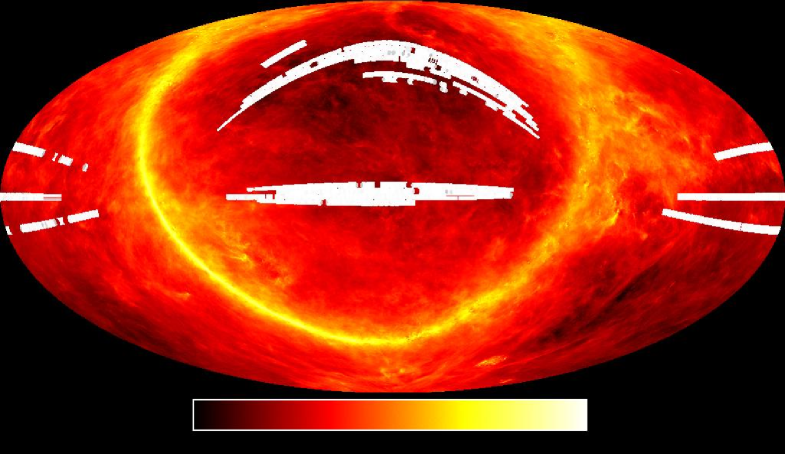
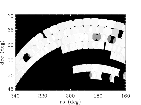
Figure 1.— The upper panel shows the angular completeness map, the relative probabilities that galaxies in various directions get included, in Hammer-Aitoff projection in equatorial coordinates on a grayscale ranging from black (0) to white (1). It is this completeness map that we expand in spherical harmonics. The backdrop is the logarithm of the dust map from Schlegel, Finkbeiner, & Davis (1998), indicating which sky regions are most likely to be affected by extinction-related systematic errors. The lower panel illustrates the complex nature of the completeness map and the high average completeness with a zoom of a small sky region.

2. Data and data modeling

The SDSS uses a mosaic CCD camera (Gunn et al. 1998) to image the sky in five photometric bandpasses denoted $u$, $g$, $r$, $i$, $z$ (Fukugita et al. 1996). After astrometric calibration (Pier et al. 2003), photometric data reduction (Lupton et al. 2003, in preparation; see Lupton et al. 2001 and Stoughton et al. 2002 for summaries) and photometric calibration (Hogg et al. 2001; Smith et al. 2002), galaxies are selected for spectroscopic observations using the algorithm described by Strauss et al. (2002). To a good approximation, the main galaxy sample consists of all galaxies with $r$-band apparent Petrosian magnitude $r<17.77$; see Appendix A. Galaxy spectra are also measured for a luminous red galaxy sample (Eisenstein et al. 2001), for which clustering results will be reported in a separate paper. These targets are assigned to spectroscopic plates by an adaptive tiling algorithm (Blanton et al. 2003) and observed with a pair of fiber-fed CCD spectrographs (Uomoto et al., in preparation), after which the spectroscopic data reduction and redshift determination are performed by automated pipelines (Schlegel et al., in preparation; Frieman et al., in preparation). The rms galaxy redshift errors are $\sim$ 30 km/s and hence negligible for the purpose of the present paper.

Our analysis is based on SDSS sample11 (Blanton et al. 2003c), consisting of the 205,443 galaxies observed before July 2002, all of which will be included in the upcoming SDSS Data Release 2. From this basic sample, we produce a set of subsamples as specified in Table 1. The details of how this basic sample was processed, modeled and subdivided are given in Appendix A. The bottom line is that each sample is completely specified by three entities:

1. The galaxy positions (a list of RA, Dec and comoving redshift space distance $r$ for each galaxy)

2. The radial selection function ${\bar{n}}(r)$, which gives the expected (not observed) number density of galaxies as a function of distance

3. The angular selection function ${\bar{n}}(\widehat{\bf r})$, which gives the completeness as a function of direction in the sky

Our samples are constructed so that their three-dimensional selection function is separable, i.e., simply the product ${\bar{n}}({\bf r})={\bar{n}}(\widehat{\bf r}){\bar{n}}(r)$ of an angular and a radial part; here $r\equiv|{\bf r}|$ and $\widehat{\bf r}\equiv{\bf r}/r$ are the comoving radial distance and the unit vector corresponding to the position ${\bf r}$. The conversion from redshift $z$ to comoving distance was made for a flat cosmological model with a cosmological constant $\Omega_{\Lambda}=0.7$ — below we will see that our results are insensitive to this assumption.

Table 1 – The table summarizes the various galaxy samples used in our analysis, listing cuts made on evolution-corrected absolute magnitude $M_{{{}^{0.1}\!{r}}}$ (for $h=1$), apparent magnitude $r$ and redshift $z$. $M_{{{}^{0.1}\!{r}}}$ was computed from $r$ and $z$ assuming a flat cosmological model with $\Omega_{\Lambda}=0.7$.

Sample name	Abs. mag	App. mag	Redshift	Sq. degrees	Galaxies
all	All	$r<17.5-17.77$	All	2417	205,443
safe0	All	$14.50<r<17.50$	All	2417	157,389
safe13	$-23<M_{{{}^{0.1}\!{r}}}<-18.5$	$14.50<r<17.50$	$0.001<z<0.400$	2417	146,633
safe22	$-22<M_{{{}^{0.1}\!{r}}}<-19.0$	$14.50<r<17.50$	$0.001<z<0.400$	2417	134,674
baseline	$-23<M_{{{}^{0.1}\!{r}}}<-18.5$	$14.50<r<17.50$	$0.002<z<0.210$	2417	143,314
Angular subsamples:
A1 (south)	$-23<M_{{{}^{0.1}\!{r}}}<-18.5$	$14.50<r<17.50$	$0.017<z<0.210$	600	35,782
A2 (north)	$-23<M_{{{}^{0.1}\!{r}}}<-18.5$	$14.50<r<17.50$	$0.017<z<0.210$	1817	107,532
A3 (north eq)	$-23<M_{{{}^{0.1}\!{r}}}<-18.5$	$14.50<r<17.50$	$0.017<z<0.210$	809	52,081
A4 (north rest)	$-23<M_{{{}^{0.1}\!{r}}}<-18.5$	$14.50<r<17.50$	$0.017<z<0.210$	1007	55,451
Radial subsamples:
R1 (near)	$-23<M_{{{}^{0.1}\!{r}}}<-18.5$	$14.50<r<17.50$	$0.017<z<0.078$	2417	47,954
R2 (mid)	$-23<M_{{{}^{0.1}\!{r}}}<-18.5$	$14.50<r<17.50$	$0.078<z<0.117$	2417	47,089
R3 (far)	$-23<M_{{{}^{0.1}\!{r}}}<-18.5$	$14.50<r<17.50$	$0.117<z<0.210$	2417	48,271
Luminosity (volume-limited) subsamples:
L1	$-17<M_{{{}^{0.1}\!{r}}}<-16$	$14.50<r<17.50$	$0.008<z<0.017$	2417	455
L2	$-18<M_{{{}^{0.1}\!{r}}}<-17$	$14.50<r<17.50$	$0.011<z<0.027$	2417	1,736
L3	$-19<M_{{{}^{0.1}\!{r}}}<-18$	$14.50<r<17.50$	$0.017<z<0.042$	2417	5,191
L4	$-20<M_{{{}^{0.1}\!{r}}}<-19$	$14.50<r<17.50$	$0.027<z<0.065$	2417	14,356
L5	$-21<M_{{{}^{0.1}\!{r}}}<-20$	$14.50<r<17.50$	$0.042<z<0.103$	2417	31,026
L6	$-22<M_{{{}^{0.1}\!{r}}}<-21$	$14.50<r<17.50$	$0.065<z<0.157$	2417	24,489
L7	$-23<M_{{{}^{0.1}\!{r}}}<-22$	$14.50<r<17.50$	$0.104<z<0.238$	2417	3,594
L8	$-24<M_{{{}^{0.1}\!{r}}}<-23$	$14.50<r<17.50$	$0.164<z<0.349$	2417	95
Mock samples:
M1-M275 (PThalos)			$0.015<z<0.240$	1395	108,300
V1-V10 (VIRGO)			$0.001<z<0.150$	1139	103,400

2.1. Angular selection function

The angular selection function ${\bar{n}}(\widehat{\bf r})$ is shown in Figure 1. For the baseline sample, it covers a sky area of 2499 square degrees. The function ${\bar{n}}(\widehat{\bf r})$ is defined to be the completeness, i.e., the probability that a galaxy satisfying the sample cuts actually gets assigned a redshift (including the 6% of the total which are determined based on the nearest neighbor redshift as described in Appendix A). Therefore the completeness is a dimensionless number between zero and one. The effective area is $\int{\bar{n}}(\widehat{\bf r})d\Omega\approx 2417$ square degrees, corresponding to an average completeness of $96.7\%$. As detailed in Appendix A.2, we model ${\bar{n}}(\widehat{\bf r})$ as a piecewise constant function. We specify this function by giving its value in each of a large number of disjoint spherical polygons, within each of which it takes a constant value. There are 2914 such polygons for the baseline sample, encoding the geometric boundaries of spectroscopic tiles, holes and other relevant entities. Figure 1 shows that the sky coverage naturally separates into three fairly compact regions of comparable size: north of the Galactic plane (in the center of the figure), there is one region on the celestial equator and another at high declination; south of the Galactic plane, there is a set of three stripes near the equator. For the purpose of testing for systematic errors, we define angular subsamples A1, A3 and A4 corresponding to these regions (see Table 1), which have effective areas of 809, 1007 and 600 square degrees, respectively.

2.2. Radial selection function

Our estimate of the radial selection function for the baseline sample is shown in Figure 2, together with a histogram of the galaxy distances. The full details of the derivation of the radial selection function can be found in Appendix A.4, including both evolution and K-corrections. Our basic sample has magnitude limits $r\geq 14.5$ at the bright end (since the survey becomes incomplete for bright galaxies with large angular size) and $r\leq 17.5$ at the faint end (Appendix A.4).

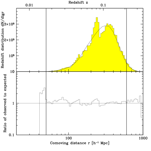
Figure 2.— The redshift distribution of the galaxies in sample safe13 is shown as a histogram and compared with the expected distribution in the absence of clustering, $\ln 10{\bar{n}}(r)r^{3}d\Omega$ (solid curve) in comoving coordinates assuming a flat $\Omega_{\Lambda}=0.7$ cosmology. The bottom panel shows the ratio of observed and expected distributions. The vertical lines indicate the redshift limits ($50\,h^{-1}{\rm Mpc}<r<600\,h^{-1}{\rm Mpc}$) employed in the baseline analysis. This near cut removes only 22 galaxies, the far cut 3295.

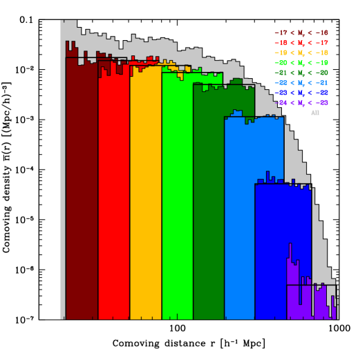
Figure 3.— Same as Figure 2 but plotted as comoving number density. The grey (background) histogram shows the full flux-limited sample and the others show the volume-limited subsamples, with lines indicating their predicted constant selection functions.

Figure 4 shows all galaxies within $5^{\circ}$ of the equator in a pie diagram, color coded by their absolute magnitude, and illustrates one of the fundamental challenges for our project (and indeed for the analysis of any flux-limited sample): luminous galaxies dominate the sample at large distances and dim ones dominate nearby. A measurement of the power spectrum on very large scales is therefore statistically dominated by luminous galaxies whereas a measurement on small scales is dominated by dim ones (since they have much higher number density). Yet it is well-known that luminous galaxies cluster more than dim ones (e.g., Davis et al. 1988; Hamilton 1988; Norberg et al. 2001; Zehavi et al. 2002; Verde et al. 2003), so when comparing $P(k)$ on large and small scales we are in effect comparing apples with oranges, and may mistakenly conclude that the power spectrum is red-tilted (with a spectral index $n=0.94$, say) even if the truth is $n=1$. So far, no magnitude-limited galaxy power spectrum analysis has been corrected for this effect. We do so in Section 5. Although this effect is is not large in an absolute sense, we find that it must nonetheless be included for precision cosmology applications.

The first step is to quantify the luminosity-dependence of bias. For this purpose, we define a series of volume-limited samples as specified in Table 1, constructed by discarding all galaxies that are too faint to be included at the far limit or too bright to be included at the near limit. This gives a radial selection function (Figure 3) that is constant within the radial limits and zero elsewhere. The radial limits are set so that galaxies at the far (near) radial limit and the dim (luminous) end of the absolute magnitude range in question have fluxes at the faint (bright) flux limits, respectively. Because the flux range $14.5<r<17.5$ spans exactly three magnitudes, these subsamples overlap spatially only with their nearest neighbor samples, and have a near limit that would be equal to the far limit of the sample that is two notches more luminous if it were not for evolution and K-corrections. This is clear in Figures 5 and 6. These samples have the advantage that the measured clustering is that of a well-defined set of objects whose selection is redshift-independent. Although we have not accounted for our surface brightness limits in defining these samples, very few of even the lowest luminosity galaxies in our sample are affected by the surface-brightness limits of the survey (Blanton et al. 2002c; Strauss et al. 2002).

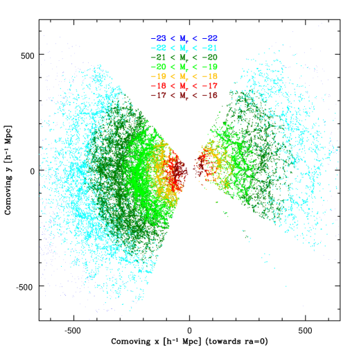
Figure 4.— The distribution of 67,676 galaxies within $5^{\circ}$ of the Equatorial plane, color coded by their absolute magnitudes. $M_{r}$ in the figure refers to the absolute $r$-magnitude $K$-corrected to $z=0.1$.

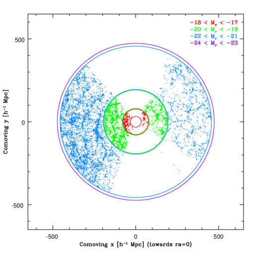
Figure 5.— The distribution of galaxies within $5^{\circ}$ of the equatorial plane is shown for the volume-limited subsamples L1, L3, L5 and L7 from Table 1.

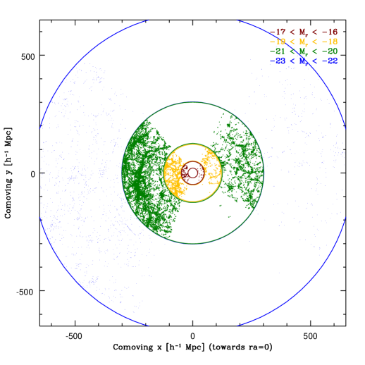
Figure 6.— The distribution of galaxies within $5^{\circ}$ of the equatorial plane is shown for the remaining four volume-limited subsamples from Table 1, i.e., L2, L4, L6 and L8.

3. Method and basic analysis

We now turn to our basic goal: accurately measuring the shape of the matter power spectrum $P(k)$ on large scales using the data described above, i.e., measuring a curve that equals the large-scale matter power spectrum up to an unknown overall multiplicative bias factor that is independent of scale. This involves four basic challenges:

1. Accounting for the complicated survey geometry

2. Correcting for the effect of redshift-space distortions

3. Correcting for bias effects, which as described in Section 5 cause an artificial red-tilt in the power spectrum

4. Checking for potential systematic errors

Before delving into detail, let us summarize each of these challenges and how we will tackle them.

3.1. Battle plan

3.1.1 Survey geometry and method of estimating power

It is well-known that since galaxies in a redshift survey probe the underlying density field only in a finite volume, the power spectrum estimated with traditional Fourier methods (e.g., Percival et al. 2001; Feldman, Kaiser & Peacock 1994), is complicated to interpret: it corresponds to a smeared-out version of the true power spectrum, can underestimate power on the largest scales due to the so-called integral constraint (Peacock & Nicholson 1991) and has correlated errors. We therefore measure power spectra with an alternative, matrix-based approach which, although more numerically demanding, has several advantages on the large scales that are the focus of this paper. It facilitates tests for radial and angular systematic errors. If galaxies were faithful tracers of mass, then it would produce unbiased minimum-variance power spectrum measurements with uncorrelated error bars that are smaller than those from traditional Fourier methods. The power smearing is quantified by window functions that are both narrower than with traditional Fourier methods and can be computed without need for approximations or Monte-Carlo simulations. (We do, however, use Monte Carlo simulations in Section 4 to verify that the method and software work as advertised.)

3.1.2 Redshift space distortions

Our basic input data consist of galaxy positions ${\bf r}$ in three-dimensional “redshift space”, where the comoving distance $r=|{\bf r}|$ is that which would explain the observed redshift if the galaxy were merely following the Hubble flow of the expanding Universe. The same gravitational forces that cause galaxies to cluster also cause them to move relative to the Hubble flow, and these so-called peculiar velocities make the clustering in redshift space anisotropic (Kaiser 1987; Hamilton 1998). Although this effect can be modeled and accounted for exactly on very large scales on which the clustering is linear (Kaiser 1987), nonlinear corrections cannot be neglected on some of the scales of interest to us (Scoccimarro et al. 2001; Seljak 2001; Cole et al. 1994; Hatton & Cole 1998). Section 4 is devoted to dealing with this complication, going beyond the Kaiser approximation with a three-pronged approach:

1. We precede our power spectrum analysis by a nonlinear “finger-of-God” compression step with a tunable threshold, to quantify the sensitivity of our results to nonlinear galaxy groups and clusters.

2. We measure three power spectra (galaxy-galaxy, galaxy-velocity and velocity-velocity spectra) rather than one, quantifying the clustering anisotropy and allowing the real-space power to be reconstructed beyond linear order.

3. We analyze an extensive set of mock galaxy catalogs to quantify the accuracy of our results and measure how the non-linear correction factor grows toward smaller scales.

Our mock analysis will also allow us to quantify the effects of nonlinear clustering on the error bars and band-power correlations. Step 1 is optional, and we present results both with and without it.

3.1.3 Bias

All we can ever measure with galaxy redshift surveys is galaxy clustering, whereas what we care about for constraining cosmological models is the clustering of the underlying matter distribution. Our ability to do cosmology with the real-space galaxy power spectrum $P_{\rm gg}(k)$ is therefore only as good as our understanding of bias, i.e., the relation of $P_{\rm gg}(k)$ to the matter power spectrum $P(k)$. Pessimists have often argued that since we do not understand galaxy formation at high precision, we cannot understand bias accurately either, and so galaxy surveys will be relegated to a historical footnote, having no role to play in the precision cosmology era. Optimists retort that no matter how complicated the gas-dynamical and radiative processes involved in galaxy formation may be, they have only a finite spatial range (a few $h^{-1}$Mpc, say), leading to a generic prediction that bias on much larger scales ($>20h^{-1}$Mpc, say) should be scale-independent for any particular type of galaxy (Coles 1993; Fry and Gaztañaga 1993; Scherrer & Weinberg 1998; Mann, Peacock & Heavens 1998; Coles, Melott & Munshi 1999; Heavens, Matarrese & Verde 1999; Blanton et al. 2000; Narayanan et al. 2000). This theoretical expectation is supported by visual inspection of the galaxy distribution. Comparing early and late type galaxies in the 2dF galaxy redshift survey (Peacock 2003; Madgewick et al. 2003) shows that whereas the small-scale distribution differs (ellipticals display a more “skeletal” distribution than do cluster-shunning spirals), their large-scale clustering patterns are indistinguishable.

We will devote Section 5 to the bias issue, arguing that both the pessimists and the optimists have turned out to be right: yes, biasing is indeed complicated on small scales (where the galaxy power spectrum will therefore teach us more about galaxy formation than about cosmology) but no, this in no way prevents us from doing precision cosmology with the galaxy power spectrum on very large scales. Our main tool will be analyzing our volume-limited magnitude subsamples, showing that their large-scale power spectra are consistent with all having the same shape and differing merely in amplitude.

Although the argument above for scale-independent bias holds only for a volume-limited subsample, we wish to use our full galaxy sample over a broad range of redshifts, both to expand the range of $k$-scales probed and to reduce shot noise. We will therefore use our measured luminosity-dependence of bias to compute and remove the artificial red tilt in our full magnitude-limited baseline sample.

In future papers, we will constrain galaxy bias empirically using clustering measurements on smaller scales (e.g., Zehavi et al. 2003), which will allow us to calculate the effects of scale-dependent bias on the power spectrum in the non-linear regime, and thus to extend the measurement of the matter power spectrum shape to smaller scales.

3.1.4 Systematic errors

As the old saying goes, the devil you know poses a lesser threat than the devil you don’t. We will therefore devote Section 6 to testing for the sort of effects that are not included in our Monte Carlo simulations. This includes both radial modulations (due to mis-estimates of evolution or $K$-corrections) and angular modulations (due to effects such as uncorrected dust extinction, variable observing conditions, photometric calibration errors and fiber collisions). Our tests use two basic approaches:

1. Analyzing subsets of galaxies: we compare the power spectra from different parts of the sky (subsamples A1-A4 from Table 1) and different distance ranges (subsamples R1-R3) looking for inconsistencies.

2. Analyzing subsets of modes: we look for excess power in purely angular and purely radial modes of the density field, which act like lightning rods for angular and radial modulations such as those mentioned above.

3.2. Three Step Power Spectrum Estimation

Our matrix-based power spectrum estimation approach is described in Tegmark et al. (1998). It starts by expanding the galaxy density field in a set of functions known as Pseudo-Karhunen-Loève eigenmodes. This step compresses the data set into a much smaller size (from hundreds of thousands of galaxy coordinates to a few thousand expansion coefficients) while retaining the large-scale cosmological information in which we are interested. It also reduces the power spectrum estimation problem to a mathematical form equivalent to that encountered in CMB analysis, enabling us to take advantage of a powerful set of matrix-based tools that have been fruitfully employed in the CMB field. Our basic analysis in the remainder of this section therefore consists of the following three steps:

1. Finger-of-god compression to remove redshift-space distortions due to virialized structures; Section 3.3

2. Pseudo-Karhunen-Loève eigenmode expansion; § 3.4

3. Power spectrum estimation using quadratic estimators; § 3.6.

As mentioned, the third step measures not one but three power spectra, encoding clustering anisotropy that contains information about redshift space distortions. In this section, we merely present the basic measurement of these three curves, which involves no assumptions about linearity, the nature of biasing or anything else. We then return to modeling and interpreting these curves in terms of real-space power in Section 4 and to bias modeling in Section 5.

     

Figure 7.— The effect of our Finger-of-god (FOG) removal is shown in part of the equatorial slice $|\delta|<5^{\circ}$ before (left) and after (right) FOG compression. Top panels show all 67,626 galaxies in the slice, bottom panels show the 28,255 that are identified as belonging to FOGs (with density threshold 200).

3.3. Step 1: Finger-of-god compression

Since our analysis method is motivated by (although not limited to) the linear Kaiser approximation for redshift space distortions, it is crucial that we are able to empirically quantify our sensitivity to the so-called finger-of-god (FOG) effect whereby radial velocities in virialized clusters make them appear elongated along the line of sight. We therefore start our analysis by compressing (isotropizing) FOGs, as illustrated in Figure 7. The FOG compression involves a tunable threshold density, and in Section 4 we will study how the final results change as we gradually change this threshold to include lesser or greater numbers of FOGs.

We use a standard friends-of-friends algorithm, in which two galaxies are considered friends, therefore in the same cluster, if the density windowed through an ellipse 10 times longer in the radial than transverse directions, centered on the pair, exceeds a certain overdensity threshold. To avoid linking well-separated galaxies in deep, sparsely sampled parts of the survey, we impose the additional constraint that friends should be closer than $r_{\perp\max}=5\,h^{-1}{\rm Mpc}$ in the transverse direction. The two conditions are combined into the following single criterion: two galaxies separated by $r_{\parallel}$ in the radial direction and by $r_{\perp}$ in the transverse direction are considered friends if

$$\left[(r_{\parallel}/10)^{2}+r_{\perp}^{2}\right]^{1/2}\leq\left[{4\over 3}\pi{\bar{n}}(1+\delta_{c})+r_{\perp\max}^{-3}\right]^{-1/3}$$ (1)

where ${\bar{n}}$ is the 3D selection function at the position of the pair, and $\delta_{c}$ is an overdensity threshold. Note that $\delta_{c}$ represents not the overdensity of the pair as seen in redshift space, but rather the overdensity of the pair after their radial separation has been reduced by a factor of 10. Thus $\delta_{c}$ is intended to approximate the threshold overdensity of a cluster in real space. We have chosen $r_{\perp\max}$ somewhat larger than the virial diameter of typical clusters to be conservative, minimizing the risk of missing FOGs — for our baseline threshold $\delta_{c}=200$, our results are essentially unaffected by this choice of $r_{\perp\max}$. Having identified a cluster by friends-of-friends in this fashion, we measure the dispersion of galaxy positions about the center of the cluster in both radial and transverse directions. If the one-dimensional radial dispersion exceeds the transverse dispersion, then the cluster is deemed a FOG, and the FOG is then compressed radially so that the cluster becomes round, that is, the transverse dispersion equals the radial dispersion. We perform the entire analysis five times, using density cutoffs $1{+}\delta_{c}=\infty$, 200, 100, 50 and 25, respectively; in our analyses below, we will explore the sensitivity of our results to this cutoff. The infinite threshold $1{+}\delta_{c}=\infty$ corresponds to no compression at all.

Figure 7 illustrates FOG compression with threshold density $1{+}\delta_{c}=200$, and unless explicitly stated otherwise, all results presented in this paper are for this threshold density. We make this choice to be on the safe side: Bryan & Norman (1998) estimate that the overdensity of a cluster at virialization is about 337 in a $\Lambda$CDM model, rising further as the Universe expands and the background density continues to drop.

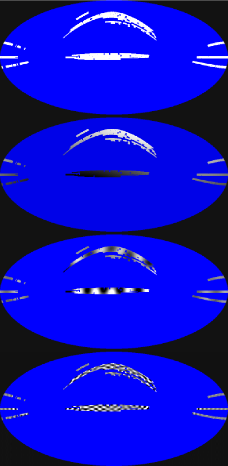
Figure 8.— A sample of four angular pseudo-KL (PKL) modes are shown in Hammer-Aitoff projection in equatorial coordinates, with grey representing zero weight, and lighter/darker shades indicating positive/negative weight, respectively. Uniform blue/grey areas are outside the observed region. From top to bottom, they are angular modes 1 (the mean mode), 3, 35 and 286, and are seen to probe progressively smaller angular scales.

3.4. Step 2: Pseudo-KL pixelization

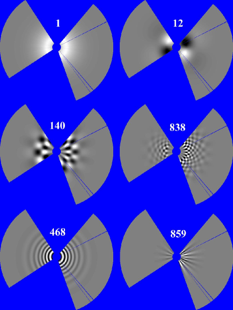
Figure 9.— A sample of six pseudo-KL modes are shown in the equatorial plane. Grey represents zero weight, and lighter/darker shades indicate positive/negative weight, respectively. Uniform blue/grey areas are outside the volume used. The bottom row gives examples of special modes, showing a purely radial mode (left) and a purely angular mode (right).

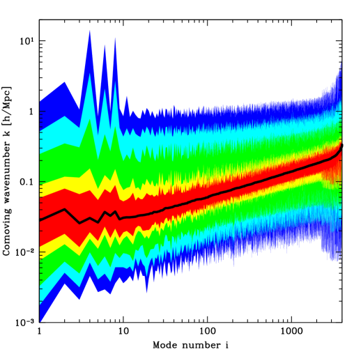
Figure 10.— Relation between mode number $i$ and physical scale $k$. The variance $\langle x_{i}^{2}\rangle$ gets non-negative contributions from all $k$ as per equation (8). $50\%$ of the contribution comes from below the solid black curve, which we can interpret as the median $k$-value probed by the $i^{th}$ mode. The shaded regions show percentiles of the contribution: from outside in, they show the k-ranges giving $99.98\%$, $99.8\%$, $98\%$, $80\%$ and $60\%$ of the contribution, respectively. Apart from the first 8 special modes, the modes are ordered by increasing median $k$-value.

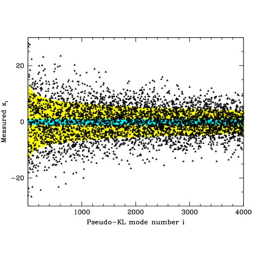
Figure 11.— The triangles show the 4000 elements $x_{i}$ of the data vector ${\bf x}$ (the pseudo-KL expansion coefficients) for the baseline galaxy sample. If there were no clustering in the survey, merely shot noise, they would have unit variance, and about $68\%$ of them would lie within the blue/dark grey band. If our prior power spectrum were correct, then the standard deviation would be larger, as indicated by the shaded yellow/light grey band. To reduce clutter, the modes are (apart from the first 8 special modes), ordered by decreasing signal-to-noise ratio, which corresponds approximately to the ordering by scale in Figure 10.

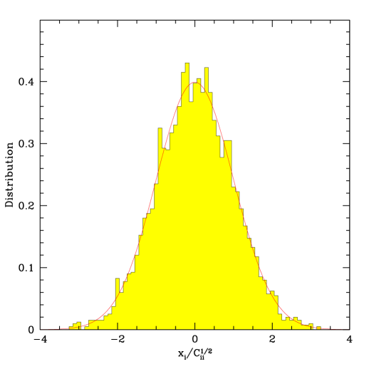
Figure 12.— Gaussianity of fluctuations. The histogram shows the distribution of the 4000 PKL coefficients $x_{i}$ from the previous figure after dividing by their predicted standard deviation ${\bf C}_{ii}^{1/2}$, assuming our prior power spectrum. The histogram has been normalized to have unit area. The solid curve shows a Gaussian of unit variance, zero mean, and unit area.

The raw data consist of three-dimensional vectors ${\bf r}_{\alpha}$, $\alpha=1,...,N_{\rm gal}$, giving the measured positions of each galaxy in redshift space, with the number of galaxies $N_{\rm gal}$ given in Table 1 for each sample. As in Tegmark et al. (1998), we expand the observed three-dimensional density field in a basis of ${N_{x}}$ noise-orthonormal functions $\psi_{i}$, $i=1,...,{N_{x}}$,

$$x_{i}\equiv\int_{V}{n({\bf r})\over{\bar{n}}({\bf r})}\psi_{i}({\bf r})d^{3}r$$ (2)

and work with the ${N_{x}}$-dimensional data vector ${\bf x}$ of expansion coefficients instead of the $3\times N_{\rm gal}$ numbers ${\bf r}_{\alpha}$. Here, ${\bar{n}}$ is the three-dimensional selection function described in Section 2, i.e., ${\bar{n}}({\bf r})dV$ is the expected (not the observed) number of galaxies in a volume $dV$ about ${\bf r}$ in the absence of clustering, and the integration is carried out over the volume $V$ of the sample where the selection function ${\bar{n}}({\bf r})$ is nonzero. We will frequently refer to the functions $\psi_{i}$ as “modes”. As we will see below, these modes play a role quite analogous to pixels in CMB maps, with the variance of $x_{i}$ depending linearly on the power spectrum that we wish to measure.

Galaxies are (from a cosmological perspective) delta-functions in space, so the integral in equation (2) reduces to a discrete sum over galaxies. We do not rebin the galaxies spatially, which would artificially degrade the resolution. It is convenient to isolate the mean density into a single mode $\psi_{1}({\bf r})={\bar{n}}({\bf r})$, with amplitude

$$x_{1}=\int n({\bf r})d^{3}r=N_{\rm gal},$$ (3)

and to arrange for all other modes to have zero mean

$$\langle x_{i}\rangle=\int\psi_{i}({\bf r})d^{3}r=0\quad(i\neq 1).$$ (4)

The covariance matrix of the vector ${\bf x}$ of amplitudes is a sum of noise and signal terms

$$\langle\Delta{\bf x}\Delta{\bf x}^{t}\rangle={\bf C}\equiv{\bf N}+{\bf S}.$$ (5)

where the shot noise covariance matrix is given by

$${\bf N}_{ij}=\int_{V}{\psi_{i}({\bf r})\psi_{j}({\bf r})\over{\bar{n}}({\bf r})}d^{3}r$$ (6)

and the signal covariance matrix is

$${\bf S}_{ij}=\int\widehat{\psi}_{i}({\bf k})\widehat{\psi}_{j}({\bf k})^{*}P_{\rm gg}(k){d^{3}k\over(2\pi)^{3}}$$ (7)

in the absence of redshift-space distortions (which will be included in Section 3.5). Here hats denote Fourier transforms and the star denotes complex conjugation. $P_{\rm gg}(k)$ is the (real-space) galaxy power spectrum, which for a random field of density fluctuations $\delta({\bf r})$ is defined by $\langle\widehat{\delta}({\bf k})\widehat{\delta}({\bf k}^{\prime})^{*}\rangle=(2\pi)^{3}\delta_{\rm Dirac}({\bf k}-{\bf k}^{\prime})P_{\rm gg}(k)$. We take the functions $\psi_{i}$ to have units of inverse volume, so ${\bf x}$, ${\bf N}$, ${\bf S}$ and $\widehat{\psi}_{i}$ are all dimensionless.

Our method requires computing the signal covariance matrix ${\bf S}$, both to calculate power spectrum error bars and to find the power spectrum estimator that minimizes them. Equation (7) shows that this requires assuming a power spectrum $P_{\rm gg}(k)$. For this spectrum, which we refer to as our prior, we use a simple two-parameter fit as described in Section B.4.1, whose parameters are determined from our measurements by iterating the entire analysis.

As our functions $\psi_{i}({\bf r})$, we use the pseudo-Karhunen-Loève (PKL) eigenmodes defined in Hamilton, Tegmark & Padmanabhan (2000; hereafter “HTP00”) and Tegmark, Hamilton & Xu (2002; hereafter “THX02”). The construction of these PKL modes $\psi_{i}({\bf r})$ explicitly uses the three-dimensional selection function ${\bar{n}}({\bf r})$, but is model-independent since it does not depend on the power spectrum.

To provide an intuitive feel for the nature of these modes, a sample is plotted in Figure 8 and Figure 9. We use these modes because they have the following desirable properties:

1. They form a complete set of basis functions probing successively smaller scales, so that a finite number of them (we use the first 4000, for the reasons given in Section B.4.2) allow essentially all information about the density field on large scales to be distilled into the vector ${\bf x}$.

2. They are orthonormal with respect to the shot noise, i.e., such that equation (6) gives ${\bf N}={\bf I}$, the identity matrix. The construction of the modes thus depends explicitly on the survey geometry as specified by ${\bar{n}}({\bf r})$, and $\psi_{i}({\bf r})=0$ in regions of space where ${\bar{n}}({\bf r})=0$.

3. They allow the covariance matrix ${\bf S}$ to be fairly rapidly computed.

4. They are the product of an angular and a radial part, i.e., take the separable form $\psi_{i}({\bf r})=\psi_{i}(\widehat{\bf r})\psi_{i}(r)$, which accelerates numerical computations and helps isolate radial and angular systematic problems.

5. A range of potential sources of systematic problems are isolated into special modes that are orthogonal to all other modes. This means that we can test for the presence of such problems by looking for excess power in these modes, and immunize against their effects by discarding these modes.

We have four types of such special modes:

1. The very first mode is the mean density, $\psi_{1}({\bf r})={\bar{n}}({\bf r})$. The mean mode is used in determining the maximum likelihood normalization of the selection function, but is then discarded from the analysis, since it is impossible to measure the fluctuation of the mean mode. The idea of solving the so-called integral constraint problem by making all modes orthogonal to the mean (Eq. 4) goes back to Fisher et al. (1993).

2. Modes 2-8 are associated with the motion of the Local Group through the Cosmic Microwave Background at 622 km/s towards (B1950 FK4) RA = $162^{\circ}$, Dec = $-27^{\circ}$ (Lineweaver et al. 1996; Courteau & van den Bergh 1999). To first order, these modes are the only modes affected by mis-estimates of the motion of the Local Group.

3. Purely radial modes (for example mode 468 in Figure 9) are to first order the only ones affected by mis-estimates of the radial selection function ${\bar{n}}(r)$.

4. Purely angular modes (for example mode 859 in Figure 9) are to first order the only ones affected by mis-estimates of the angular selection function ${\bar{n}}(\widehat{\bf r})$, as may result from inadequate corrections for, e.g., extinction, the variable magnitude limit, the variable magnitude completeness or photometric zero-point offsets.

The computation of the modes in practice is described in detail in THX02 and in even more detail in Hamilton & Tegmark (2003).

The pixelized data vector ${\bf x}$ is shown in Figure 11. This data compression step has thus distilled the large-scale information about the galaxy density field from $3\times N_{\rm gal}=429{,}942$ galaxy coordinates into 4000 PKL-coefficients. The order of these coefficients is one of decreasing scale (increasing $k$) as is shown in Figure 10. If there were no cosmological density fluctuations in the survey, merely Poisson fluctuations, the PKL-coefficients $x_{i}$ would be uncorrelated with unit variance (since ${\bf N}={\bf I}$), so about $68\%$ of them would be expected to lie within the blue/dark grey band. Figure 11 shows that the fluctuations are considerably larger than Poisson, especially for the largest-scale modes (to the left), demonstrating the obvious fact that cosmological density fluctuations are present, as expected.

3.5. What we wish to measure: three power spectra, not one

Following HTP00 and THX02, we will measure three separate power spectra, whose ratios encode information about clustering anisotropy due to redshift space distortions. Let us now give their definition and some intuition for how to interpret them.

On large scales where redshift space distortions can be treated in the linear approximation (Kaiser 1987), the signal covariance matrix ${\bf S}$ in equation (5) can be generalized from equation (7) and written in the form

$${\bf S}=\int_{0}^{\infty}\left[{\bf P}_{\rm gg}(k)P_{\rm gg}(k)+{\bf P}_{\rm gv}(k)P_{\rm gv}(k)+{\bf P}_{\rm vv}(k)P_{\rm vv}(k)\right]{k^{2}dk\over(2\pi)^{3}},$$ (8)

where $P_{\rm gg}(k)$, $P_{\rm gv}(k)$ and $P_{\rm vv}(k)$ are three power spectra defined in real space (as opposed to redshift space) and ${\bf P}_{\rm gg}(k)$, ${\bf P}_{\rm gv}(k)$ and ${\bf P}_{\rm vv}(k)$ are known dimensionless matrix-valued functions. We will refer to these three power spectra as the galaxy-galaxy power, the galaxy-velocity power and the velocity-velocity power, respectively, or $gg$, $gv$ and $vv$ for short. Specifically, $P_{\rm gg}(k)$ is the real-space galaxy power spectrum, $P_{\rm vv}(k)$ is the velocity power spectrum and $P_{\rm gv}(k)$ is the cross-power between galaxies and velocity. More rigorously, ‘velocity’ here refers to minus the velocity divergence $\nabla\cdot{\bf v}$, which in linear theory is related to the mass (not galaxy) overdensity $\delta$ by $f\delta+\nabla\cdot{\bf v}=0$, where $\nabla$ denotes the comoving gradient in velocity units. Here $f\approx\Omega_{\rm m}^{0.6}$ is the dimensionless growth rate for linear density perturbations (see Hamilton 2001). The three matrix-valued functions are determined directly from the modes $\psi_{i}$, i.e., by geometry alone:

$${({\bf P}_{\rm gg})}_{ij} = \int\widehat{\psi}_{i}({\bf k})\widehat{\psi}_{j}({\bf k})^{*}d\Omega_{k},$$ (9)

$${({\bf P}_{\rm gv})}_{ij} = \int[\widehat{\psi}_{i}({\bf k})\widehat{\zeta}_{j}({\bf k})^{*}+\widehat{\zeta}_{i}({\bf k})\widehat{\psi}_{j}({\bf k})^{*}]d\Omega_{k},$$ (10)

$${({\bf P}_{\rm vv})}_{ij} = \int\widehat{\zeta}_{i}({\bf k})\widehat{\zeta}_{j}({\bf k})^{*}d\Omega_{k},$$ (11)

in which the velocity mode $\widehat{\zeta}_{i}({\bf k})$ is related to the position mode $\widehat{\psi}_{i}({\bf k})$ by (Fisher, Scharf & Lahav 1994; Heavens & Taylor 1995; Hamilton 1998 eq. 8.13)

$$\zeta_{i}={\bf M}^{\dagger}\psi_{i}$$ (12)

where ${\bf M}^{\dagger}$ is the Hermitian conjugate of the velocity part of the linear redshift distortion operator. In the small-angle, or distant observer, approximation, the operator ${\bf M}$ takes the familiar Kaiser (1987) form, a diagonal operator in Fourier space

$${\bf M}\approx\mu_{\bf k}^{2}$$ (13)

where $\mu_{\bf k}\equiv\widehat{\bf k}\cdot{\bf z}$ is the cosine of the angle between the wavevector ${\bf k}$ and the line of sight ${\bf z}$. Here however we do not assume the small-angle approximation, but rather take into account the full radial nature of redshift distortions. Radial redshift distortions destroy translation invariance, so that the radial redshift distortion operator is no longer diagonal in Fourier space, as it is in the small-angle approximation; indeed, the radial redshift distortion operator takes a rather complicated form in Fourier space (Hamilton 1998, eq. 4.37). The radial redshift distortion operator takes a simpler form in real space, where ${\bf M}$, expressed in the frame of the Local Group, can be written as the integro-differential operator (Hamilton 1998 eq. 4.46)

$${\bf M}=\left[{\partial^{2}\over\partial r^{2}}+{\alpha({\bf r})\widehat{\bf r}\over r}\,.\left({\partial\over\partial{\bf r}}-\left.{\partial\over\partial{\bf r}}\right|_{{\bf r}=0}\right)\right]\nabla^{-2}$$ (14)

with $\alpha({\bf r})$ the logarithmic derivative of $r^{2}$ times the selection function ${\bar{n}}({\bf r})$,

$$\alpha({\bf r})\equiv{\partial\ln[r^{2}{\bar{n}}({\bf r})]\over\partial\ln r}.$$ (15)

The $\left.\partial/\partial{\bf r}\right|_{{\bf r}=0}$ term inside parentheses in eq. (14), which subtracts from the first term $\partial/\partial{\bf r}$ its value at the position ${\bf r}=0$ of the Local Group, is the term that arises from the motion of the Local Group. The Hermitian conjugate ${\bf M}^{\dagger}$ which enters equation (12) for the velocity mode $\zeta_{i}$ can be written (Hamilton 1998 eq. 4.50)

$${\bf M}^{\dagger}=\nabla^{-2}r^{-2}{\partial\over\partial r}\left({\partial\over\partial r}-{\alpha({\bf r})\over r}\right)r^{2}-{\widehat{\bf r}\over r^{2}}.\left.{\partial\over\partial{\bf r}}\right|_{{\bf r}=0}\nabla^{-2}\alpha({\bf r})r$$ (16)

in which the last term is again the term arising from the motion of the Local Group.

Although the definition of these three power spectra assumes that redshift distortions conform to the linear Kaiser model, they measure useful information from the data even if the linear model fails. In the small-angle (distant observer) approximation, they reduce to simple linear combinations of the monopole, quadrupole and hexadecapole power spectra in redshift space (Cole, Fisher & Weinberg 1994; Hamilton 1998):

034−15800358)​(Ps0(k)Ps2(k)Ps4(k)).fragmentsPgg(k)fragmentsPgv(k)fragmentsPvv(k)fragments 034fragments15800358fragmentsPs0(k)fragmentsPs2(k)fragmentsPs4(k)\left(\hskip-5.69054pt\begin{tabular}[]{c}$P_{\rm gg}(k)$\\[4.0pt] $P_{\rm gv}(k)$\\[4.0pt] $P_{\rm vv}(k)$\end{tabular}\hskip-5.69054pt\right)=\left(\begin{tabular}[]{ccc}$1$&$-{1\over 2}$&${3\over 8}$\\[4.0pt] $0$&${3\over 4}$&$-{15\over 8}$\\[4.0pt] $0$&$0$&${35\over 8}$\end{tabular}\right)\left(\hskip-5.69054pt\begin{tabular}[]{c}$P^{\rm s}_{0}(k)$\\[4.0pt] $P^{\rm s}_{2}(k)$\\[4.0pt] $P^{\rm s}_{4}(k)$\end{tabular}\hskip-5.69054pt\right).

1-12381-1238 (17)

Whereas the vector on the right hand side is closer to the measurements (and also more familiar in the literature), the vector on the left hand side is closer to the physics of linear redshift distortions. Indeed, inverting equation (17),

$$\left(\hskip-5.69054pt\begin{tabular}[]{c}$P^{\rm s}_{0}(k)$\\[4.0pt] $P^{\rm s}_{2}(k)$\\[4.0pt] $P^{\rm s}_{4}(k)$\end{tabular}\hskip-5.69054pt\right)=\left(\begin{tabular}[]{ccc}$1$&${2\over 3}$&${1\over 5}$\\[4.0pt] $0$&${4\over 3}$&${4\over 7}$\\[4.0pt] $0$&$0$&${8\over 35}$\end{tabular}\right)\left(\hskip-5.69054pt\begin{tabular}[]{c}$P_{\rm gg}(k)$\\[4.0pt] $P_{\rm gv}(k)$\\[4.0pt] $P_{\rm vv}(k)$\end{tabular}\hskip-5.69054pt\right),$$ (18)

we see that we can use this last equation as an improved definition of monopole, quadrupole and hexadecapole, remaining valid even in the regime where the small-angle approximation fails. For the reader more used to thinking in terms of the multipole formalism, the bottom line is that our main measurement $P_{\rm gg}(k)$ is basically the monopole power minus half the quadrupole power plus three eights of the hexadecapole power, as per equation (17).

Because redshift distortions displace galaxies only along the line of sight, the transverse, or angular, power spectrum is completely unaffected by redshift distortions, a point emphasized by Hamilton & Tegmark (2002). In the small-angle approximation, the galaxy-galaxy power spectrum equals the redshift space power spectrum in the transverse direction,

$$P_{\rm gg}(k)=P^{\rm s}(\mu_{\bf k}=0)=\sum_{\l~{}\rm{even}}{(-1)^{\l/2}(\l-1)!!\over\l!!}P^{\rm s}_{\l}(k),$$ (19)

which is true in all circumstances, linear or nonlinear, regardless of the character of redshift distortions. The coefficients of the expansion (19) are the values of Legendre polynomials ${\cal P}_{\l}(\mu_{\bf k})$ in the transverse direction $\mu_{\bf k}=0$. The first few terms of the expansion (19) are

$$P_{\rm gg}(k)=P^{\rm s}_{0}(k)-\frac{1}{2}P^{\rm s}_{2}(k)+\frac{3}{8}P^{\rm s}_{4}(k)-\frac{15}{48}P^{\rm s}_{6}(k)+\ldots,$$ (20)

which shows that our linear estimate of $P_{\rm gg}(k)$ is effectively the expansion (19) truncated at the $\l=4$ harmonic, as predicted by linear theory (Kaiser 1987). We expect on general grounds that the linear estimate of $P_{\rm gg}(k)$ will underestimate the true galaxy-galaxy power spectrum at nonlinear scales (Hamilton & Tegmark 2002), although this underestimate should be mitigated by FOG compression.

In Section 4, we will demonstrate with Monte Carlo simulations that $P_{\rm gg}$ faithfully recovers the true real-space galaxy power spectrum on large scales, and we will quantify what constitutes “large”, finding accurate recovery on substantially smaller scales that those where the Kaiser approximation is valid.

A wide range of approximations for $P_{\rm gv}$ and $P_{\rm vv}$ have been introduced in the literature. Using our notation, the Kaiser (1987) approximation becomes simply

$$P_{\rm gv}(k) = \beta(k)r(k)P_{\rm gg}(k),$$ (21)

$$P_{\rm vv}(k) = \beta(k)^{2}P_{\rm gg}(k),$$ (22)

where $\beta(k)\equiv f/b(k)$, $b(k)$ is the bias factor, $r(k)$ is the dimensionless correlation coefficient between the galaxy and matter density (Dekel & Lahav 1999; Pen 1998; Tegmark & Peebles 1998) and $f\approx\Omega_{\rm m}^{0.6}$ was defined above. Since both $b$ and $r$ can in principle depend on scale, we have two unknown functions $\beta(k)$ and $r(k)$ that can in principle be determined uniquely from the two measured ratios $P_{\rm gv}(k)/P_{\rm gg}(k)$ and $P_{\rm vv}(k)/P_{\rm gg}(k)$ in the Kaiser approximation. Further popular approximations in the literature are that both $b$ and $r$ are constant, and most workers also assume $r=1$ despite some observational (Tegmark & Bromley 1999; Blanton 2000) and simulational (Blanton et al. 1999; Cen & Ostriker 2000; Somerville et al. 2001) evidence that $r$ may be of the order of 0.9 for some galaxies.

We will not make any of these approximations in our basic data analysis, simply reporting measurements of $P_{\rm gg}(k)$, $P_{\rm gv}(k)$ and $P_{\rm vv}(k)$ from the SDSS data. In Section 4 we use the approximation that $\l>4$ anisotropies are negligible, assessing its accuracy with Monte Carlo simulations and tunable finger-of-god compression, but the reader wishing to avoid approximations can simply fit better simulations directly to our three measured curves. Specifically, using an axis of a periodic cube as the line-of-sight direction, so that the distant observer approximation holds perfectly, one can compute the monopole, quadrupole, and hexadecapole components of the redshift-space power spectrum and transform them to $P_{\rm gg}$, $P_{\rm gv}$, and $P_{\rm vv}$ via equation (17).

3.6. Step 3: Power spectrum estimation

All our information about the SDSS density field is encoded in the 4000-dimensional vector ${\bf x}$ plotted in Figure 11, and equation (8) shows that the covariance matrix of ${\bf x}$ depends linearly on the three power spectra that we want to measure. We wish to invert equations (5) and (8) to estimate the power spectra from the data vector. This problem is mathematically equivalent to that of measuring the power spectrum from a CMB map, and can be solved optimally with so-called quadratic estimators (Tegmark 1997b; Bond et al. 2000). We describe our analysis method in full detail in Appendix B. However, since it is important for the interpretation, let us briefly review here how the measurements are computed from the input data ${\bf x}$.

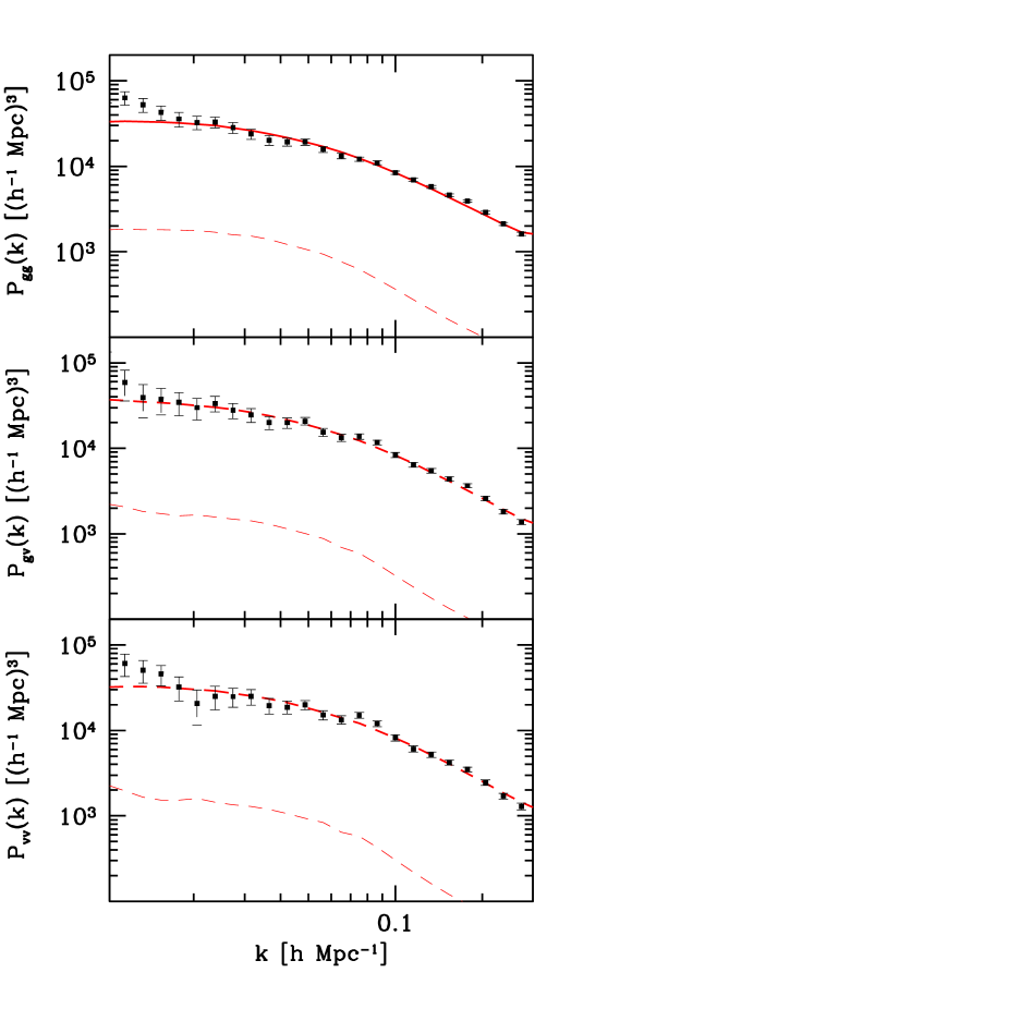
Figure 13.— The minimum-variance quadratic estimators $\widehat{p}_{i}$ nominally measuring the galaxy-galaxy power spectrum (top), the galaxy-velocity power spectrum (middle) and the velocity-velocity power spectrum (bottom) for the baseline galaxy sample. They cannot be directly interpreted as power spectrum measurements, since each point probes a linear combination of all three power spectra over a broad range of scales, typically centered at a $k$-value different than the nominal $k$ where it is plotted. Moreover, nearby points are strongly correlated, causing this plot to overrepresent the amount of information present in the data. The solid curves show the window-convolved prior power spectrum ${\bf W}{\bf p}$, and the dashed curve shows the shot noise contribution subtracted out.

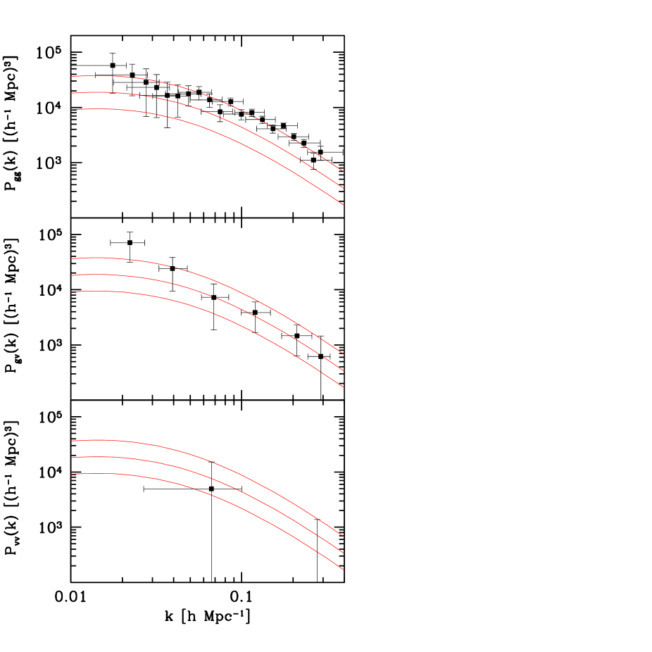
Figure 14.— Decorrelated and disentangled measurements of the galaxy-galaxy power spectrum (top), the galaxy-velocity power spectrum (middle) and the velocity-velocity power spectrum (bottom) for the baseline galaxy sample. Each point is plotted at the $k$-value that is the median of its window function, and the horizontal bars range from the 20th to the 80th percentile of the window function. The values of $P_{\rm gg}(k)$ are given in Table 3. From top to bottom, the three curves shows our prior for $P_{\rm gg}(k)$, $P_{\rm gv}(k)$ and $P_{\rm vv}(k)$. Note that most of the information in the survey is in the galaxy-galaxy spectrum. Band-power measurements with very low information content have been binned into fewer (still uncorrelated) bands. All these measurements are for our baseline FOG compression threshold of 200. Unlike Figure 13, these points are uncorrelated (affecting all three panels) and the leakage between $gg$, $gv$ and $vv$ has been removed (affecting mostly the lower panels), giving much larger (and easier to interpret) error bars.

We parameterize our three power spectra by their amplitudes in 97 separate logarithmically spaced $k$-bands as detailed in Appendix B, so our goal is to measure $3\times 97=291$ band powers $p_{i}$, $i=1,...,291$. Quadratic estimators $\widehat{p}_{i}$ are simply quadratic functions of the data vector ${\bf x}$, and the most general unbiased case can be written as

$$\widehat{p}_{i}\equiv{\bf x}^{t}{\bf Q}_{i}{\bf x}-\hbox{tr}\,[{\bf N}{\bf Q}_{i}],$$ (23)

for some symmetric $N\times N$-dimensional matrices ${\bf Q}_{i}$; the second term merely subtracts off the expected contribution from the shot noise.

The basic idea behind quadratic estimators is that each matrix ${\bf Q}_{i}$ can be chosen to effectively Fourier transform the density field, square the Fourier modes in the $i^{th}$ power spectrum band and average the results together, thereby probing the power spectrum on that scale. Grouping the parameters $p_{i}$ and the estimators $\widehat{p}_{i}$ into vectors denoted ${\bf p}$ and $\widehat{\bf p}$, the expectation value and covariance of the measurements is given by

$$\langle\widehat{\bf p}\rangle = {\bf W}{\bf p},$$ (24)

$${\rm cov}(\widehat{\bf p}) \equiv \langle\widehat{\bf p}\widehat{\bf p}^{t}\rangle-\langle\widehat{\bf p}\rangle\langle\widehat{\bf p}\rangle^{t}=\SS,$$ (25)

where the matrices ${\bf W}$ and $\SS$ can be computed from the ${\bf Q}_{i}$-matrices and the geometry alone via equations (B10) and (B11) in Appendix B.

As detailed in Appendix B, there are several attractive choices of ${\bf Q}$-matrices, each giving different desirable properties to the matrices ${\bf W}$ and $\SS$. Figure 13 shows the power spectrum measurements $\widehat{\bf p}$ for the baseline galaxy sample using the choice of ${\bf Q}_{i}$ that gives the smallest error bars, and Figure 14 shows them using a better choice described below.

Although Figure 13 looks impressive, it fails to convey two important complications. The first is that the error bars are strongly correlated between neighboring bands, i.e., the covariance matrix $\SS$ is far from diagonal. The second complication involves the matrix ${\bf W}$, known as the window matrix. The ${\bf Q}$-matrices are normalized so that each row of the window matrix sums to unity. Equation (24) shows that this normalization enables us to interpret each band power measurement $\widehat{p}_{i}$ as a weighted average of the true power spectrum $p_{j}$, the elements of the $i^{th}$ row of ${\bf W}$ giving the weights (the so-called window function). In short, the window functions connect our measurements $\widehat{\bf p}$ to the underlying power spectrum parameters ${\bf p}$. The windows are plotted in Figure 15, and we see that they are complicated in two different ways, making Figure 13 hard to interpret:

1. Smearing: They have a non-zero width $\Delta k$, so that our estimate of the power on some scale $k$ is really the weighted average of the power over a range of scales around $k$. In other words, Figure 13 shows a measurement of the true power spectrum that has been smoothed, convolved with rather broad window functions.

2. Leakage: They mix the $gg$, $gv$ and $vv$ power spectra, so that a nominal estimate of $gv$, say, is really a weighted average of $gg$, $gv$ and $vv$ power. This is why the signal-to-noise ratio of $gv$ and $vv$ appear so high in Figure 13.

As described in Appendix B, both the correlation problem and the smearing problem can be tackled in one fell swoop with a better choice of quadratic estimators that give uncorrelated error bars and narrower window functions, shown in Figure 16. This choice makes the covariance matrix $\SS$ for the measured vector $\widehat{\bf p}$ diagonal (combining shot noise and sample variance errors), so it is completely characterized by its diagonal elements, given by the error bars in Table 2 and Figure 14. A clearer and less cluttered view of a sample window function for this uncorrelated case is given in Figure 18 (top left panel). We see that such a window is almost never negative, and tends to be sharply peaked around the $k$-value that it is designed to probe.

Let us now turn to the remaining problem: leakage. The leakage results from a combination of two effects: difficulties in separating the monopole, quadrupole and hexadecapole power given the complicated survey geometry, and the mixing of these three multipoles given by equation (17). Figures 15, 16 and 17 show the $i^{th}$ window function (the $i^{th}$ row of the ${\bf W}$-matrix) as three curves plotted in the top, middle and bottom panels, giving the sensitivity of the estimator $\widehat{p}_{i}$ to $gg$, $gv$ and $vv$ power, respectively. If there were no leakage, then all curves in the six off-diagonal panels in these figures would be identically zero. This is not the case, but the area under the curves is much reduced in the off-diagonal panels, as is shown by comparing the left-most and middle panels of Figure 19. Switching to uncorrelated quadratic estimators causes a substantial leakage reduction as a side benefit, but that leakage is still non-negligible: for instance, an estimate of the $gg$ power is seen to give about 15% weight to $P_{\rm gv}$ and about 2% weight to $P_{\rm vv}$, with these percentages depending only weakly on $k$.

As detailed in Appendix B, we can eliminate the leakage problem and measure one power spectrum, say $P_{\rm gg}(k)$, without any assumptions about the other two by effectively marginalizing over their amplitudes separately for each $k$-band. This procedure is equivalent to yet another choice of the ${\bf Q}$-matrices, which we refer to as disentangled. As seen in Figure 17 and the right panels of Figure 19, it eliminates leakage completely in the sense that all unwanted (off-diagonal) window functions have zero area. The basic idea of the disentanglement procedure is illustrated in Figure 18: since the $gg$, $gv$ and $vv$ components of the window function have very similar shape, differing essentially only in amplitude, it is possible to form linear combinations of them that for all practical purposes vanish. In forming these linear combinations, we do introduce statistical correlations between $P_{\rm gg}(k)$, $P_{\rm gv}(k)$ and $P_{\rm vv}(k)$ at a given value of $k$; the values at different values of $k$ remain uncorrelated.

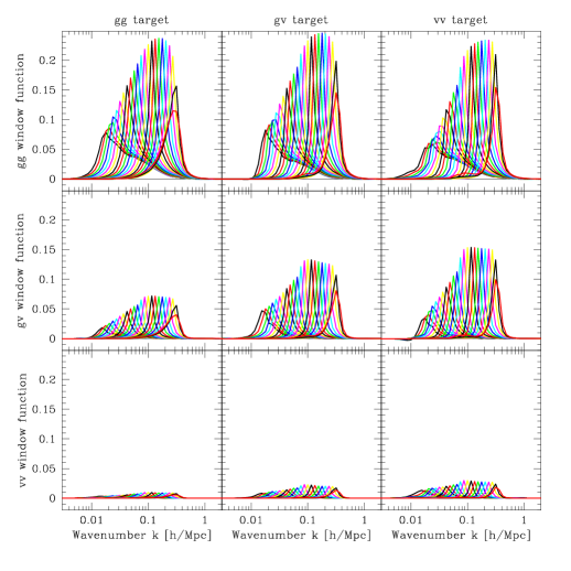
Figure 15.— Using the correlated minimum-variance estimators, the window functions are shown for those $k$-bands with non-negligible information content. The $i^{th}$ row of ${\bf W}$ typically peaks at the $i^{th}$ band, the scale $k$ that the band power estimator $\widehat{p}_{i}$ was designed to probe. The three rows correspond to the estimators of $gg$, $gv$ and $vv$ power and the three columns to their sensitivity to $gg$, $gv$ and $vv$ power. For example, the window function of the quadratic estimator targeting $P_{\rm gv}(k)$ at $k=0.1h/$Mpc is given by the three curves in the middle column peaking at $k=0.1h/$Mpc (top, middle and bottom panels), and the normalization is such that sum of the areas under these three curves is unity.

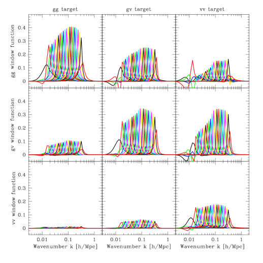
Figure 16.— Same as Figure 15, but using decorrelated estimators (before disentanglement). Comparison with Figure 15 shows that decorrelation makes all windows substantially narrower.

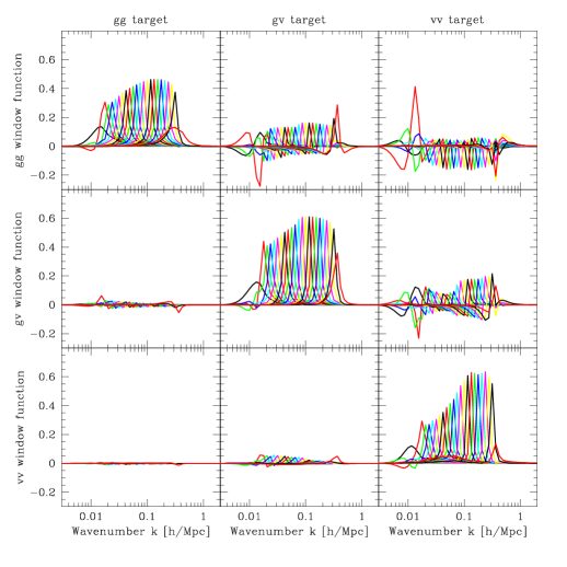
Figure 17.— Same as Figure 16, but decorrelated and disentangled estimators. Comparison with Figure 16 shows that disentanglement gives curves in the off-diagonal panels a vanishing average, and almost completely eliminates leakage of $gv$ and $vv$ power into estimators of $gg$ power (two bottom panels in left column).

Figure 18.— The window function for our measurement of the 49th band of the galaxy-galaxy power is shown before (left) and after (right) disentanglement. Whereas unwanted leakage of $gv$ and $vv$ power is present initially, these unwanted window functions both average to zero afterward. The success of this method hinges on the fact that since the three initial functions (left) have similar shape, it is possible to take linear combinations of them that almost vanish (right). This procedure is repeated separately for each $k$.

In summary, we have measured the three power spectra $P_{\rm gg}(k)$, $P_{\rm gv}(k)$ and $P_{\rm vv}(k)$, obtaining the results shown in Figure 14. These basic measurements are given in Table 2 and are available at
http://www.hep.upenn.edu/$\sim$max/sdss.html together with their window matrix and likelihood calculation software, incorporating the bias correction described in Section 5. The measurements make no assumptions whatsoever about redshift-space distortions, and the issue of whether the density fluctuations are Gaussian affects only the error bars, not the measurements themselves.

In the next section, we will model the effect of redshift distortions and make what we argue is a more accurate estimate of $P_{\rm gg}(k)$. However, the conservative reader trusting only her/his own modeling can in principle stop right here and fit simulations directly to our measurements from Figure 14, which are given in Table 2.

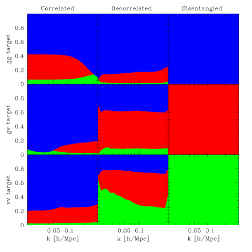
Figure 19.— The leakage is shown for the correlated (left column), decorrelated (middle column) and disentangled (right column) methods. From top to bottom within each box, the three bands (blue/dark grey, red/grey and green/light grey) show the relative contributions from $gg$, $gv$ and $vv$ power, respectively. From top to bottom, the three rows are for estimators are for $gg$, $gv$ and $vv$ power, respectively.

Table 2 – The real-space power spectrum $P_{\rm gg}(k)$ (top), $P_{\rm gv}(k)$ (middle) and $P_{\rm vv}(k)$ (bottom) measured with the disentanglement method. The units of the power are $(h^{-1}{\rm Mpc})^{3}$. $\Delta P$ is the $1\sigma$ error. These values have been corrected for luminosity-dependent bias by dividing by the square of the last column, and thus refer to the clustering of $L_{*}$ galaxies. The $k$-column gives the median of the window function and its $20^{th}$ and $80^{th}$ percentiles; the exact window functions from http://www.hep.upenn.edu/$\sim$max/sdss.html. should be used for any quantitative analysis. The $P_{\rm gg}$ errors are uncorrelated with one another, but are correlated with the $P_{\rm gv}$ and $P_{\rm vv}$ errors. We recommend using column 2 for basic analysis. Column 3 is without FOG removal (i.e., with threshold $\delta_{c}=\infty$) and is therefore easier to compare against numerical simulations.

$k\>[h/$Mpc]	$P$	$P$ ($\perp$FOG)	$\Delta P$	$b$
$0.018^{+0.008}_{-0.004}$	42098	41081	28850	1.167
$0.023^{+0.009}_{-0.005}$	28260	28924	16394	1.167
$0.028^{+0.010}_{-0.005}$	20880	20508	15849	1.166
$0.032^{+0.010}_{-0.006}$	16903	17097	12079	1.165
$0.037^{+0.011}_{-0.007}$	12178	12119	9004	1.164
$0.042^{+0.012}_{-0.008}$	11887	11996	6944	1.163
$0.049^{+0.013}_{-0.009}$	13098	13094	5188	1.161
$0.056^{+0.014}_{-0.010}$	13996	14003	3847	1.159
$0.065^{+0.015}_{-0.012}$	10273	10333	2847	1.157
$0.075^{+0.017}_{-0.014}$	6296	6366	2130	1.153
$0.086^{+0.019}_{-0.016}$	9653	9687	1594	1.149
$0.100^{+0.021}_{-0.018}$	5763	5814	1205	1.144
$0.115^{+0.024}_{-0.021}$	6229	6273	921	1.139
$0.132^{+0.027}_{-0.025}$	4693	4711	712	1.132
$0.153^{+0.031}_{-0.030}$	3263	3321	554	1.123
$0.176^{+0.035}_{-0.037}$	3778	3811	437	1.114
$0.202^{+0.039}_{-0.045}$	2423	2428	356	1.104
$0.232^{+0.043}_{-0.058}$	1891	1892	312	1.093
$0.264^{+0.043}_{-0.075}$	952	947	304	1.082
$0.290^{+0.047}_{-0.102}$	1340	1385	386	1.074
$0.022^{+0.005}_{-0.005}$	52115	51536	28798	1.167
$0.039^{+0.007}_{-0.009}$	17843	17716	10870	1.164
$0.069^{+0.011}_{-0.015}$	5451	5233	4057	1.155
$0.120^{+0.021}_{-0.028}$	2991	2746	1684	1.137
$0.211^{+0.040}_{-0.047}$	1207	902	684	1.101
$0.291^{+0.047}_{-0.039}$	537	319	720	1.074
$0.067^{+0.040}_{-0.034}$	3700	3583	7712	1.156
$0.278^{+0.128}_{-0.184}$	7	-81	1185	1.078

Table 3 – The real-space power spectrum $P_{\rm gg}(k)$ in units of $(h^{-1}{\rm Mpc})^{3}$ measured with the modeling method. $\Delta P_{\rm gg}$ is the $1\sigma$ error, uncorrelated between bands. These values have been corrected for luminosity-dependent bias by dividing by the square of the last column (see Section 5), and thus refer to the clustering of $L_{*}$ galaxies. The $k$-column gives the median of the window function and its $20^{th}$ and $80^{th}$ percentiles; the exact window functions from http://www.hep.upenn.edu/$\sim$max/sdss.html. should be used for any quantitative analysis.

$k\>[h/$Mpc]	$P_{\rm gg}$	$\Delta P_{\rm gg}$	$b$
$0.016^{+0.006}_{-0.003}$	21573	33320	1.168
$0.018^{+0.006}_{-0.003}$	33255	24573	1.167
$0.021^{+0.007}_{-0.004}$	13846	17712	1.167
$0.024^{+0.007}_{-0.004}$	38361	13320	1.167
$0.028^{+0.008}_{-0.005}$	24143	10047	1.166
$0.032^{+0.008}_{-0.005}$	19709	7414	1.165
$0.037^{+0.009}_{-0.006}$	12596	5486	1.164
$0.043^{+0.010}_{-0.007}$	13559	4078	1.163
$0.049^{+0.011}_{-0.008}$	18311	2974	1.161
$0.057^{+0.012}_{-0.008}$	12081	2140	1.159
$0.065^{+0.013}_{-0.010}$	9217	1580	1.156
$0.075^{+0.015}_{-0.011}$	9751	1128	1.153
$0.087^{+0.017}_{-0.012}$	9530	818	1.149
$0.100^{+0.019}_{-0.014}$	6385	602	1.144
$0.116^{+0.021}_{-0.016}$	5295	447	1.138
$0.134^{+0.024}_{-0.019}$	4630	335	1.131
$0.154^{+0.027}_{-0.022}$	3574	254	1.123
$0.178^{+0.031}_{-0.027}$	3394	195	1.114
$0.205^{+0.036}_{-0.032}$	2298	153	1.103
$0.236^{+0.041}_{-0.039}$	1597	124	1.092
$0.271^{+0.043}_{-0.048}$	1105	107	1.080
$0.306^{+0.042}_{-0.075}$	1013	110	1.069

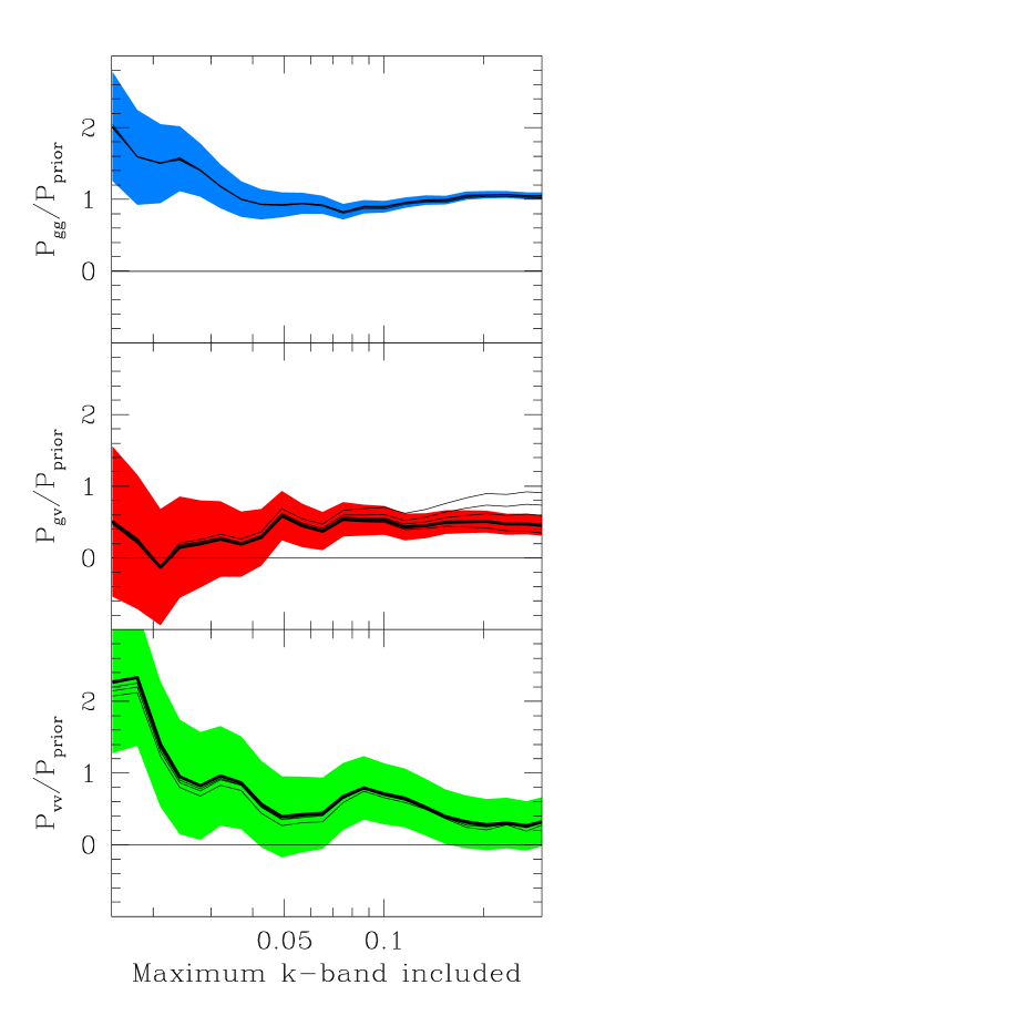
Figure 20.— The blue, red and green bands show the $1\sigma$ allowed ranges for the amplitude of the $gg$, $gv$ and $vv$ power, respectively, relative to the prior $gg$ spectrum, as a function of the maximum wavenumber included in the fit. The sets of five black curves show the best fit values using FOG compression with the five density thresholds $1{+}\delta_{c}=\infty$ (no FOG compression), 200 (our baseline; heavy curve), 100, 50 and 25 (successive curves go higher for $gv$ and lower for $gg$ and $vv$).

4. Accounting for redshift space distortions

So far, we have measured the SDSS galaxy power spectrum and its redshift-space anisotropy, encoded in the three functions $P_{\rm gg}(k)$, $P_{\rm gv}(k)$ and $P_{\rm vv}(k)$. In the present section, we focus on this anisotropy to model, quantify and correct for the effects of redshift-space distortions, producing an estimate of the true real-space galaxy power spectrum, $P_{\rm gg}^{\rm true}(k)$. We will use Monte-Carlo simulations to assess the accuracy of two alternative approaches:

1. Disentanglement approach: perform FOG compression, then simply use $P_{\rm gg}(k)$ from Figure 14 as the estimator of $P_{\rm gg}^{\rm true}(k)$.

2. Modeling approach: perform FOG compression, then make the Kaiser approximation of equations (21) and (22) with the best-fit constant values of $\beta$ and $r$ to eliminate $P_{\rm gv}(k)$ and $P_{\rm vv}(k)$ from the problem, solving for the 97 decorrelated measurements of $P_{\rm gg}^{\rm true}(k)$ (see Appendix B and THX02 for details).

The difference between the two approaches is essentially between marginalizing over the other two power spectra ($P_{\rm gv}(k)$ and $P_{\rm vv}(k)$) and modeling them. Both approaches break down on small scales, so we focus on quantifying their accuracy as a function of $k$. We will see that although the disentanglement approach is more robust to nonlinearities, the modeling approach has the advantage of roughly halving the error bars, corresponding to quadrupling the Fisher information. The gain comes from using rather than discarding measured information about the amplitudes of the $gv$ and $vv$ power spectra. We will argue that the disentanglement method is overly conservative, especially on extremely large scales like $k<0.05h/$Mpc where we need all the statistical power that we can get.

There are two separate sources of statistical bias in our measurement that we will quantify below. The first is that $P_{\rm gg}(k)$ will only equal the true real-space power on scales on which the Kaiser approximation holds, generally underestimating it on smaller scales. The second occurs only in the modeling approach, which produces a biased measurement of $P_{\rm gg}(k)$ if the model parameters $\beta$ and $r$ are incorrect.

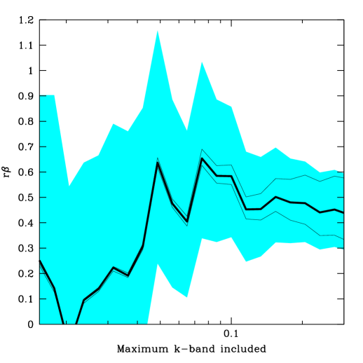
Figure 21.— The blue/grey band shows the $1\sigma$ allowed range for $r\beta$, assuming the shape of the prior $P_{\rm gg}(k)$ but marginalizing over the power spectrum normalization, using FOG compression with our baseline density threshold $1{+}\delta_{c}=200$. From bottom to top, the three curves show the best fit $\beta$ for FOG thresholds $1{+}\delta_{c}=\infty$ (no FOG compression), 200 (our baseline; heavy curve) and 100.

Let us begin our investigation by studying the real data, then turn to Monte Carlo simulations to better understand and quantify the results.

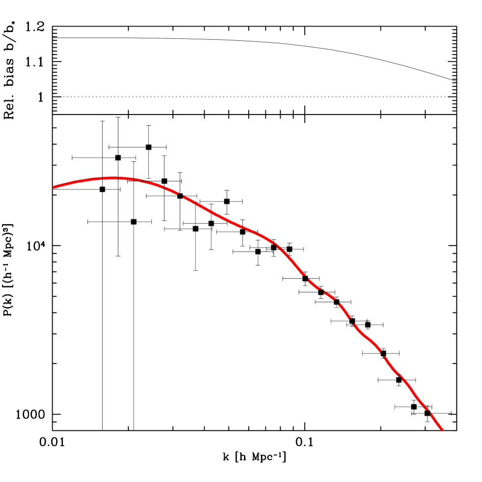
Figure 22.— The decorrelated real-space galaxy-galaxy power spectrum using the modeling method is shown (bottom panel) for the baseline galaxy sample assuming $\beta=0.5$ and $r=1$. As discussed in the text, uncertainty in $\beta$ and $r$ contribute to an overall calibration uncertainty of order $4\%$ which is not included in these error bars. To remove scale-dependent bias caused by luminosity-dependent clustering, the measurements have been divided by the square of the curve in the top panel, which shows the bias relative to $L_{*}$ galaxies. This means that the points in the lower panel can be interpreted as the power spectrum of $L_{*}$ galaxies. The solid curve (bottom) is the best fit linear $\Lambda$CDM model of Section 5.

4.1. Results based on the data

Figure 14 shows that whereas we have precise measurements of $P_{\rm gg}(k)$, we have rather limited information about $P_{\rm gv}(k)$ and close to no information about $P_{\rm vv}(k)$. Figure 20 shows a slightly less noisy rendition of the same information. Here we have taken all three curves to have the shape of the prior power spectrum and plotted their best-fit amplitudes relative to the prior. These fits are performed cumulatively, using all measurements for all wavenumbers $\leq k$. The three bands give the $1\sigma$ allowed ranges for $gg$, $gv$ and $vv$, respectively. It is well-known that as $k$ increases, nonlinearities become more important and start reducing $gv$, eventually driving it negative. This is because the FOG effect has the opposite sign of the linear Kaiser infall, causing less rather than more radial power (or larger rather than smaller radial correlations, for the reader preferring real space over Fourier space). The fact that Figure 20 does not show this effect is therefore a first encouraging indication that nonlinearities have only a minor impact on our results over the range of scales that we consider. Since we have used only 4000 PKL modes, most of the information from scales $k\gg 0.1h/$Mpc is excluded from our analysis (cf., Figure 10). The bands in the figure therefore stop getting thinner for $k\gg 0.1h/$Mpc. In other words, the information contained in our data vector ${\bf x}$ describes only a highly smoothed version of the density field, where nonlinear effects are small.

The five thin lines in Figure 20 correspond to our five FOG compression thresholds, and show several noteworthy things. First of all, changing the FOG threshold is seen to have a strong effect on $gv$ but almost no effect on $gg$ (the quantity that we really care about in this paper), providing another encouraging indication that virialized structures do not pose an unsurmountable problem for us. Second, more aggressive FOG removal is seen to raise the $gv$ amplitude. This is the expected sign of the effect, since it removes (and eventually over-corrects for) the FOG effect which suppresses $gv$. Third, the $gg$ and $gv$ curve pentuplets are seen to diverge as $k$ increases, as nonlinearities become more important. For $gv$, the spread between the baseline threshold $1+\delta_{c}=200$ and the rather extreme neighboring thresholds ($100$ and $\infty$) equals the error bar for $k\sim 0.3h/{\rm Mpc}$, suggesting that nonlinearity-related uncertainties become comparable to statistical uncertainties on this scale when trying to measure the redshift distortion parameter $\beta$. For $gg$, on the other hand, the statistical uncertainties dominate on all scales to which we are sensitive. The optimal FOG compression threshold should be expected to lie somewhere between our options $200$ and $\infty$, since $1{+}\delta_{c}=200$ is the approximate overdensity of a cluster that has just formed, and many FOG systems will have formed earlier and hence have higher overdensities. The other thresholds plotted, i.e., 100, 50, and 25, are thus more extreme and eventually unphysical — we have used and plotted them merely to exaggerate and illustrate the effect of FOG removal more clearly.

Since $vv$ is so noisy, our main constraint on redshift space distortion comes from the ratio of $gv$ to $gg$ power, i.e., on $r\beta=P_{\rm gg}/P_{\rm gv}$. Figure 21 shows our $1-\sigma$ constraints on $r\beta$ as a function of the maximal $k$-band included in a cumulative fit, discarding the $vv$ information to be conservative. The effect of FOG removal is seen to be smaller than the statistical errors for all scales that we consider. Our (loose) constraints agree well with a previous $\beta$-measurement from earlier SDSS data (Zehavi et al. 2002) and also with measurements from the 2dFGRS (Peacock et al. 2001; THX02) assuming that the bias does not differ dramatically between the $r$-band selected SDSS galaxies and $B$-band selected 2dF galaxies. We are unable to break their near degeneracy and place strong constraints on $\beta$ and $r$ separately, but a joint likelihood analysis marginally favors $r\sim 1$.

Our estimate of the real-space galaxy power spectrum from the disentanglement approach is simply the top panel of Figure 14. The corresponding estimate using the model approach is shown in Figure 22; the values are tabulated in Table 3. Here we use $\beta=0.5$ and $r=1$, which provides a good fit to our data. The measurements are also tabulated in Tables 2 and 3. Changing these two parameters within their measurement uncertainty causes an uncertainty of 4% in the overall normalization of the recovered $gg$ power spectrum (which is, of course, degenerate with a 2% change in the galaxy bias). The corresponding window functions are shown in Figure 24; compare with Figure 17.

To indicate how linear the fluctuations are on various scales, Figure 23 shows the square root of the corresponding dimensionless power spectrum, which can be crudely interpreted as the rms fluctuation on that scale. This fluctuation level is seen to drop below 10% on the largest scales, $k\mathrel{\hbox to0.0pt{\lower 3.0pt\hbox{$\mathchar 536\relax$}\hss}\raise 2.0pt\hbox{$\mathchar 318\relax$}}0.02h/$Mpc, with the curve being strikingly different from a power law (more clearly seen in Figure 22). The nonlinearity transition $\Delta\sim 1$ is seen to occur around $k\sim 0.2h$/Mpc, but this is a crude estimate since what matters is of course the fluctuation level of the matter, not of the galaxies, and the two differ by the bias factor. As detailed in Section 7, our $L^{*}$ galaxies have $\sigma_{8}\approx 0.93$, so if $\sigma_{8}\approx 0.8$ for the matter as indicated by many recent CMB, lensing and cluster studies (Lahav et al. 2002; Wang et al. 2002; Bennett et al. 2003), the fluctuations are slightly more linear than Figure 23 indicates.

Figure 23.— The rms density fluctuation amplitude $\Delta(k)^{1/2}$ derived from the modeling method power spectrum of the previous figure, where $\Delta(k)\equiv 4\pi P_{\rm gg}(k)[k/(2\pi)]^{3}$ and $k$ is the effective $k$-value from Table 2.

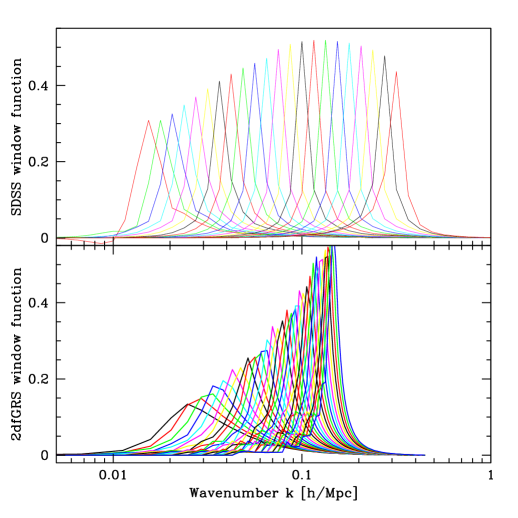
Figure 24.— The SDSS window functions (rows of ${\bf W}$) are shown (top panel) using decorrelated estimators for the modeling method. The $i^{th}$ row of ${\bf W}$ typically peaks at the $i^{th}$ band, the scale $k$ that the band power estimator $\widehat{p}_{i}$ was designed to probe. All curves have been normalized to have the same area, so the highest peaks indicate the scales where the window functions are narrowest. The turnover in the envelope at $k\sim 0.1\,h/{\rm Mpc}$ reflects our running out of information due to omission of modes probing smaller scales. The 32 2dFGRS window functions estimated by Percival et al. (2001) are shown for comparison, plotted with the exact same conventions. They correspond to correlated rather than uncorrelated measurements. Their shapes and widths is seem to agree well with the SDSS windows around $k\sim 0.1h/$Mpc, becoming substantially wider on larger scales; this is a key advantage of our analysis method.

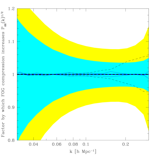
Figure 25.— Effect of finger-of-god (FOG) compression on the measured power spectrum. From bottom to top, the three solid curves show the factor by which the measured fluctuation amplitude $P_{\rm gg}(k)^{1/2}$ is increased by FOG compression with overdensity thresholds $\infty$ (no compression), 200 (our baseline; horizontal line) and 100, respectively, using the disentanglement method. The dashed curves show the same ratios for the modeling method. To place these effects in context, the relative $1\sigma$ measurement errors on the power spectrum amplitude are indicated by the yellow/light grey band for the disentanglement method and by the cyan/grey band for the modeling method.

To quantify the FOG effect on our recovered real-space power spectrum, Figure 25 shows the ratio of the measured power spectrum amplitude to its value with our baseline FOG compression. Just as we saw in Figure 20, nonlinearities become progressively more important toward smaller scales. Quantitatively, the disentanglement method is seen to be almost unaffected by FOG-compression. Over the range $0.1h/{\rm Mpc}<k<0.2h/{\rm Mpc}$ where the error bars are smallest, changing the FOG compression threshold within the rather extreme range $100-\infty$ changes the measured fluctuation amplitude by only about 1%, which should be compared to statistical error bars of 8% or more. The sensitivity of the modeling method to these nonlinear effects is slightly greater: 1% at $k\sim 0.1h/{\rm Mpc}$ and 4% at $k\sim 0.2h/{\rm Mpc}$, again letting the FOG threshold vary across the rather extreme range $100-\infty$.

4.2. Results from Monte Carlo simulations

We need to quantify how accurately what we measure, $P_{\rm gg}(k)$, recovers what we really care about, i.e., the real space matter power spectrum $P(k)$. Nonlinear clustering per se would not bias quadratic estimators of the power spectrum, but how much do non-linearities in the redshift-space distortions affect the results? Figure 25 shows that the sensitivity of the $P_{\rm gg}(k)$-measurement to FOG nonlinearities is around $1\%$ at $k\sim 0.1h/{\rm Mpc}$, i.e., negligible compared to our statistical measurement errors. Although fingers of god are perhaps the most important way in which nonlinear redshift distortions manifest themselves, mildly nonlinear effects on larger scales are also important (Scoccimarro et al. 2001; Scoccimarro 2003). To be prudent, we therefore complement the above-mentioned tests with a Monte Carlo analysis in which the true $P(k)$ is known and we can directly determine how well we recover it.

We use two suites of Monte Carlo simulations as summarized in Table 1. The first consists of 275 simulations constructed with the PThalos code (Scoccimarro & Sheth 2002), covering 1395 square degrees with an angular completeness map corresponding to the northern part of SDSS (sample9, an earlier version of sample11 discussed in Appendix A. In short, this code is a fast approximate method to build non-Gaussian density fields with the halo model. It produces realistic correlation functions and includes non-trivial galaxy biasing by placing galaxies within dark matter halos with a prescribed halo occupation number as a function of halo mass. The second suite of simulated surveys is based on the Hubble volume $\Lambda$CDM $n$-body simulation (Frenk et al. 2000; Evrard et al. 2002). 10 mock surveys were produced by sparse-sampling different parts of the simulation cube to reproduce the three-dimensional selection function ${\bar{n}}({\bf r})$ for SDSS sample8, so although these mock surveys include fully nonlinear gravitational clustering, they have trivial light-to-mass bias with $b=r=1$ (the “galaxies” are simply a random subset of the dark matter particles).

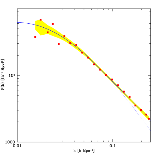
Figure 26.— Squares show the mean power spectrum $P_{\rm gg}(k)$ recovered from 62 PThalos simulations by our analysis pipeline, using the disentanglement method without FOG compression. If these squares faithfully measure the average real-space matter power spectrum of the simulations (solid line), then about 68% of them should lie in the shaded band around this curve, whose width is given by the $1\sigma$ errors computed by our pipeline divided by the square root of the number of simulations. For comparison, the dotted curve shows the linear power spectrum used as input for the simulations.

Figure 26 shows that the average $P_{\rm gg}(k)$ recovered using the methodology described in this paper from the PThalos simulations agrees with the matter $P(k)$ on all relevant scales to within the sensitivity we can test, as expected given the above indications that the effect of nonlinearities on $P_{\rm gg}$ is small. It also confirms that the analysis pipeline produces unbiased results (this was also demonstrated with extensive Monte Carlo simulations in THX02). The mock surveys based on the Hubble Volume simulation give similar agreement, although with larger noise since there are only ten of them.

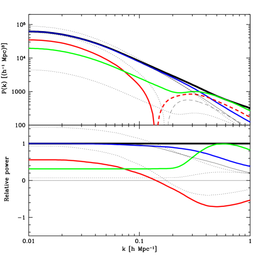
Figure 27.— Power spectra from 275 PThalos mock catalogs, quantifying how accurately our $P_{\rm gg}(k)$ statistic recovers the true power spectrum. The thick black curve in the upper panel shows the real-space power spectrum that we wish to recover, on a logarithmic scale. The lower panel, on a linear scale, shows the same curves as the upper panel, but divided by this reference model. The thin solid black curve is the linear power spectrum that was taken as input for the simulations. The thick blue/dark grey, red/grey and green/light grey curves show the recovered $gg$, $gv$ and $vv$ power spectra and the three dotted curves show the redshift space monopole, quadrupole and hexadecapole power from top to bottom on left hand side (see equation (17)), all curves being averages from 275 simulations using about $10^{6}$ galaxies each in the full simulation cube. Where they are negative, the $gv$ and quadrupole curves are plotted positive and dashed in the upper panel. The velocity dispersion is higher than in the real SDSS data and no FOG compression has been performed, so this should be viewed as a worst-case scenario. Nonetheless, the figure shows that $P_{\rm gg}(k)$ (blue) recovers the true power spectrum (thick black) to within a few percent at $k=0.1h$/Mpc even though strong departures from the Kaiser approximation (which predicts all curves being horizontal in the lower panel) are evident in the $P_{\rm gv}(k)$ curve (thick red/grey) on these scales. The reason that our method works so well is that $P_{\rm gg}(k)$ recovers the transverse power (which is unaffected by redshift distortions) beyond the Kaiser approximation, requiring merely that $\l\geq 6$ anisotropies are negligible.

Since the possible biases that we wish to quantify are so small (at the percent level), it is desirable to have still more statistical testing power than these numerical experiments provide. In particular, we wish to test the breakdown of the Kaiser approximation as a function of scale; here we are not concerned with the effects of the survey geometry. For the 275 PThalos simulations, we therefore measure the various power spectra using all of the roughly $10^{6}$ galaxies in each the full simulation cubes. (Since ${\bar{n}}({\bf r})$ is now constant and the boundary conditions are periodic, we do this by simply using fast Fourier transforms, matching to the Kaiser limit as $k\to 0$ to reduce sample variance; see Scoccimarro & Sheth 2002). No FOG correction was applied to these simulations.

The results are shown in Figure 27. The upper panel (on a logarithmic scale) shows the input power spectrum, the quantities $P_{\rm gg},Pgv$, and $Pvv$, as well as the monopole, quadrupole, and hexadecapole $P_{0}^{s}$, $P_{2}^{s}$, and $P_{4}^{s}$ as dotted lines. The lower panel shows (on a linear scale) the ratio of each of these quantities to the input power spectrum. In the absence of nonlinear clustering and bias, each of these lines would be horizontal. We see that $P_{\rm gg}(k)$ agrees well with the real-space matter power spectrum $P(k)$ on large scales and progressively underestimates it more and more as $k$ increases. Quantitatively, it is off by $4\%$ at $k\sim 0.1h/{\rm Mpc}$ and $6\%$ at $k\sim 0.2h/{\rm Mpc}$, corresponding to $2\%$ and $3\%$ in fluctuation amplitude, respectively. These numbers are thus in the same ballpark as those we found from varying the FOG compression threshold above.

While the agreement is impressive, we note that PTHalos code may not have a fully accurate radial distribution of galaxies inside halos, nor is the halo occupation number as a function of mass uniquely determined from the observations. For these reasons one should exercise caution when using these results in the nonlinear regime ($k\mathrel{\hbox to0.0pt{\lower 3.0pt\hbox{$\mathchar 536\relax$}\hss}\raise 2.0pt\hbox{$\mathchar 318\relax$}}0.2h/{\rm Mpc}$), bearing in mind that different galaxy distribution models may lead to larger differences between the nonlinear matter power spectrum and $P_{gg}$.

Comparing Figure 27 with figures 14 and 20, it is striking that the simulations display stronger nonlinearity than the real data. The simulations show $P_{\rm gv}(k)$ going negative for $k\mathrel{\hbox to0.0pt{\lower 3.0pt\hbox{$\mathchar 536\relax$}\hss}\raise 2.0pt\hbox{$\mathchar 318\relax$}}0.14h/{\rm Mpc}$, whereas the data show no statistically significant detection of negative $P_{\rm gv}$ power on any scale probed. This difference reflects the fact that the small-scale velocity dispersion in the PThalos simulations is larger than those actually observed. In other words, our PThalos results should not be interpreted as our best estimate of how large the nonlinear problems are, but rather more as a worst-case scenario for the importance of nonlinear corrections.

In the Kaiser approximation, all curves in the lower panel of Figure 27 would be horizontal lines. It is noteworthy that although the strong nonlinearities in the simulations cause the Kaiser approximation for $P^{\rm s}_{0}(k)$ and $P^{\rm s}_{2}(k)$ (dotted lines in Figure 27) to break down on very large scales, $k\mathrel{\hbox to0.0pt{\lower 3.0pt\hbox{$\mathchar 536\relax$}\hss}\raise 2.0pt\hbox{$\mathchar 318\relax$}}0.02h/$Mpc, the combination that represents $P_{\rm gg}(k)$ remains an accurate estimate of $P_{\rm gg}^{\rm true}(k)$ down to much smaller scales. We obtain similar results using the analytic halo model approach of Seljak (2001) in place of our simulations. Scoccimarro (2003) shows that this is in fact a generic result: as long as the wavenumber $k$ times the $rms$ pairwise velocity dispersion is smaller than the Hubble parameter $H$, $P_{\rm gg}^{\rm true}(k)$ is accurately approximated by equation (17) even if the coefficients in this expansion are not well approximated by the Kaiser formula. This can be intuitively understood from the fact that $P_{\rm gg}(k)$ is equal to transverse power under all circumstances, linear or nonlinear, as exploited in Hamilton & Tegmark (2002). As long as redshift distortions can be reasonably approximated by quadrupole and hexadecapole distortions, then the arbitrary functions $P_{\rm gv}(k)$ and $P_{\rm vv}(k)$ contain enough freedom to model distortions completely, even if they do not conform to the Kaiser model.

A third and final piece of evidence that nonlinearities have no major effect on our measurement of the large-scale real-space power comes from a direct comparison of $P_{\rm gg}(k)$ recovered with our disentanglement and modeling methods. Although the former has about twice as much scatter as the latter, the two measurements show excellent agreement. There is no hint of systematic differences between the two on any scale.

The bottom line of this section is that although estimates of the redshift space distortions (estimates of $\beta$, the $gv/gg$ ratio, the quadrupole-to-monopole ratio, etc.) are very sensitive to nonlinear effects, our estimates of the real-space matter power are not. We have argued that any scale-dependent statistical bias in our $P_{\rm gg}(k)$ results due to nonlinear redshift distortions (or errors in our code) is smaller than a few percent for $k<0.1h/{\rm Mpc}$ i.e., that the systematic errors associated with this are negligible compared with the statistical errors.

5. Accounting for luminosity-dependent bias

We have now measured the real-space power spectrum $P_{\rm gg}(k)$ of the SDSS galaxies, obtaining the results shown in Figure 22. The goal of this section is to compute and apply a small ($\sim 10\%$) scale dependent bias correction, producing a curve proportional to the underlying matter power spectrum and usable for cosmological parameter estimation.

As discussed in Section 3.1.3, there is good reason to believe that bias is complicated on small scales, yet simple and essentially scale-independent on the extremely large scales $\lambda=2\pi/k\mathrel{\hbox to0.0pt{\lower 3.0pt\hbox{$\mathchar 536\relax$}\hss}\raise 2.0pt\hbox{$\mathchar 318\relax$}}60h^{-1}{\rm Mpc}$ that are the focus of this paper. However, since this scale-independent bias factor depends on luminosity (among other galaxy properties), we should expect to introduce an artificial scale-dependence of bias from the magnitude-limited nature of our sample.

It is easy to understand how luminosity dependent clustering can masquerade as scale-dependent bias. Since luminous galaxies dominate the sample at large distances and dim ones dominate nearby, a measurement of $P_{\rm gg}(k)$ on very large scales is statistically dominated by luminous galaxies whereas a measurement on small scales is dominated by dim ones (which have much higher number density). Since luminous galaxies cluster more than dim ones, the measured power spectrum will therefore be redder than the matter power spectrum, with a lower ratio of small-scale to large-scale power.

Below we will quantify and correct for this effect. We emphasize that this is not intended to be the mother of all bias treatments and the final word on the subject. Rather, this artificial red-tilt is a small ($\sim 10\%$) effect which has never previously been quantified, and we simply wish to make a first order estimate of it. We start by measuring the luminosity dependence of bias using our volume-limited subsamples in the next section, then use this to compute the scale-dependent effect.

It has been long known (Davis & Geller 1976; Dressler 1980) that galaxy bias depends on other galaxy properties as well, e.g., morphological type, color and environment. Fortunately, the only intrinsic property which determines whether a galaxy gets included in our baseline sample is its luminosity, so we can ignore dependence on all other properties for our present purposes (type dependence of clustering is of course a fascinating subject of its own, and will be the topic of future SDSS papers).

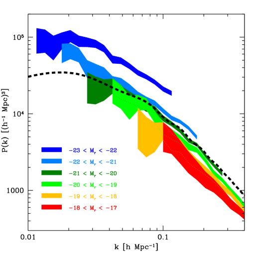
Figure 28.— The real-space power spectrum $P_{\rm gg}(k)$ is shown for galaxies in six bins of absolute magnitude $M_{{{}^{0.1}\!{r}}}$ detailed in Table 1, with the shading indicating $1-\sigma$ uncertainty. All power spectra have roughly the same shape, increasing in amplitude as the galaxies become more luminous. The dashed curve is the best fit linear $\Lambda$CDM model (see text) normalized to $\sigma_{8}=1$.

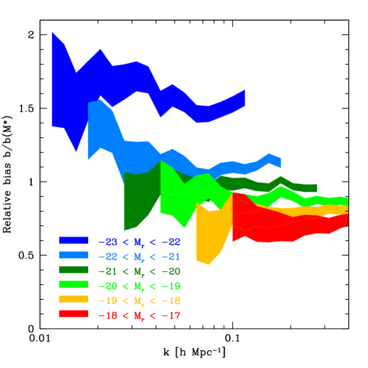
Figure 29.— The bias relative to the linear $\Lambda$CDM model of the previous figure is shown for galaxies in six bins of absolute magnitude $M_{{{}^{0.1}\!{r}}}$. All six curves are consistent with being scale-independent, the bias merely increasing in amplitude as the galaxies become more luminous.

5.1. Measurement of the luminosity-dependence of bias

To quantify the luminosity-dependence of bias for the SDSS galaxies, we repeat our entire analysis for each of the volume-limited samples L2-L7 specified in Table 1 and plotted in Section 2 (samples L1 and L8 contain too few galaxies to be useful). The resulting power spectra are shown in Figure 28. To avoid excessive clutter in this figure, we plot the minimum variance power spectrum estimate described in Appendix B.3.1. To indicate that the measurement errors are correlated between $k$-bins, we show the measurements as a shaded band rather than as separate points, with the vertical thickness of the band corresponding to the $1\sigma$ uncertainty. (The bias fitting below uses the full covariance matrix and is of course independent of what plotting convention is used, as is $\chi^{2}$ computed with equation (B15).)

Figure 28 shows that all power spectra have roughly the same shape, increasing in amplitude as the galaxies become more luminous. This is seen more clearly in Figure 29, where we have divided them all by the linear power spectrum of the simple $\Lambda$CDM reference model described below.

To quantify this similarity of shapes, we fit each of the measured power spectra to the reference $\Lambda$CDM curve with the amplitude freely adjustable. All six cases produce acceptable fits with reduced $\chi^{2}$ of order unity, and the corresponding best-fit normalizations are shown in Figure 30.

We want our reference model to provide an accurate empirical characterization of the SDSS data with as few parameters as possible. We choose it to be a flat scale-invariant $\Lambda$CDM model with the baryon density $h^{2}\Omega_{b}=0.024$ preferred by WMAP (Bennett et al. 2003) and the Hubble parameter $h=0.72$ preferred by the HST key project leaving $\Omega_{m}$ as the only free parameter determining its shape. We determine $\Omega_{m}$ by the following iterative procedure:

1. Given an $\Omega_{m}$-value, we compute the reference model $P(k)$ normalized to $\sigma_{8}=1$.

2. Given the reference model, we fit for the six bias factors plotted in Figure 30.

3. We fit these bias factors to a smooth curve $b(M)/b_{*}=A+B(L/L*)+C(M-M_{*})$ shown in Figure 30 given by the three parameters $(A,B,C)$.

4. We compute the correction $b_{\rm eff}(k)$ for scale-dependent bias shown in Figure 22 (top) as described below.

5. We compute the value of $\Omega_{m}$ that best fits the bias-corrected measurements in Figure 22 (bottom).

This procedure converges to within floating-point numerical precision in merely a few iterations for starting values anywhere in the range $0.1<\Omega_{m}<1.0$, yielding $\Omega_{m}=0.300$ and $(A,B,C)=(0.895,0.150,-0.040)$. The basic reason for this robustness is that changing the shape of the fiducial model changes $b_{\rm eff}(k)^{2}$ by a much smaller amount, because of the smearing by the integrals below.

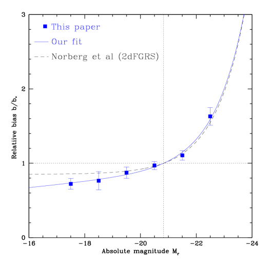
Figure 30.— The squares show the measured bias of our SDSS galaxies as a function of magnitude relative to $b_{*}$, the bias at $M*=-20.83$ (vertical dotted line). The solid curve shows the fit to our measurements described in the text, $b(M)/b_{*}=0.895+0.150L/L_{*}-0.040(M-M_{*})$, and the dashed curve shows the corresponding fit of Norberg et al. based on 2dFGRS data, $b(M)/b_{*}=0.85+0.15L/L*$.

5.2. Correcting for the luminosity-dependence of bias

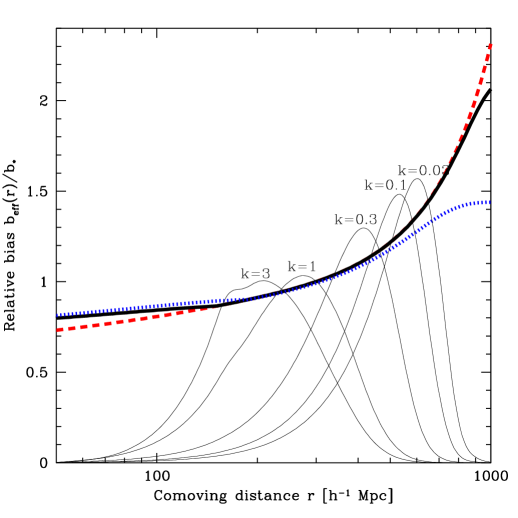
Figure 31.— The effective bias (equation 29; heavy curves) is seen to increase with distance, reflecting the fact that more distant galaxies are on average more luminous. The curves become shallower as the range of absolute magnitudes in the sample is cut, going from safe0 (dashed; no cuts) to safe13 (solid; $-23<M_{{{}^{0.1}\!{r}}}<-18.5$) to safe22 (dotted; $-22<M_{{{}^{0.1}\!{r}}}<-18$). Our volume-limited samples simply have $b_{\rm eff}(r)$ constant. The five thin curves show the relative weights given to different distances when measuring $P(k)$ for $k=0.03$, $0.1$, $0.3$, $1$ and $3h/{\rm Mpc}$ using the safe13 radial selection function.

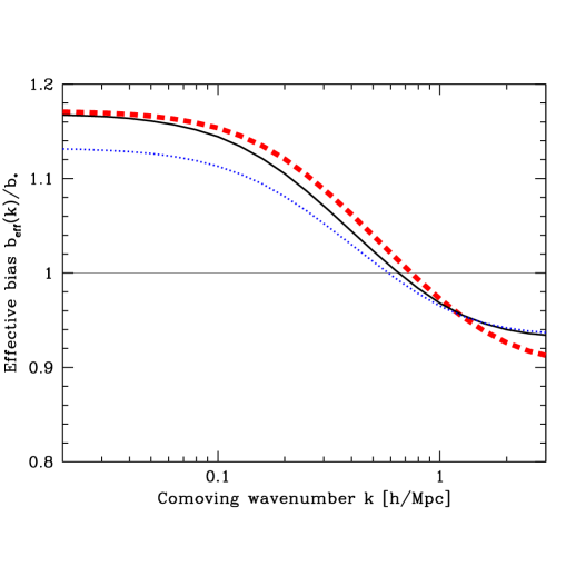
Figure 32.— The effective bias in the power spectrum measurement, equation (37), is seen to decrease with wavenumber $k$, reflecting the fact that low-$k$ measurements are dominated by more distant and luminous galaxies. The curves become shallower as the range of absolute magnitudes in the sample is cut, going from safe0 (thick dashed; no cuts) to safe13 (solid; $-23<M_{{{}^{0.1}\!{r}}}<-18.5$) to safe22 (dotted; $-22<M_{{{}^{0.1}\!{r}}}<-18$).

Above we quantified the well-known fact that the density field $\delta_{M}({\bf r})$ of galaxies of absolute magnitude $M$ is more strongly clustered for larger luminosity (smaller absolute magnitude $M$). Let us consider the simple bias model

$$\delta_{M}({\bf r})=b(M)\delta({\bf r}),$$ (26)

where $\delta({\bf r})$ is the field of matter fluctuations and $b(M)$ is the luminosity-dependent bias factor proportional to what is plotted in Figure 30. Since our observed galaxy sample mixes galaxies of various absolute magnitudes with some probability distribution $f_{M}(M;r)$, our observed density field can be written

$$\delta_{\rm obs}({\bf r})=\int f_{M}(M;r)\delta_{M}({\bf r})dM.$$ (27)

This probability distribution $f_{M}(M;r)$ is simply proportional to the galaxy luminosity function $\Phi(M)$ over the absolute magnitude range ${M_{\rm bri}}(r)<M<{M_{\rm dim}}(r)$ where the galaxy is observable at comoving distance $r$, zero otherwise, and normalized to integrate to unity. ${M_{\rm bri}}(r)$ and ${M_{\rm dim}}(r)$ are given by equation (A7) on inserting the appropriate absolute magnitude cuts from Table 1 (for instance, the sample safe13 has ${M_{\rm min}}=-23$, ${M_{\rm max}}=-18.5$). Substituting equation (26) into equation (27), we obtain

$$\delta_{\rm obs}({\bf r})=b_{\rm eff}(r)\delta({\bf r}),$$ (28)

where

$$b_{\rm eff}(r) = \int f_{M}(M;r)b(M)dM$$ (29)

$$= {\int_{{M_{\rm dim}}(r)}^{{M_{\rm bri}}(r)}\Phi(M)b(M)dM\over\int_{{M_{\rm dim}}(r)}^{{M_{\rm bri}}(r)}\Phi(M)dM}.$$

We evaluate this expression using the SDSS luminosity function measured in Blanton et al. (2002). The results are plotted in Figure 31, and the effective bias is seen to increase with distance as expected. We see that the curve $b_{\rm eff}(r)$ become shallower as the range of absolute magnitudes in the sample is cut, so the samples safe0, safe13 and safe22 are progressively less affected. Our volume-limited samples by construction simply have $b_{\rm eff}(r)={\rm constant}$.

Bias is expected to depend not only on luminosity but also on time (Fry 1996; Tegmark & Peebles 1998; Giavalisco et al. 1998; Cen & Ostriker 2000; Blanton et al. 2000). In addition, the intrinsic matter clustering should increase over time. Since the net result of these two counteracting effects is likely to be smaller than the luminosity effect at the low redshifts ($z\mathrel{\hbox to0.0pt{\lower 3.0pt\hbox{$\mathchar 536\relax$}\hss}\raise 2.0pt\hbox{$\mathchar 316\relax$}}0.2$) that we are considering, this is difficult to measure separately. The same applies to the small effect from the time-dependence of the redshift-space distortion parameter $\beta$ caused by the time-dependence of $\Omega_{m}$ and $\Omega_{\Lambda}$. Indeed, since typical luminosity grows monotonically with distance, the distance-dependent bias $b_{\rm eff}(r)$ plotted in Figure 31 should be expected to approximately include the combination of all four effects, so that our analysis will to first order be corrected for all of them.

Let us now estimate how $b_{\rm eff}(r)$ translates into $k$-dependent bias in our measured power spectrum. We do this in the FKP approximation (Feldman, Kaiser & Peacock 1994). Here the density field $\delta_{\rm obs}(r)$ is multiplied by a weight function

$$\phi(r)\propto{{\bar{n}}(r)P(k)\over 1+{\bar{n}}(r)P(k)}$$ (30)

and then Fourier transformed, giving

$$\int\phi(r)\delta_{\rm obs}({\bf r})e^{-i{\bf k}\cdot{\bf r}}d^{3}r=\int\phi(r)b_{\rm eff}(r)\delta({\bf r})e^{-i{\bf k}\cdot{\bf r}}d^{3}r$$ (31)

because of equation (28), so we see that we are simply measuring the power spectrum using a modified effective weight function, replacing $\phi$ by $\phi b_{\rm eff}$. It is well-known (see Tegmark et al. 1998 for a review conforming to the present notation) that the FKP estimate ${\tilde{P}}({\bf k})$ of the three-dimensional power spectrum $P({\bf k})$ satisfies

$$\langle{\tilde{P}}({\bf k})\rangle=(W\star P)({\bf k}),$$ (32)

i.e., that it probes the true power spectrum convolved with a window function $W({\bf k})$. This window function is the square modulus of the Fourier transform of the weight function, so it is given by

$$W_{0}({\bf k})\equiv|\widehat{\phi}({\bf k})|^{2},\quad W_{1}({\bf k})\equiv|\widehat{\phi b_{\rm eff}}({\bf k})|^{2},$$ (33)

where $W_{0}$ applies if we ignore bias and $W_{1}$ applies if we take bias into account. According to equation (32), galaxy bias therefore increases the measured power by a factor

$$b_{\rm eff}(k)^{2}={(W_{1}\star P)({\bf k})\over(W_{0}\star P)({\bf k})}={\int W_{1}({\bf k}^{\prime})P({\bf k}-{\bf k}^{\prime})d^{3}k^{\prime}\over\int W_{0}({\bf k}^{\prime})P({\bf k}-{\bf k}^{\prime})d^{3}k^{\prime}}.$$ (34)

The window function is normally narrower than the scale on which the power spectrum varies appreciably, so we can make the approximation of taking it out of the convolution integral, obtaining simply

$$b_{\rm eff}(k)^{2}={\int W_{1}({\bf k}^{\prime})d^{3}k^{\prime}\over\int W_{0}({\bf k}^{\prime})d^{3}k^{\prime}}={\int\phi(r)^{2}b_{\rm eff}(r)^{2}d^{3}r\over\int\phi(r)^{2}d^{3}r},$$ (35)

where we used Parseval’s theorem

$$\int|\widehat{\phi}({\bf k})|^{2}d^{3}k=(2\pi)^{3}\int|\phi(r)|^{2}d^{3}r$$ (36)

in the last step. In summary, substituting equation (30), we have shown that the effective bias as a function of wavenumber is

$$b_{\rm eff}(k)\approx\left[{\int\left({{\bar{n}}(r)P(k)\over 1+{\bar{n}}(r)P(k)}\right)^{2}b_{\rm eff}(r)^{2}r^{3}d\ln r\over\int\left({{\bar{n}}(r)P(k)\over 1+{\bar{n}}(r)P(k)}\right)^{2}r^{3}d\ln r}\right]^{1/2}.$$ (37)

The resulting curves $b_{\rm eff}(k)$ are plotted in Figure 32. As expected, the effective bias is seen to decrease with wavenumber $k$, reflecting the fact that low-$k$ measurements are dominated by more distant and luminous galaxies. Just as in the previous figure, the curves become shallower going from safe0 to safe13 to safe22, as the range of absolute magnitudes shrinks.

Note that if one treats $P(k)$ as a constant in equation (37), then $b_{\rm eff}(k)$ becomes a constant independent of $k$. Of the magnitude-limited galaxy survey analyses of the last decade, essentially the only one using such a constant weighting was the 2dFGRS analysis by Percival et al. (2001). Thus one can minimize the luminosity bias at the expense of increased statistical errors due to suboptimal galaxy weighting (as shown by Feldman, Kaiser & Peacock 1994, such uniform weighting is desirable only for volume-limited surveys where the galaxy number density is constant). In this paper we have instead used minimum-variance methods to measure the luminosity bias and power spectrum jointly. For a detailed discussion of these issues which appeared after the original version of this paper was submitted, see Percival et al. (2003).

The bottom line of this section is that although luminosity-dependent bias has only a small tilting effect on our measured SDSS power spectrum, we can and should correct for it when doing precision cosmology, by simply dividing the measured power spectrum by the square of the curve in the top panel of Figure 22. This correction curve has a slope around $-10\%$ per decade at $k\sim 0.2h/$Mpc. This means that fitting for cosmological parameters ignoring this effect would give noticeably biased results. For instance, assuming a power law primordial power spectrum of the form $k^{n_{s}}$, this would correspond to shifting the best fit spectral index ${n_{s}}$ by an amount $\Delta{n_{s}}\approx-(2/\ln 10)\times 10\%\approx-0.1$, and a more careful analysis in Section 7.3 shows the net effect to be $-0.06$. To place this in context, the popular stochastic eternal inflation model (Linde 1994) predicts ${n_{s}}\approx 0.96$, i.e., a substantially smaller departure from the ${n_{s}}=1$ scale-invariant case.

6. Tests for systematic errors in the data

The Monte Carlo experiments described in Section 4 provided an end-to-end validation of our method and our software. In this section, we turn to potential systematic errors in the SDSS data themselves. Examples of such effects include radial modulations (due to mis-estimates of evolution or $K$-corrections) and angular modulations (due to effects such as uncorrected dust extinction, variable observing conditions, photometric calibration errors and fiber collisions) of the density field.

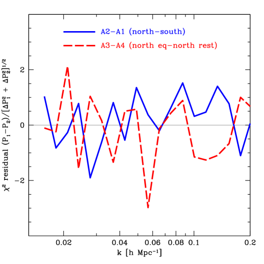
Figure 33.— Comparison of power in different parts of the sky defined by the angular subsamples A1-A4 in Table 1. Each curve shows the difference of two power spectra divided by the error bar on this quantity, so $\chi^{2}$ is simply the sum of the square of what is plotted. $\chi^{2}$ per degree of freedom is 0.86 for A2-A1 (north versus south) and 1.39 for A3-A4 (the two separate northern regions).

6.1. Analysis of subsets of galaxies

Since such effects would be expected to vary across the sky (depending on, say, reddening, seasonally variable baseline offsets or observing conditions such as seeing and sky brightness), we repeat our entire analysis for four different angular subsets of the sky (subsamples A1-A4 from Table 1) in search of inconsistencies. We subtract the power spectrum measured south of the Galactic plane (A1) from the power spectrum measured north of the Galactic plane (A2) for $k<0.2h/$Mpc using the modeling method, and obtain a residual $\chi^{2}\approx 16$ for 19 degrees of freedom. A similar comparison of the two disjoint northern regions (A3 and A4) gives a residual $\chi^{2}\approx 26$, again for 19 degrees of freedom. Under the null hypothesis that a such a pair of curves are independent measurements of the same underlying power spectrum, the mean and standard deviation is $\langle\chi^{2}\rangle=19$ and $\Delta\chi^{2}=(2\times 19)^{1/2}\approx 6$, so these residuals are $-0.4$ and $+1.4$ standard deviations away from the expectation, respectively. In other words, there is no significant evidence for discrepancies between the power spectra measured in different parts of the sky.

The actual residuals are shown in Figure 33. Since our measurements in different $k$-bands are uncorrelated, $\chi^{2}$ is simply the sum of the square of what is plotted. The most notable discrepancy is at $k\sim 0.05h/$Mpc, where there is more power in A4 than in A3. This appears to be related to a striking wall-like structure that is seen in the northern galaxy distribution around $z\sim 0.08$ (see Figure 5). Although this “great blob” may be the largest coherent structure yet observed, a first crude estimate suggests that it is not inconsistent with Gaussian fluctuations: visual inspection of the 275 PThalos simulations reveals similar structures in more than $10\%$ of the cases.

A similar comparison of the power spectra in the radial subsamples R1-R3 is less useful, since this radial binning is largely degenerate with the luminosity binning (Section 5), so we test for radial systematics with mode subsets instead.

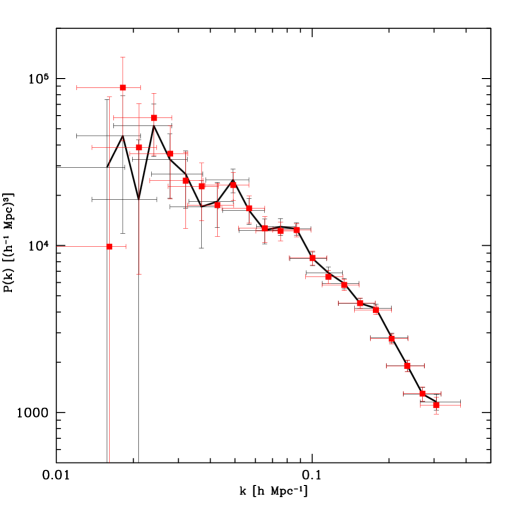
Figure 34.— Effect of removing special modes. Black curve with associated error bars shows our measured power spectrum $P_{\rm gg}(k)$ from the modeling method using all 4000 PKL modes. Red squares with error bars show the effect of removing the 234 special modes corresponding to purely angular and purely radial fluctuations as well as fluctuations associated with the motion of the Local Group relative to the CMB rest frame. Any systematic errors adding power to these special modes would cause the curve to lie systematically above the squares.

6.2. Analysis of subsets of modes

Because of their angular or radial nature, all potential systematic errors discussed above create excess power mainly in the radial and angular modes. To quantify any such excess, we therefore repeat our entire analysis with all 233 special modes (27 radial modes, 199 angular modes and 7 Local Group modes) deleted. The results of this test are shown in Figure 34 and are very encouraging; the differences are tiny. Any systematic errors adding power to these special modes would cause the squares to lie systematically above the crosses, yet the squares fall below the crosses for four out of the five leftmost bands, where such systematics would be most important. Thus there is no indication of excess radial or angular power in the data.

Figure 34 shows that removing the special modes results in a slight error bar increase on the largest scales and essentially no change on smaller scales. This can be readily understood geometrically. If we count the number of modes that probe mainly scales $k<k_{*}$, then the number of purely radial, purely angular and arbitrary modes will grow as $k_{*}$, $k_{*}^{2}$ and $k_{*}^{3}$, respectively. This means that “special” modes (radial and angular) will make up a larger fraction of the total pool on large scales (at small $k$), and that the purely radial ones will be outnumbered by the purely angular ones.

Our treatment of spectroscopic fiber collisions described in Appendix A is another source of potential angular/radial problems. By assigning both members of some close pairs (separated by less than $55^{\prime\prime}$, corresponding to $0.08h^{-1}$Mpc at the mean depth of the survey) at the same redshift, we overestimate the radial power on small scales. Zehavi et al. (2002) perform extensive tests of this effect and show that it is negligible on large scales considered in this paper. As a further cross-check, we repeat our entire calculation with all galaxies with such assigned redshifts removed. Since this second approach is guaranteed to underestimate the power, the two approaches will bracket the correct answer. As expected based on the Zehavi et al. (2002) analysis, we find no evidence that fiber collisions are boosting our measured power spectrum on the smallest scales we probe ($k\sim 0.3h/$Mpc).

7. Discussion and conclusions

7.1. Basic results

We have measured the shape of the real-space power spectrum $P(k)$ on large scales using the SDSS galaxy redshift catalog, paying particular attention to quantifying and correcting for the effects of survey geometry, redshift space distortions and luminosity-dependent bias. Our principal results are the estimates $P_{\rm gg}(k)$ of the real space galaxy power spectrum which are listed in Tables 2 and 3 for the disentanglement and modeling methods, respectively. As discussed in Section 4, the disentanglement method is more robust, but the modeling method (Figure 22) yields smaller statistical errors and appears in our tests to introduce little systematic error. Table 3 lists results both for FOG compression with $\delta_{c}=200$, which we consider the most reliable choice for estimating the true real space power spectrum, and for no FOG compression, which is the case easiest to model in detail. Our estimation procedure yields uncorrelated error bars, so the reported errors in these tables can be used as a diagonal covariance matrix when evaluating the likelihood for model fits. For such fits, it is crucial to use the exact window functions, which are available at
http://www.hep.upenn.edu/$\sim$max/sdss.html together with sample software for evaluating the SDSS likelihood function.

As noted in Section 4, uncertainties in the values of $\beta$ and $r$ leave a $4\%$ $1\sigma$ uncertainty in the overall normalization of $P_{\rm gg}(k)$ with the modeling method, in addition to the error bars on individual points. There is no corresponding normalization uncertainty for the disentanglement method. Our tabulated power measurements have all been corrected for the effect of luminosity-dependent bias as discussed in Section 5. The correction $b(k)$ used is given in Tables 2 and 3, and is normalized so that our quoted power measurements represent the power spectrum of galaxies with absolute r-band magnitude $M_{*}\approx-20.83$; the relative bias of galaxies as a function of luminosity can be found in Figure 30.

7.2. Using our results

There are several levels at which one might use our results, depending on how conservative one wishes to be and how much energy one has for theoretical modeling. The mock catalog tests in Section 4.2 (Figure 27 in particular) suggest that our method is quite successful at correcting for redshift space distortions to recover the real space galaxy power spectrum $P^{\rm true}_{\rm gg}(k)$. However, there are notable departures from perfect recovery at $k\mathrel{\hbox to0.0pt{\lower 3.0pt\hbox{$\mathchar 536\relax$}\hss}\raise 2.0pt\hbox{$\mathchar 318\relax$}}0.15h/$Mpc, and the tests are in any event carried out for a particular choice of cosmology and galaxy bias model. The simplest and least conservative way to use our results is to assume that we have indeed recovered $P^{\rm true}_{\rm gg}(k)$ and to further assume that on the scales of our measurement the galaxy power spectrum is a scale-independent multiple of the linear theory matter power spectrum, $P_{\rm gg}(k)=b_{*}^{2}P(k)$ where $b_{*}$ represents the large scale bias factor of $L_{*}$ galaxies. The agreement of the lines representing $P_{\rm gg}(k)$ and the linear $P(k)$ in Figure 27 suggests that this approach is probably safe for $k\mathrel{\hbox to0.0pt{\lower 3.0pt\hbox{$\mathchar 536\relax$}\hss}\raise 2.0pt\hbox{$\mathchar 316\relax$}}0.1h/{\rm Mpc}$, and that one can use the more precise modeling estimates of $P_{\rm gg}(k)$ (Table 3) without incurring a systematic error that is significant relative to the statistical errors of the current measurement. However, our tests are not exhaustive, and it is possible that the agreement of $P_{\rm gg}(k)$ and linear $P(k)$ shapes in Figure 27 arises in part from a cancellation of non-linear gravitational effects with errors in the redshift-space distortion correction. This cancellation, in turn, might not hold for other cosmological or galaxy bias models.

A second option is to assume that we have recovered $P^{\rm true}_{\rm gg}(k)$ but not assume that this has the same shape as the linear theory matter power spectrum. Here, for example, one could use N-body simulations or analytic approximations to compute the non-linear, real space power spectrum, incorporating galaxy bias based on semi-analytic galaxy formation calculations, hydrodynamic simulations, or a “halo occupation” model constrained by other measurements of galaxy clustering. Figure 27 again suggests that this approach can be used safely for $k\mathrel{\hbox to0.0pt{\lower 3.0pt\hbox{$\mathchar 536\relax$}\hss}\raise 2.0pt\hbox{$\mathchar 316\relax$}}0.1h/$Mpc (and perhaps a bit further) without systematic errors that exceed the statistical errors. One can also use the non-linear matter power spectrum and a constant $b$, but there is good reason to expect scale-dependent bias on scales where non-linearity is significant (Hamilton & Tegmark 2002). Finally, the most cumbersome but most reliable way to use our data is to follow the course suggested at the end of Section 4: create redshift-space realizations using non-linear simulations with galaxy bias, compute the monopole, quadrupole, and hexadecapole components of the redshift space power spectrum in the distant observer approximation, and use equation (17) to convert them to $P_{\rm gg}(k)$. These predictions should be compared directly to the disentanglement estimates of $P_{\rm gg}(k)$, since the redshift-space distortions have been incorporated into the model rather than removed from the data. However, by focusing on a quantity $P_{\rm gg}(k)$ that responds mainly to real space clustering (exactly so in the linear regime), such a comparison will be insensitive to moderate errors in the redshift-space distortions incorporated in the theoretical predictions. This last approach is still much simpler than creating artificial SDSS catalogs and reproducing our estimation method in its entirety, but it should be equally valid.

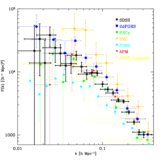
Figure 35.— Comparison with other galaxy power spectrum measurements. Numerous caveats must be borne in mind when interpreting this figure. Our SDSS power spectrum measurements are those from Figure 22, corrected for the red-tilting effect of luminosity dependent bias. The purely angular analyses of the APM survey (Efstathiou & Moody 2001) and the SDSS (the points are from Tegmark et al. 2002 for galaxies in the magnitude range $21<r^{*}<22$ — see also Dodelson et al. 2002) should also be free of this effect, but represent different mixtures of luminosities. The 2dFGRS points are from the analysis of HTX02, and like the PSCz points (HTP00) and the UZC points (THX02) have not been corrected for this effect, whereas the Percival et al. 2dFGRS analysis should be unafflicted by such red-tilting. The influential PD94 points (Table 1 from Peacock & Dodds 1994), summarizing the state-of-the-art a decade ago, are shown assuming IRAS bias of unity and the then fashionable density parameter $\Omega_{m}=1$.

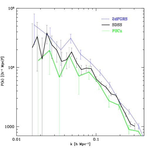
Figure 36.— Same as Figure 35, but restricted to a comparison of decorrelated power spectra, those for SDSS, 2dFGRS and PSCz. The similarity in the bumps and wiggles between the three power spectra is intriguing.

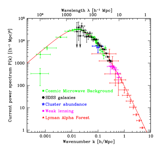
Figure 37.— Comparison of our results with other $P(k)$ constraints. The location of CMB, cluster, lensing and Ly$\alpha$ forest points in this plane depends on the cosmic matter budget (and, for the CMB, on the reionization optical depth $\tau$), so requiring consistency with SDSS constrains these cosmological parameters without assumptions about the primordial power spectrum. This figure is for the case of a “vanilla” flat scalar scale-invariant model with $\Omega_{m}=0.28$, $h=0.72$ and $\Omega_{b}/\Omega_{m}=0.16$, $\tau=0.17$ (Spergel et al. 2003; Verde et al. 2003, Tegmark et al. 2003b), assuming $b_{*}=0.92$ for the SDSS galaxies.

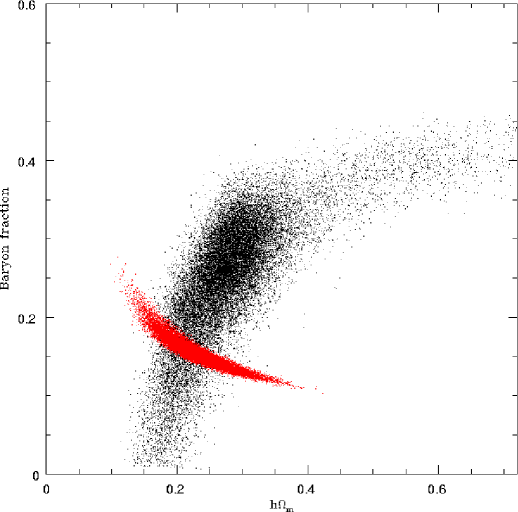
Figure 38.— Characterization of the SDSS power spectrum in terms on constraints on the “shape parameter” $h\Omega_{m}$ and the baryon fraction $f_{b}$. Black points show 100,000 Markov Chain steps for SDSS, red/grey points are for WMAP data.

7.3. Comparison to other results

Figure 35 compares our results from Table 3 (modeling approach) with other measurements from galaxy surveys, but must be interpreted with care. The UZC points may contain excess large-scale power due to selection function effects (Padmanabhan et al. 2000; THX02), and the angular SDSS points measured from the early data release sample are difficult to interpret because of their extremely broad window functions. Only the SDSS, APM and angular SDSS points can be interpreted as measuring the large-scale matter power spectrum with constant bias, since the others have not been corrected for the red-tilting effect of luminosity-dependent bias. The Percival et al. (2001) 2dFGRS analysis unfortunately cannot be directly plotted in the figure because of its complicated window functions.

Figure 36 is the same as Figure 35, but restricted to a comparison of decorrelated power spectra, those for SDSS, 2dFGRS and PSCz. Because the power spectra are decorrelated, it is fair to do “chi-by-eye” when examining this Figure. The similarity in the bumps and wiggles between the three power spectra is quite striking. Moreover, there is an interesting degree of similarity with the power spectrum of the Abell/ACO cluster catalog (not shown) reported by Miller & Batuski (2001). It is tempting to see hints of baryonic oscillations in these wiggles. Indeed Percival et al. (2001) in their analysis of the 2dFGRS, and Miller et al. (2001a,b; see also Miller et al. 2002) in their analysis of the Abell/ACO cluster (Miller & Batuski (2001), APM cluster (Tadros, Efstathiou & Dalton 1998), and PSCz surveys (HTP00), already concluded that their data mildly preferred model power spectra with baryonic oscillations over those without. However, the oscillations at large scales evident in Figure 36, notably the dip at $k\sim 0.035\,h{\rm Mpc}^{-1}$ and bump at $k\sim 0.05\,h{\rm Mpc}^{-1}$, are substantially larger than predicted by the standard $\Lambda$CDM concordance model illustrated in Figure 22; if confirmed, such a feature would challenge the $\Lambda$CDM concordance model with scale-invariant initial conditions. This preference for a large baryon fraction is also seen in Figure 38 (details below) which, however, shows that our SDSS data is nonetheless perfectly consistent with the concordance baryon fraction — about one sixth of the 100,000 points shown have a baryon fraction below the WMAP value of $17\%$.

Figure 38 also illustrates why galaxy clustering data is so complementary to CMB measurements. The 100,000 red/grey points are from a Monte Carlo Markov Chain analysis of the WMAP for simple flat scalar adiabatic models parametrized by the densities of dark energy, dark matter and baryronic matter, the spectral index and amplitude, and the reionization optical depth. As emphasized by Eisenstein et al. (1999) and Bridle et al. (2003), WMAP alone cannot determine $\Omega_{m}$ to better than a factor of two or so because of a strong degeneracy with other parameters. Fortunately, the WMAP degeneracy banana in Figure 38 is seen to be almost orthogonal to the SDSS degeneracy, which means that combining the two measurements dramatically tightens the constraints on all the parameters involved in the degeneracy — notably $\Omega_{m}$, $h$ and $\sigma_{8}$.

To place our SDSS results in a larger context, Figure 37 compares them with other measurements of the matter power spectrum $P(k)$. Here the CMB, galaxy cluster, lensing and Ly$\alpha$ forest results have been mapped into $k$-space using the method of Tegmark & Zaldarriaga (2002), assuming the WMAP model given in the caption, and we have assumed an SDSS bias $b_{*}=1$. The CMB data combines the Boomerang, MAXIMA, DASI, CBI, VSA, ACBAR and WMAP data as in Wang et al. (2002) with the WMAP measurements (Hinshaw et al. 2003). The cluster point reflects the spread in the recent literature rather than any one quoted measurement. The lensing data are from Hoekstra et al. (2002). The Ly$\alpha$ forest points are from the Gnedin & Hamilton (2002) reanalysis of the Croft et al. (1999) data.

We leave detailed investigation of the implications of our measurement to other papers (by ourselves in Paper II and, we hope, by others), since the primary goal of this paper is the measurement itself. As a characterization of our data, we will briefly indulge in the simplest of the interpretive approaches described in Section 7.2. For this purpose, we fit our 22 $P_{\rm gg}(k)$-measurements derived from the modeling method with $\delta_{c}=200$ using the linear CDM power spectrum of Eisenstein & Hu (1999), fixing the baryon fraction $\Omega_{b}/\Omega_{m}=0.17$ and the Hubble parameter $h=0.72$ as per the best fits from WMAP (Bennett et al. 2003; Spergel et al. 2003; Verde et al. 2003) and no massive neutrino contribution. If we further fix the inflationary spectral index to ${n_{s}}=1$, then the shape of $P(k)$ is determined by the combination $h\Omega_{m}$, and we find $h\Omega_{m}=0.201\pm 0.017$ at $1\sigma$, i.e., $\Omega_{m}=0.300\pm 0.018$.

As discussed above, our modeling of nonlinear redshift space distortions is only accurate on large scales, so we recommend not using the measurements with $k>0.2h/{\rm Mpc}$ for cosmological analysis. In this spirit, we fit the 19 $P_{\rm gg}(k)$-measurements for $k<0.2h/{\rm Mpc}$ to the two-parameter model defined by the Smith et al. (2003) nonlinear power spectrum approximation using the Eisenstein & Hu (1999) fit as above for the linear transfer function, fixing the bias $b_{*}=1$. This gives the shape parameter $h\Omega_{m}=0.213\pm 0.0233$ at $1\sigma$, i.e., $\Omega_{m}=0.295\pm 0.0323$. This fit has $\chi^{2}=15.6$ for $19-2=17$ effective degrees of freedom, so this two-parameter model fit can be regarded as an adequate representation of our results in compact summary form. (Using a linear power spectrum model would increase this $\Omega_{m}$-value by $0.043$.) Figure 38, which was commented on above, shows the result of repeating this same fit after adding the baryon fraction as a third free paramenter. Fixing the best-fit shape $h\Omega_{m}=0.213$, the power spectrum amplitude corresponds to $\sigma_{8}=0.89\pm 0.02$ for $L^{*}$ galaxies after marginalizing over the redshift-space distortion parameters $\beta$ and $r$. Note that this normalization is at the effective redshift of the survey, not for $z=0$ galaxies.

If we fix $\Omega_{m}$ at the best-fit value $0.291$ and treat the spectral index as the free shape parameter, then we find ${n_{s}}=0.995\pm 0.049$. Without our correction for luminosity-dependent bias, the corresponding numbers are ${n_{s}}=0.933\pm 0.046$, so the statistical errors are now small enough for effects such as this to be important. Similarly, Table 7 of Paper II shows that ignoring this correction reduces the measured value of $\Omega_{m}$ by $0.035$.

Paper II presents a thorough analysis of the cosmological constraints from our $P(k)$-measurement, finding them in good agreement with a “vanilla” flat adiabatic $\Lambda$CDM model with neglibible tilt, running tilt, tensor modes or massive neutrinos. Our $P(k)$ measurement provides a powerful confirmation of the results reported by the WMAP team, and more than halves the WMAP-only error bars on some parameters, e.g., the matter density $\Omega_{m}$ and the Hubble parameter $h$. Paper II finds $\Omega_{m}=0.30\pm 0.04$ from WMAP+SDSS when marginalizing over the other “vanilla” parameters. This is about $1\sigma$ higher that when using the 2dFGRS survey (which gave a slightly redder $P(k)$ slope than we found) — just the sort of statistical difference one would expect from two completely independent samples.

7.4. Outlook

Let us conclude by looking ahead. Galaxy surveys have the potential to greatly improve the cosmological constraints from the cosmic microwave background by breaking degeneracies and providing cross-checks, so detailed joint analysis of our measurements with WMAP and other data sets will be worthwhile. In particular, detecting the effect of baryons on $P(k)$ (Tegmark 1997a; Goldberg & Strauss 1998) can provide powerful constraints on the Hubble parameter (Eisenstein et al. 1998) and accurate determination of the shape of $P(k)$ can place strong constraints on neutrino masses (Hu et al. 1998; Spergel et al. 2003; Hannestad 2003) and help pin down the primordial power spectrum. Deeper surveys can also provide interesting constraints on the evolution of clustering and dark energy, and the SDSS luminous red galaxy (LRG) sample and photometric redshift catalog will complement specialized deep redshift surveys such as DEEP (Davis et al. 2001) and VIRMOS (Le Fèvre et al. 2001) in this regard.

Prospects are also good for reducing systematic uncertainties involving both bias and redshift distortions. A key virtue of having very large galaxy samples is it permits accurate measurements for large numbers of subsamples. For instance, repeating our analysis for subsamples based on galaxy color or spectral type will provide a powerful test of how scale-independent the bias is on large scales. Moreover, empirical constraints from SDSS on redshift-space distortions should improve substantially. These constraints are currently rather weak because the survey geometry consists largely of thin wedges; we have therefore focused simply on modeling distortions well enough to remove their impact on the real space $P(k)$ estimate. As the survey area fills in and becomes more contiguous, we expect to obtain interesting constraints on redshift distortions that can be used to test and refine theoretical and numerical models.

In addition to more careful modeling and combining with other observational constraints, we anticipate several complementary results from the SDSS in the near future, such as cosmological constraints directly from KL-modes (Pope et al. 2003), real space clustering on small scales from the projected correlation function $w(r_{p})$ (Zehavi et al. 2003b), power spectrum measurements on large scales using the luminous red galaxy sample and angular clustering measurements using photometric redshifts (Budavari et al. 2003). This should help break degeneracies and provide cross-checks to test rather than assume the physics underlying the cosmological model, thereby strengthening the weakest link in post-WMAP cosmology.

We wish to thank Adrian Jenkins and Carlton Baugh for providing Hubble Volume simulation results and Scott Dodelson for useful suggestions. MT thanks Angelica de Oliveira-Costa for helpful comments and infinite patience.

Funding for the creation and distribution of the SDSS Archive has been provided by the Alfred P. Sloan Foundation, the Participating Institutions, the National Aeronautics and Space Administration, the National Science Foundation, the U.S. Department of Energy, the Japanese Monbukagakusho, and the Max Planck Society. The SDSS Web site is http://www.sdss.org/.

The SDSS is managed by the Astrophysical Research Consortium (ARC) for the Participating Institutions. The Participating Institutions are The University of Chicago, Fermilab, the Institute for Advanced Study, the Japan Participation Group, The Johns Hopkins University, Los Alamos National Laboratory, the Max-Planck-Institute for Astronomy (MPIA), the Max-Planck-Institute for Astrophysics (MPA), New Mexico State University, University of Pittsburgh, Princeton University, the United States Naval Observatory, and the University of Washington.

MT was supported by NSF grants AST-0071213 & AST-0134999, NASA grants NAG5-9194 & NAG5-11099 and fellowships from the David and Lucile Packard Foundation and the Cottrell Foundation. MAS acknowledges support from NSF grant AST-007109, and AJSH from NSF grant AST-0205981 and NASA grant NAG5-10763. Our PThalos mock catalogs were created on the NYU Beowulf cluster supported by NSF grants PHY-0116590 and PHY-0101738, and NASA grant NAG5-12100.

A. Data and data modeling

In this Appendix, we provide a detailed description of how our basic galaxy sample was processed, modeled and split into the subsamples used in our power spectrum analysis.

A.1. The SDSS Galaxy Catalog

The SDSS (York et al. 2000) is producing imaging and spectroscopic surveys over about a quarter of the Celestial Sphere. A dedicated 2.5m telescope at Apache Point Observatory, Sunspot, New Mexico, images the sky in five bands between 3,000AA and 10,000AA ($u$, $g$, $r$, $i$, $z$; Fukugita et al. 1996) using a drift-scanning, mosaic CCD camera (Gunn et al. 1998), detecting objects to a flux limit of $r\sim 22.5$. The photometric quality of the observations are tracked using an automatic photometricity monitor (Hogg et al. 2001). One of the goals is to spectroscopically observe 900,000 galaxies, (down to $r_{\mathrm{lim}}\approx 17.77$; Strauss et al. 2002), 100,000 Luminous Red Galaxies (LRGs; Eisenstein et al. 2001), and 100,000 QSOs (Richards et al. 2002). This spectroscopic follow-up uses two digital spectrographs (Uomoto et al. 2003) on the same telescope as the imaging camera. Other aspects of the survey are described in the Early Data Release (EDR) paper (Stoughton et al. 2002).

The SDSS images are reduced and catalogs are produced by the SDSS pipeline photo (Lupton et al. 2001), which detects and measures objects, the sky background, and the seeing conditions. As described in Smith et al. (2002), magnitudes are calibrated to a standard star network approximately in the $AB$ system. The astrometric calibration is also performed by an automatic pipeline which obtains absolute positions to better than 0.1 arcsec rms per coordinate (Pier et al. 2003).

Object fluxes are determined in several different ways by photo, as described in Stoughton et al. (2002). The primary measure of flux used for galaxies is the SDSS Petrosian magnitude, a modified version of the quantity proposed by Petrosian (1976). In the absence of seeing, Petrosian magnitudes measure a constant fraction of a galaxy’s light regardless of distance (or size). They are described in greater detail by Blanton et al. (2001) and Strauss et al. (2002). Another important measure of flux for galaxies is the SDSS model magnitude, which is an estimate of the magnitude using the better of a de Vaucouleurs and an exponential fit to the image. Finally, the SDSS also measures the flux in each object using the local PSF as a template, which is the highest signal-to-noise ratio measurement of flux for point sources.

Main sample target selection (Strauss et al. 2002) involves star/galaxy separation, application of the flux limit, application of the surface brightness limit and application of the fiber magnitude limit. Expressed quantitatively, the first three of these criteria are

$$r_{\mathrm{PSF}}-r_{\mathrm{model}} > s_{\mathrm{limit}}$$ (A1)

$$r_{\mathrm{petro}} < r_{\mathrm{limit}},\mathrm{~{}and}$$ (A2)

$$\mu_{50} < \mu_{50,\mathrm{limit}}.$$ (A3)

where $r_{\mathrm{petro}}$ is the dereddened Petrosian magnitude in the $r$ band (using the dust maps of Schlegel, Finkbeiner & Davis 1998), $r_{\mathrm{model}}$ is the model magnitude, $r_{\mathrm{PSF}}$ is the PSF magnitude, and $\mu_{50}$ is the Petrosian half-light surface brightness of the object in the $r$-band. In practice, the values of the target selection parameters vary across the survey in a well-understood way, but for the bulk of the area, they are $s_{\mathrm{limit}}=0.3$, $r_{\mathrm{limit}}=17.77$, and $\mu_{50,\mathrm{limit}}=24.5$. We note here that objects near the spectroscopic flux limit are nearly five magnitudes brighter than the photometric limit; that is, the fluxes are measured at a signal-to-noise ratio of a few hundred.

Fibers are assigned to a set of circular tiles with a field of view $1.49^{\circ}$ in radius by an automatic tiling pipeline (Blanton et al. 2003). The targets are observed using a 640 fiber spectrograph on the same telescope as the imaging camera. We extract one-dimensional spectra from the two-dimensional spectrograms using a pipeline (idlspec2d) created specifically for the SDSS instrumentation (Schlegel et al. 2003); a further pipeline (specBS v4_9) fits for the redshift of each spectrum. The official SDSS redshifts are obtained from a different pipeline (Frieman et al. 2003). The two independent versions provide a consistency check on the redshift determination. They are consistent (for galaxies) at over the 99% level.

Fibers on a single plate cannot be placed more closely than $55^{\prime\prime}$. Thus, redshifts for both members of a close galaxy pair can only be obtained in regions where tiles overlap. If we did not take fiber collisions into account at all, we would systematically underestimate correlations on all scales. We correct this bias by assigning each galaxy pair member whose redshift was not obtained because of a fiber collision the same redshift as the pair member whose redshift was measured.Thus, for 192,642 of the galaxies in the full sample, a spectroscopic redshift is available, but for 12,801 ($\sim 6\%$) we must assign redshifts according to this prescription. Using the overlaps of multiple tiles, where many of these pairs can be recovered, Zehavi et al. (2002) have shown that this procedure works well on large scales, and we confirm this conclusion with additional tests in Section 6.

As of July 2002, the SDSS had imaged and targeted 2,873 deg² of sky and taken 431,291 successful spectra (including 323,126 spectra of galaxies) over $2{,}499$ deg² of that area. We created a well-defined sample for calculating large-scale structure and galaxy property statistics from these data, known as Large-Scale Structure sample11. sample11 consists of all of the photometry for all of the targets over that area (as extracted from the internal SDSS operational database), all of the spectroscopic results (as output from idlspec2d), and a description of the angular window function of the survey and the flux and surface brightness limits used for galaxies in each area of the sky (discussed more fully below). For most of the area, we used the same version of the analysis software that was used to create the target list. However, for the area covered by the Early Data Release (EDR; Stoughton et al. 2002) we used the version of the analysis software used for that data release, since it was substantially better than the early versions of the software used to target that area. For photo, the most important piece of analysis software run on the data, the versions used for the photometry range from v5_0 to v5_2. The region covered by this sample is similar to, but somewhat greater than, the region which will be released in the SDSS Data Release 1 (DR1), (which will use a newer version of the software which among other things improves the handling of large galaxies). For all of the subsamples of sample11 defined here, we define a bright limit of $r=14.5$ (using Petrosian, dereddened magnitudes) to exclude the spectroscopic bright limits imposed in galaxy target selection as well as the possibility of poor deblending of bright objects by photo (a problem for v5_2 and previous, though less so for v5_3).

We measure galaxy magnitudes through a set of bandpasses that are constant in the observer frame. These observer frame magnitudes correspond to different rest-frame magnitudes depending on the galaxy redshift. In order to compare galaxies observed at different redshifts, we convert all the magnitudes to a single fixed set of bandpasses using the method of Blanton et al. (2002b) (kcorrect v1_11). These routines fit a linear combination of four spectral templates to each set of five magnitudes. The coefficient $a_{0}$ of the first template is an estimate of the flux in the rest-frame optical range ($3500{\rm AA}<\lambda<7500{\rm AA}$), the fractional contribution of the other coefficients $a_{1}/a_{0}$, $a_{2}/a_{0}$, and $a_{3}/a_{0}$ characterize the spectral energy distribution of the galaxy. The most significant variation is along $a_{3}/a_{0}$. Taking the sum of the templates and projecting it onto filter responses, we can calculate the $K$-corrections from the observed bandpass to any rest-frame bandpass. In practice, for the rare galaxies in our sample around redshift $z\sim 0.3$ this procedure is unstable. Thus, for this sample we fix the coefficients for all galaxies at redshifts $z>0.28$ to the average value for galaxies between redshifts $0.26<z<0.28$, corresponding to the typical red luminous galaxy SED. The median redshift of the sample is 0.1, so in this paper, we quote absolute magnitude restframe bandpasses shifted blueward from the observatory frame bandpasses by a factor 1.1 and denoted ${{}^{0.1}\!{r}}$ in $r$-band. This procedure minimizes the uncertainties in the $K$-corrections, since galaxies near the median redshift independent of their spectral energy distribution. For a galaxy exactly at $z=0.1$, the $K$-corrections are trivial.

In the remainder of this section, we model the three-dimensional selection function ${\bar{n}}({\bf r})$, which gives the expected number density of galaxies in the absence of clustering as a function of three-dimensional position. For a uniform magnitude limit, our selection function is separable into the product of an angular part and a radial part:

$${\bar{n}}({\bf r})={\bar{n}}(\widehat{\bf r}){\bar{n}}(r),$$ (A4)

where ${\bf r}\equiv r\widehat{\bf r}$ and $\widehat{\bf r}$ is a unit vector. The angular part ${\bar{n}}(\widehat{\bf r})$ may take any value between 0 and 1, and gives the completeness as a function of position, i.e., the fraction of all survey-selected galaxies for which survey quality redshifts are actually obtained, while ${\bar{n}}(r)$ gives the radial selection function. As described in Section 6, this separability allows powerful tests for possible systematic effects arising from extinction or calibration problems, which would cause a purely angular modulation of density fluctuations, or from a mis-estimate of the radial selection function, which would cause a purely radial modulation of the density. The SDSS spectroscopic completeness is so good that we find no evidence for weather-related effects breaking the separability as in the 2dFGRS (Colless et al. 2001), and therefore do not need to perform corrections for this effect as in THX02. We will now describe our modeling of the two factors ${\bar{n}}(\widehat{\bf r})$ and ${\bar{n}}(r)$ in turn.

A.2. The angular selection function

A.2.1 Specification

The geometry of the survey is somewhat complex due to the fact that the imaging and spectroscopy programs are carried out concurrently. To supply targets for the spectroscopic program, periodically a “target chunk” of imaging data is processed, calibrated, and has targets selected. These target chunks never overlap, so that once a set of targets is defined in a particular region of sky, it never changes in that region. Thus, the task of determining the selection limits used in any region reduces to tracking how the target chunks cover the sky. This list of target chunks, their boundaries, and their selection criteria is an important product of sample11.

To drill spectroscopic plates which have fibers on these targets, we define “tiling chunks” which in principle can overlap more than one target chunk. The tiling algorithm (Blanton et al. 2003) is then run in order to position tiles and assign fibers to them, after which plates are designed (that is, any available fibers are assigned to various classes of auxiliary targets as well as to sky and calibration stars) and then drilled. In general, these tiling chunks will overlap because we want the chance to assign fibers to targets which may have been in adjacent, earlier tiling chunks but were not assigned a fiber. For a target to be covered by a particular tile, it must be in the same tiling chunk as that tile and be within the area of the tile itself (because the edges of tiles can extend beyond the tiling chunk boundaries, a particular region of sky can be within the area of a tile but not “covered” by it as defined here). We then divide the survey into a number of “sectors”, regions which are covered by a unique set of tiles and tiling chunks (following the nomenclature of the 2dFGRS, Percival et al. 2001, the “sectors” are the same as the “overlap regions” defined in Blanton et al. 2001a). For instance, two tiles overlapping each other but no other tiles give rise to three sectors: the area covered only by the first tile, the area covered only by the second tile, and the area covered by both.

For sample11  the sky area is covered by 669 circular tiles of diameter $2.98^{\circ}$ and is split into 2489 disjoint sectors. This decomposition is convenient since each sector has a unique sampling rate. The sampling rate of a sector is defined as the number of redshifts of galaxy targets obtained in the sector (including the galaxies assigned the redshift of a neighbor because of a fiber collision) divided by the number of galaxy targets in the sector. The sampling rate so calculated is about 95% on average across the survey area; about 95% of the survey area has completeness greater than 90%. This is illustrated in Figure 1.

Two additional sets of geometric entities affect the angular selection function ${\bar{n}}(\widehat{\bf r})$: it vanishes inside each of 55 rectangular holes (regions masked out due to bad data quality or tiling bugs from early on in the survey) and outside the official survey region defined by 83 rectangular bounding boxes (the boundaries of the target chunks). In summary, the angular selection function ${\bar{n}}(\widehat{\bf r})$ equals the sampling fraction when inside the survey area, zero otherwise.

An additional complication when evaluating ${\bar{n}}(\widehat{\bf r})$ is that the above-mentioned geometric entities are specified in three different coordinate systems in various combinations: equatorial coordinates (RA,Dec), SDSS survey coordinates $(\eta,\lambda)$, SDSS great circle coordinates $(\mu,\nu)$.

A.2.2 Spherical polygon representation

Fortunately, we can convert the specification of ${\bar{n}}(\widehat{\bf r})$ into an equivalent but much simpler form in terms of spherical polygons which encodes all these complications. This simplification is necessary since our power spectrum estimation method involves the complex task of expanding ${\bar{n}}(\widehat{\bf r})$ in spherical harmonics.

All tile, hole and bounding box boundaries are simple arcs on the Celestial Sphere, corresponding to the intersection of the sphere with some appropriate plane. This means that any convex spherical polygon (a tile, hole, bounding box, sector, etc.) can be defined as the intersection of a set of caps, where a cap is the set of directions $\widehat{\bf r}$ satisfying $\widehat{\bf a}\cdot\widehat{\bf r}>b$ for some unit vector $\widehat{\bf a}$ and some constant $b\in[-1{,}1]$. Think of a cap as the area defined by a plane slicing a sphere. For instance, a tile is a single cap, and a rectangular hole is the intersection of four caps. The angular selection function ${\bar{n}}(\widehat{\bf r})$ (plotted in Figure 1) can be clearly be represented as a list of non-overlapping polygons such that ${\bar{n}}(\widehat{\bf r})$ is constant in each one. We construct the polygon list using the Mangle software described in Hamilton & Tegmark (2003) and available at http://www/http://casa.colorado.edu/$\sim$ajsh/mangle/, which involves the following steps:

1. We generate a list of 807 polygons comprised of 669 tiles, 83 bounding boxes and 55 holes.

2. Whenever two gs intersect, we split them into non-intersecting parts, thereby obtaining a longer list of 8484 non-overlapping polygons. Although slightly tricky in practice, such an algorithm is easy to visualize: if you draw all boundary lines on a sphere and give it to a child as a coloring exercise, using four crayons and not allowing identically colored neighbors, you would soon be looking at such a list of non-overlapping polygons.

3. We compute the completeness $n(\widehat{\bf r})$ for each of these new polygons, using the scheme described in Section A.2.1.

4. We simplify the result by omitting polygons with zero weight and merging adjacent polygons that have identical weight.

The result is a list of 2914 polygons with a total (unweighted) area of 2499 square degrees, and an effective (weighted) area $\int{\bar{n}}(\widehat{\bf r})d\Omega$ of 2417 square degrees. These polygons are sometimes sectors, sometimes parts of sectors. This angular completeness map, and the polygons into which it resolves, are illustrated in Figure 1.

Figure 39.— Jagged curve shows number of galaxies surviving as a function of uniform magnitude cut, and is approximately shaped as the product of the two other curves, which corresponds to our two cuts: the rising curve shows the number of galaxies whose magnitude is brighter than $r_{\mathrm{limit}}$ and the falling staircase shaped curve shows the number of galaxies in sectors whose magnitude limit is fainter than $r_{\mathrm{limit}}$.

A.3. Imposing a uniform magnitude limit

As mentioned above, the faint magnitude limit varies in a known way from target chunk to target chunk, and is hence a known constant in each of our 2914 polygons. We construct a uniform galaxy sample that is complete down to a limiting magnitude $r_{\mathrm{limit}}$ by applying the following two cuts:

1. Reject all galaxies whose extinction-corrected magnitude $r$ is fainter than $r_{\mathrm{limit}}$.

2. Reject all sectors whose extinction-corrected magnitude limit is brighter than $r_{\mathrm{limit}}$.

Figure 39 shows the number of surviving galaxies as a function of $r_{\mathrm{limit}}$. As we increase $r_{\mathrm{limit}}$, the first cut eliminates fewer galaxies whereas the second cut eliminates more galaxies. The result is seen to be a curve with peaks at 17.50, 17.60, 17.62, 17.67 and 17.77, corresponding to the five magnitude limits used in spectroscopic target selection during the course of the survey. To maximize our sample size, we choose to cut at the highest peak ($r_{\mathrm{limit}}=17.50$). This gives a sample of 157,389 galaxies, denoted safe0 in Table 1. Since the optimal cut of 17.50 also happens to be the brightest magnitude limit used, we need not reject any sectors (as per cut 2), so the angular footprint of this uniform subsample has the same area as that of the full sample. As the survey progresses further with its current magnitude limit of 17.77, this will eventually become the limit that yields the largest sample.

A.4. The radial selection function

It is important to estimate the radial selection function ${\bar{n}}(r)$ as accurately as possible, since errors in it translate into spurious large scale power. Our estimate is plotted in Figure 2 and is computed as follows.

The radial window function of sample11 is defined by the galaxy luminosity function, the flux limits, and the absolute magnitude limits of the sample in question. As noted above, our sample is limited at bright and faint apparent magnitudes: $14.5<r<17.5$. Thus, at any given redshift we can only observe galaxies in a given absolute magnitude range. When making cuts based on absolute magnitude, we use the quantity ${{}^{0.1}\!{r}}$ described in Blanton (2002), which refers to the $r$-band magnitude $K$-corrected to its $z=0.1$ value. Thus evolution-corrected absolute magnitudes $M$ are calculated from apparent magnitudes $m$ as follows:

$$M=m-{\rm DM}(z)-K_{0.1}(z)+Q(z),$$ (A5)

Here $K_{0.1}(z)$ is the galaxy $K$-correction, as calculated using the code of Blanton et al. (2002), kcorrect v1_11. ${\rm DM}(z)\equiv 5\log[r(1+z)]+25$ is the distance modulus (see Hogg 1999), where $(1+z)r$ is the luminosity distance. $Q(z)$ accounts for the average evolution in galaxy luminosities in the recent past, and we use the fit $Q(z)=1.6(z-0.1)$ . We will measure evolution in detail for different galaxy types in future papers; however, for the present work, this simple fit for the evolution of all galaxies is sufficient.

At any redshift, the fraction of objects in this absolute magnitude range ${M_{\rm bri}}-{M_{\rm dim}}$ that are in the sample is

$$f(z)=\frac{\int_{{M_{\rm bri}}(z)}^{{M_{\rm dim}}(z)}\Phi(M)dM}{\int_{{M_{\rm bri}}(z)}^{{M_{\rm dim}}(z)}\Phi(M)dM},$$ (A6)

where $\Phi(M)$ is the luminosity function (number density of objects per unit magnitude) and

$${M_{\rm bri}}(z) = {\rm max}[M_{\rm min},14.5-{\rm DM}(z)-K_{0.1}(z)+Q(z)],$$ (A7)

$${M_{\rm dim}}(z) = {\rm min}[M_{\rm max},17.5-{\rm DM}(z)-K_{0.1}(z)+Q(z)].$$

In this context, $K_{0.1}(z)$ is determined using the mean galaxy SED in the sample. Equations (A6) and (A7) simply express the fact that a galaxy must lie in our apparent magnitude range and in our absolute magnitude range to be included in the sample. The luminosity function for our sample is determined in the manner described by Blanton et al. (2001), using the step-wise maximum likelihood method of Efstathiou et al. (1988), again using $Q(z)=1.6(z-0.1)$.

We transform the galaxy positions into the Local Group frame assuming that the solar motion relative to the Local Group is 306 km/s toward $l=99^{\circ}$, $b=-4^{\circ}$ (Courteau & van den Bergh 1999).

B. Power spectrum estimation details

In this Appendix, we describe our power spectrum estimation procedure in sufficient detail for the reader interested in reproducing our analysis.

B.1. Parameterizing our problem

We parameterize the ratio of the three power spectra $P_{\rm gg}(k)$, $P_{\rm gv}(k)$ and $P_{\rm vv}(k)$ to the prior as piecewise constant functions, each with 97 “steps”. Doing this rather than taking the power spectrum itself to be constant avoids unnecessarily jagged spectra as discussed in THX02. The resulting parameters $p_{i}$ are termed the band powers. As long as the prior agrees fairly well with the measured result, this has the advantage of giving better behaved window functions, as described in Hamilton & Tegmark (2000).

We group these $3\times 97$ numbers into a 291-dimensional vector ${\bf p}$. We choose our 97 $k$-bands to be centered on logarithmically equispaced $k$-values $k_{i}=10^{i-65\over 16}\,h/{\rm Mpc}$, $i=1,...,97$, i.e., ranging from $0.0001\,h/{\rm Mpc}$ to $100\,h/{\rm Mpc}$. This should provide fine enough $k$-resolution to resolve any spectral features that may be present in the power spectrum. For instance, baryon wiggles have a characteristic scale of order $\Delta k\sim 0.1$, so we oversample the first one around $k\sim 0.1$ by a factor $\Delta k/(k_{26}-k_{25})\sim 16/\ln 10\sim 7$.

This parameterization means that we can write the pixel covariance matrix of equation (5) as

$${\bf C}=\sum_{i=0}^{291}p_{i}{\bf C},{{}_{i}},$$ (B8)

where the derivative matrix ${\bf C},{{}_{i}}\equiv\partial{\bf C}/\partial p_{i}$ is the contribution to the covariance matrix from the $i^{th}$ band. For notational convenience, we have included the noise term in equation (B8) by defining ${\bf C},_{0}\equiv{\bf N}$, corresponding to an extra dummy parameter $p_{0}=1$ giving the shot noise normalization.

B.2. Quadratic estimator basics

Quadratic estimators were originally derived for galaxy survey applications (Hamilton 1997ab). They were accelerated and first applied to CMB analysis (Tegmark 1997b; Bond, Jaffe & Knox 2000), and have been a cornerstone of almost all recent CMB power spectrum analyses.

Our quadratic estimators $\widehat{p}_{i}$ defined by equation (23) are designed to measure the corresponding parameters $p_{i}$. We choose the ${\bf Q}$-matrices to be of the form

$${\bf Q}_{i}={1\over 2}\sum_{j=1}^{m}{\bf M}_{ij}{\bf C}^{-1}{\bf C},_{i}{\bf C}^{-1}$$ (B9)

where $m=291$ is the number of bands (power spectrum parameters). ${\bf M}$ is an $m\times m$ matrix that we will specify below. In the approximation that the pixelized data has a Gaussian probability distribution (a good approximation in our case, because we are mostly in the linear regime), the choice of equation (B9) has been shown to be lossless, distilling all the power spectrum information from the original data set into the quadratic estimator vector $\widehat{p}$ (Tegmark 1997b). This is true for any choice of the matrix ${\bf M}$ as long as it is invertible: the result using a different matrix ${\bf M}^{\prime}$ could always be computed afterwards by multiplying the vector $\widehat{p}$ by ${\bf M}^{\prime}{\bf M}^{-1}$.

The quadratic estimators $\widehat{p}_{i}$ have the additional advantage (as compared with, e.g., maximum-likelihood estimators) that their statistical properties are easy to compute: their mean and covariance are given by equations (24) and (25), where the window matrix ${\bf W}$ and the covariance matrix $\SS$ are

$${\bf W}_{ij} = \hbox{tr}\,\left[{\bf Q}_{i}{\bf C},_{j}\right],$$ (B10)

$$\SS_{ij} = 2\,\hbox{tr}\,[{\bf Q}_{i}{\bf C}{\bf Q}_{j}{\bf C}].$$ (B11)

Substituting equation (B9), this gives

$${\bf W} = {\bf M}{\bf F},$$ (B12)

$$\SS = {\bf M}{\bf F}{\bf M}^{t},$$ (B13)

where ${\bf F}$ is the Fisher information matrix (Fisher 1935; Tegmark et al. 1997)

$${\bf F}_{ij}={1\over 2}\hbox{tr}\,\left[{\bf C}^{-1}{\bf C},_{i}{\bf C}^{-1}{\bf C},_{j}\right].$$ (B14)

In conclusion, the quadratic estimator method takes the vector ${\bf x}$ and its covariance matrix ${\bf C}$ from Figure 11 and compresses it into the shorter vector $\widehat{p}$ in Figure 14 and its covariance matrix while retaining essentially all the cosmological information.

B.3. Quadratic estimator variants: choosing the ${\bf M}$-matrix

For the purpose of fitting models ${\bf p}$ to our measurements $\widehat{\bf p}$, we are already done — equations (24) and (25) tell us how to compute $\chi^{2}$ for any given ${\bf p}$, and the result

$$\chi^{2}=(\widehat{\bf p}-\langle\widehat{\bf p}\rangle)^{t}\SS^{-1}(\widehat{\bf p}-\langle\widehat{\bf p}\rangle)^{t}$$ (B15)

is independent of the choice of ${\bf M}$. However, since one of the key goals of our analysis is to provide model-independent measurement of the three power spectra themselves, the choice of ${\bf M}$ is crucial. Ideally, we would like both uncorrelated error bars (diagonal $\SS$) and well-behaved (narrow, unimodal and non-negative) window functions ${\bf W}$ that do not mix the three power spectra, ${\bf W}={\bf I}$ being the ideal.

There are two separate issues of interest when choosing ${\bf M}$. The first involves the tradeoff between making $\SS$ well-behaved and making ${\bf W}$ well-behaved. The second involves the complication that we are measuring three power spectra rather than one, and that quadratic estimators tend to mix them, with estimators of one spectrum being contaminated by “leakage” from another. The following two subsections discuss these two issues in turn. For all choices below, we wish each window function (row of ${\bf W}$) to sum to unity so that we can interpret $\widehat{\bf p}_{i}$ as measuring a weighted average of the true power. Because of equation (B12), the rows of ${\bf M}$ are therefore normalized to satisfy

$$\sum_{j}({\bf M}{\bf F})_{ij}=1$$ (B16)

for all $i$.

B.3.1 Correlated, anticorrelated and uncorrelated band powers

There are a number of interesting choices of ${\bf M}$ that each have their pros and cons (Tegmark & Hamilton 1998; Hamilton & Tegmark 2000). The simple choice where ${\bf M}$ is diagonal gives the “best guess” estimates in the sense of having minimum variance (Hamilton 1997a; Tegmark 1997a; Bond, Jaffe & Knox 2000), and also has the advantage of being independent of the number of bands used in the limit of high spectral resolution. It was used for Figures 13 and 15. Here the window functions are simply the rows of the Fisher matrix, and are seen to be rather broad. All entries of ${\bf F}$ are guaranteed to be positive as proven in PTH01, which means not only that all windows are positive (which is good) but also that all measurements are positively correlated (which is bad).

Another interesting choice is (Tegmark 1997b) ${\bf M}={\bf F}^{-1}$, which gives ${\bf W}={\bf I}$. In other words, all window functions are Kronecker delta functions, and $\widehat{\bf p}$ gives completely unbiased estimates of the band powers, with $\langle\widehat{p}_{i}\rangle=p_{i}$ regardless of what values the other band powers take. This gives an estimate $\widehat{\bf p}$ similar to the maximum-likelihood method (Tegmark et al. 1998), and the covariance matrix of equation (25) reduces to ${\bf F}^{-1}$. A serious drawback of this choice is that that if we have sampled the power spectrum on a scale finer than the inverse survey size in an attempt to retain all information about wiggles etc., this covariance matrix tends to give substantially larger error bars ($\Delta p_{i}\equiv{\bf M}_{ii}^{1/2}=[({\bf F}^{-1})_{ii}]^{1/2}$) than the first method, anti-correlated between neighboring bands.

The two above-mentioned choices for ${\bf M}$ both tend to produce correlations between the band power error bars. The minimum-variance choice generally gives positive correlations, since the Fisher matrix cannot have negative elements, whereas the unbiased choice tends to give anticorrelation between neighboring bands. The choice (Tegmark & Hamilton 1998; Hamilton & Tegmark 2000) ${\bf M}={\bf F}^{-1/2}$ with the rows renormalized has the attractive property of making the errors uncorrelated, with the covariance matrix of equation (25) diagonal. The corresponding window functions ${\bf W}$ are plotted in Figure 16, and are seen to be quite well-behaved, even narrower than those in Figure 15 while remaining positive in almost all cases. This choice, which is the one we make in this paper, is a compromise between the two first ones: it narrows the minimum variance window functions at the cost of only a small noise increase, with uncorrelated noise as an extra bonus. The minimum-variance band power estimators are essentially a smoothed version of the uncorrelated ones, and their lower variance was paid for by correlations which reduced the effective number of independent measurements.

B.3.2 Disentangling the three power spectra

The fact that we are measuring three power spectra rather than one introduces an additional complication. As illustrated by Figure 18, an estimate of the power in one of the three spectra generally picks up unwanted contributions (“leakage”) from the other two, making it complicated to interpret. Although the above-mentioned ${\bf F}^{-1}$-method in principle eliminates leakage completely (since it gives ${\bf W}={\bf I}$), the cost in terms of increased error bars is found to be prohibitive. We therefore follow HTP00 and THX02 in adopting the following procedure for disentangling the three power spectra: For each of the 97 $k$-bands, we take linear combinations of the $gg$, $gv$ and $vv$ measurements such that the unwanted parts of the window functions average to zero. This procedure is mathematically identical to that used in Tegmark & de Oliveira-Costa (2001) for separating different types of CMB polarization, so the interested reader is referred there for the explicit equations. For the reader familiar with Bayesian statistics, our disentanglement procedure is tantamount to marginalizing over the amplitudes of the other two power spectra, separately for each band.

The procedure is illustrated in Figure 18, and by construction has the property that leakage is completely eliminated if the true power has the same shape (not necessarily the same amplitude) as the prior. We find that this method works quite well (in the sense that the unwanted windows do not merely average to zero) for the most accurately measured band powers, in particular the central parts of the gg-spectrum, with slightly poorer leakage elimination for bands with larger error bars.

The window functions plotted in Figure 24 are the gg-windows after disentanglement. Note that although our disentanglement introduces correlations between the $gg$, $gv$ and $vv$ measurements for a given $k$-band, different $k$-bands remain uncorrelated.

Figure 40.— Numerical convergence. The figure shows for how many of our 4000 PKL modes the numerical calculations are converged to accurately measure the power up to a given wavenumber $k$. From left to right, the 12 curves correspond to truncation at $\l_{\rm cut}=$20, 40, 60, 80, 100, 120, 140, 160, 180, 200, 220 and 240.

B.4. Numerical issues

Our analysis pipeline has a few “knobs” that can be set in more than one way. This section discusses the sensitivity to such settings.

B.4.1 The prior

The analysis method employed assumes a “prior” power spectrum via equation (B8), both to compute band power error bars and to find the galaxy pair weighting that minimizes them. An iterative approach was adopted starting with a simple BBKS model for $P_{\rm gg}(k)$ (Bardeen et al. 1986), then shifting it vertically and horizontally to better fit the resulting measurements and recomputing the measurements a second time. As priors for $P_{\rm gv}(k)$ and $P_{\rm vv}(k)$ we use equations (21) and  (22) with $r=1$ and $\beta=0.5$, which provides a good fit to the measurements.

To what extent does this choice of prior affect the results? On purely theoretical grounds (e.g., Tegmark, Taylor & Heavens 1997), one expects a grossly incorrect prior to give unbiased results but with unnecessarily large variance. If the prior is too high, the sample-variance contribution to error bars will be overestimated and vice versa. This hypothesis has been extensively tested and confirmed in the context of power spectrum measurements from both the Cosmic Microwave Background (e.g., Bunn 1995) and galaxy redshift surveys (PTH01), confirming that the correct result is recovered on average even when using a grossly incorrect prior. In our case, the prior by construction agrees quite well with the actual measurements (see Figure 14), so the quoted error bars should be reliable as well.

B.4.2 Effect of changing the number of PKL modes

We have limited our analysis to the first $N=4000$ PKL modes whose angular part is spanned by spherical harmonics with $\l\leq 40$. This choice was a tradeoff between the desire to capture as much information as possible about the galaxy survey and the need to stay away from small scales where non-linear effects invalidate the Kaiser approximation to redshift distortions. To quantify our sensitivity to these choices, we repeated the entire analysis using the first 500, 1000, 2000 and 4000 modes. Our power spectrum measurements on the very largest scales were recovered even with merely 500 modes. As we added more and more modes (more and more small-scale information), the power measurements converged to those in Figure 14 for larger and larger $k$. Figure 10 shows that our 4000 PKL modes are all rather insensitive to cosmological information for $k\mathrel{\hbox to0.0pt{\lower 3.0pt\hbox{$\mathchar 536\relax$}\hss}\raise 2.0pt\hbox{$\mathchar 318\relax$}}0.2$.

B.4.3 Convergence issues

A key step in our analysis pipeline is the computation of the matrices ${\bf P}_{i}\equiv\partial\SS/\partial p_{i}$ that give the contribution to the signal covariance matrix $\S$ from the $i^{th}$ band power. This computation involves a summation over multipoles $\l$ that should, strictly speaking, run from $\l=0$ to $\l=\infty$, since the angular completeness map itself has sharp edges involving harmonics to $\l=\infty$. In practice, this summation must of course be truncated at some finite multipole $\l_{\rm cut}$. To quantify the effect of this truncation, we plot the diagonal elements of the ${\bf P}$-matrices as a function of $\l_{\rm cut}$ and study how they converge as $\l_{\rm cut}$ increases. We define a given PKL-mode as having converged by some multipole if subsequent $\l$-values contribute less than 1% of its variance. Figure 40 plots the number of usable PKL-modes as a function of wavenumber $k$, defining a mode to be usable for our analysis only if it is converged for all smaller wavenumbers $k^{\prime}<k$ for all three power flavors ($P_{\rm gg}$, $P_{\rm gv}$ and $P_{\rm vv}$). We use $\l_{\rm cut}=260$ in our final analysis, since this guarantees that all 4000 modes are usable for wavenumbers $k$ in the range $0-0.7\,h/{\rm Mpc}$, i.e., comfortably beyond the large scales $0-0.3\,h/{\rm Mpc}$ that are the focus of this paper. With this cutoff, the computation of the ${\bf P}$-matrices (which scales as $\l_{\rm cut}^{2}$ asymptotically), took about a week on a 2 GHz linux workstation. As a further test, we repeated our entire analysis with $\l_{\rm cut}=120$ and obtained almost indistinguishable power spectra.

REFERENCES

Abazajian, K. et al. 2003, in preparation

Bardeen, J. M., Bond, J. R., Kaiser, N., & Szalay, A. S. 1986, ApJ, 304, 15

Bennett, C. L. et al. 2003, astro-ph/0302207

Blanton, M. R 2000, ApJ, 544, 63

Blanton, M. R, Cen, R., Ostriker, J. P., Strauss, M. A., & Tegmark, M. 2000, ApJ, 531, 1

Blanton, M. R., Lupton, R. H., Maley, F. M., Young, N., Zehavi, I., & Loveday, J. 2003, AJ, 125, 2276

Blanton, M. R. et al. 2002, astro-ph/0210215

Blanton, M. et al. 2003, in preparation

Bond, J. R., Jaffe, A. H., & Knox, L. E. 2000, ApJ, 533, 19

Bridle, S., Lahav, O., , & Ostriker, J. P., & Steinhardt, P. J. 2003, Science, 299, 1532

Bryan, G., & Norman, M. 1998, ApJ, 495, 80

Budavari, T. et al.;2003, submitted to ApJ

Bunn, E. F. 1995, Ph.D. Thesis, U.C. Berkeley

Cen, R., & Ostriker, J. P. 2000, ApJ, 538, 83

Cole, S., Fisher, K. B., & Weinberg, D. H. 1994, MNRAS, 267, 785

Coles, P. 1993, MNRAS, 262, 1065

Coles, P., Melott, A., & Munshi, D. 1999, ApJ, 521, 5

Colless, M. et al. 2001, MNRAS, 328, 1039

Connolly, A. et al. 2002, ApJ, 579, 42

Courteau, S., & van den Bergh, S. 1999, AJ, 118, 337

Croft, R.A.C, Weinberg, D.H., Pettini, M., Hernquist, L., & Katz, N. 1999, ApH, 520, 1

Davis, M., & Geller, M. J. 1976, ApJ, 208, 13

Davis, M., Meiksin, A., Strauss, M. A., da Costa, L. N., & Yahil, A. 1988, ApJ, 333, L9

Davis, M., Newman, J. A., Faber, S. M., , & Phillips, A. C. 2001, in Deep Fields, ed. S. Cristiani, A. Renzini, R.E. Williams (Dordrecht: Springer), p241

Dekel, A., & Lahav, O. 1999, ApJ, 520, 24

Dodelson, S. et al. 2002, ApJ, 572, 140

Dressler, A. 1980, ApJ, 236, 351

Durrer, R. et al. 2003, astro-ph/0211653

Efstathiou, G., & Bond, J. R. 1999, MNRAS, 304, 75

Efstathiou, G., & Moody, S. J. 2001, MNRAS, 325, 1603

Efstathiou, G., Ellis, R. S., Peterson,, B. A. 1988, MNRAS, 232, 431

Eisenstein, D. J. et al. 2001, AJ, 122, 2267

Eisenstein, D. J., & Hu, W. 1999, ApJ, 511, 5

Eisenstein, D. J., Hu, W., & Tegmark, M. 1998, ApJL, 504, L57

Eisenstein, D. J., Hu, W., & Tegmark, M. 1999, ApJ, 512, 2

Evrard, A. E. et al. 2002, ApJ, 573, 7

Falco, E. E. et al. 1999, PASP, 111, 438

Feldman, H. A., Kaiser, N., & Peacock, J. A. 1994, ApJ, 426, 23

Fisher, R.A. 1935, J. Roy. Stat. Soc., 98, 39

Fisher, K. B., Davis, M., Strauss, M. A., Yahil, A., & Huchra, J. P. 1993, ApJ, 402, 42

Fisher, K. B., Scharf, C. A, & Lahav, O. 1.994, MNRAS, 266, 219

Frenk, C. S. et al. 2000, astro-ph/0007362

Frieman, J. et al. 2003, in preparation

Fry, J.N. 1996, ApJ, 461, L65

Fry, J. N., & Gaztañaga, E. 1993, ApJ, 413, 447

Fukugita, M., Ichikawa, T., Gunn, J. E., Doi, M., Shimasaku, K. , & Schneider, D. P. 1996, Astron. J., 111, 1748

Giavalisco, M. et al. 1998, ApJ, 503, 543

Gnedin, N. Y., & Hamilton, A. J. S 2002, MNRAS, 334, 107

Goldberg, D. M., & Strauss, M. A. 1998, ApJ, 495, 29

Gunn, J. E., Carr, M. A., Rockosi, C. M., Sekiguchi, M. et al. 1998, Astron. J., 116, 3040

Hamilton, A. J. S. 1988, ApJL, 331, L59

Hamilton, A. J. S. 1997a, MNRAS, 289, 285

Hamilton, A. J. S. 1997b, MNRAS, 289, 295

Hamilton, A. J. S. 1998, in The Evolving Universe, ed. D. Hamilton (Dordrecht: Kluwer), p185

Hamilton, A. J. S. 2001, MNRAS, 322, 419

Hamilton, A. J. S., & Tegmark, M. 2000, MNRAS, 312, 285

Hamilton, A. J. S., & Tegmark, M. 2002, MNRAS, 330, 506

Hamilton, A. J. S., & Tegmark, M. 2003, astro-ph/0306234

Hamilton, A. J. S., Tegmark, M., & Padmanabhan, N. 2000, MNRAS, 317, L23 (“HTP00”)

Hannestad, S. 2003, astro-ph/0303076

Hatton, S., & Cole, S. 1998, MNRAS, 296, 10

Hawkins, E. et al. 2003, astro-ph/0212375

Heavens, A. F., Matarrese, S., & Verde, L. 1999, MNRAS, 301, 797

Heavens, A. F., & Taylor, A. N 1995, MNRAS, 275, 483

Hinshaw, G. et al. 2003, astro-ph/0302217

Hoekstra, H., Yee, H., & Gladders, M. 2002, ApJ, 577, 595

Hogg, D. W. 1999, astro-ph/9905116

Hogg, D. W., Finkbeiner, D. P., Schlegel, D. J., & Gunn, J. E. 2001, AJ, 122, 2129

Hu, W., Eisenstein, D. J., & Tegmark, M. 1998, PRL, 80, 24

Huchra, J. P., Geller, M. J., de Lapparent, V., & Corwin, II. G. Jr. 1990, ApJS, 72, 433

Kaiser, N. 1987, MNRAS, 227, 1

Lahav, O. et al. 2002, MNRAS, 333, 961

Le Fèvre, O. et al. 2001, Deep

Fields; S. Cristiani, A. Renzini, R.E. Williams;Dordrecht;Springer;236

Linde, A. 1994, Sci. Am., 271, 32

Lineweaver, C. H., Tenorio, L., Smoot, G. F., Keegstra, P., Banday, A. J., & Lubin, P. 1996, ApJ, 470, 38

Lupton, R. H., Gunn, J. E., Ivezić, Z., Knapp, G. R., Kent, S., & Yasuda, N. 2001, in ASP Conf. Ser. 238, Astronomical Data Analysis Software and Systems X, ed. Harnden, Jr., F. R., Primini, F. A., & Payne, H. E. (Astron. Soc. Pac.: San Francisco;269)

Lupton, R. et al. 2003, in preparation

Madgwick, D.. et al. 2002, MNRAS, 333, 133

Astrophysics, abstract astro-ph/0303668

Madgewick, D. S. et al. 2003, astro-ph/0303668

Mann, R. G., Peacock, J. A., & Heavens, A. F. 1998, MNRAS, 293, 209

Miller, C. J., & Batuski, D. J. 2001, ApJ, 551, 635

Miller, C. J., Nichol, R. C., & Batuski, D. J. 2001a, ApJ, 555, 68

Miller, C. J., Nichol,, R. C., & Batuski, D. J. 2001b, Science, 292, 2302

Miller, C. J., Nichol,, R. C., & Chen, X. 2002, ApJ, 579, 483

Narayanan, V. K., Berlind, A. A., & Weinberg, D. H. 2000, ApJ, 528, 1

Norberg, P. et al. 2001, MNRAS, 328, 64

Norberg, P. et al. 2002, MNRAS, 336, 907

Padmanabhan, N., Tegmark, M., & Hamilton A J S 2001, ApJ, 550, 52

Peacock, J. A., & Dodds, S. J. 1994, MNRAS, 267, 1020

Peacock, J. A., & Nicholson, D. 1991, MNRAS, 253, 307

Peacock, J. Aet al. 2001, Nature, 410, 169

Peacock, J. A. 2003, astro-ph/0301042

Pen, U. 1998, ApJ, 504, 601

Percival, W. J. et al. 2001, MNRAS, 327, 1297

Percival, W. J. et al. 2002, MNRAS, 337, 1068

Percival, W. J., Verde, L., & Peacock, J. A. 2003, astro-ph/0306511

Petrosian, V. 1976, ApJ, 209, L1

Pier, J. R. et al. 2003, AJ, 125, 1559

Pope, A. et al. 2003, in preparation

Richards, G. T. et al. 2002, AJ, 123, 2945

Saunders, W. et al. 2000, MNRAS, 317, 55

Scherrer, R. J., & Weinberg, D. H. 1998, ApJ, 504, 607

Schlegel, D. J., Finkbeiner, D. P., & Davis, M. 1998, ApJ, 500, 525

Schlegel, D. et al. 2003, in preparation

Scoccimarro, R., Feldman, H. A., Fry, J. N., & Frieman, J. A. 2001, ApJ, 546, 652

Scoccimarro, R., & Sheth, R. K. 2002, MNRAS, 329, 629

Scoccimarro, R. 2003, in preparation

Scranton, R. et al. 2002, ApJ, 579, 48

Seljak, U. 2001, MNRAS, 325, 1359

Shectman, S. A. et al. 1996, ApJ, 470, 172

Silberman, L., Dekel, A., Eldar, A., & Zehavi, I. 2001, ApJ, 557, 102

Smith, J. A. et al. 2002, AJ, 123, 2121

Smith, R. E. et al. 2003, MNRAS, 341, 1311

Somerville, R.S., Lemson, G., Sigad, Y., Dekel, A., Kauffmann, G., & White, S.D.M. 2001, MNRAS, 320, 289

Spergel, D. N. et al. 2003, astro-ph/0302209

Stoughton, C. et al. 2002, AJ, 123, 485

Strauss, M. A. et al. 2002, AJ, 124, 1810

Szalay, A. et al. 2003, astro-ph/0107419

Tadros, H.,Efstathiou, G., & Dalton, G. 1998, MNRAS, 296, 995

Tegmark, M. 1995, ApJ, 455, 429

Tegmark, M. 1997a, Phys. Rev. Lett., 79, 3806

Tegmark, M. 1997b, Phys. Rev. D, 55, 5895

Tegmark, M., & Bromley, B. C. 1999, ApJL, 518, L69

Tegmark, M., & de Oliveira-Costa, A. 2001, PRD, 64, 063001-063015

Tegmark, M. et al. 2002, ApJ, 571, 191

Tegmark, et al.. 2003, astro-ph/0310723 (“Paper II”)

Tegmark, M., & Hamilton, A. J. S. 1998, in Relativistic Astrophysics & Cosmology, ed. Olinto, A. V., Frieman, J. A., & Schramm, D. (World Scientific: Singapore), p270

Tegmark, M., Hamilton, A. J. S., Strauss, M. A., Vogeley, M. S., & Szalay, A. S. 1998, ApJ, 499, 555

Tegmark, M., Hamilton, A. J. S., & Xu, Y. 2002, MNRAS, 335, 887 (“THX02”)

Tegmark, M., & Peebles, P. J. E. 1998, ApJL, 500, 79

Tegmark, M., Taylor, A. N., & Heavens, A. F. 1997, ApJ, 480, 22

Tegmark, M., & Zaldarriaga, M. 2000, ApJ, 544, 30

Tegmark, M., & Zaldarriaga, M. 2002, PRD, 66, 103508

Uomoto, A. et al. 2003, in preparation

Wang, X., Tegmark, M., Jain, B., & Zaldarriaga, M. 2002, astro-ph/0212417

Wang, Y., Spergel, D. N., & Strauss, M. A. 1999, ApJ, 510, 20

Verde, L. et al. 2003, astro-ph/0302218

York, D. et al. 2000, AJ, 120, 1579

Zehavi, I. et al. 2002, ApJ, 571, 172

Zehavi, I. et al. 2003a, astro-ph/0301280

Zehavi, I. et al.;2003b, in preparation