Cosmological parameters from SDSS and WMAP

Abstract

We measure cosmological parameters using the three-dimensional power spectrum $P(k)$ from over 200,000 galaxies in the Sloan Digital Sky Survey (SDSS) in combination with WMAP and other data. Our results are consistent with a “vanilla” flat adiabatic $\Lambda$CDM model without tilt (${n_{s}}=1$), running tilt, tensor modes or massive neutrinos. Adding SDSS information more than halves the WMAP-only error bars on some parameters, tightening $1\sigma$ constraints on the Hubble parameter from $h\approx 0.74^{+0.18}_{-0.07}$ to $h\approx 0.70^{+0.04}_{-0.03}$, on the matter density from $\Omega_{m}\approx 0.25\pm 0.10$ to $\Omega_{m}\approx 0.30\pm 0.04$ $(1\sigma)$ and on neutrino masses from $<11\>$eV to $<0.6\>$eV (95%). SDSS helps even more when dropping prior assumptions about curvature, neutrinos, tensor modes and the equation of state. Our results are in substantial agreement with the joint analysis of WMAP and the 2dF Galaxy Redshift Survey, which is an impressive consistency check with independent redshift survey data and analysis techniques. In this paper, we place particular emphasis on clarifying the physical origin of the constraints, i.e., what we do and do not know when using different data sets and prior assumptions. For instance, dropping the assumption that space is perfectly flat, the WMAP-only constraint on the measured age of the Universe tightens from $t_{0}\approx 16.3^{+2.3}_{-1.8}$ Gyr to $t_{0}\approx 14.1^{+1.0}_{-0.9}$ Gyr by adding SDSS and SN Ia data. Including tensors, running tilt, neutrino mass and equation of state in the list of free parameters, many constraints are still quite weak, but future cosmological measurements from SDSS and other sources should allow these to be substantially tightened.

I Introduction

The spectacular recent cosmic microwave background (CMB) measurements from the Wilkinson Microwave Anisotropy Probe (WMAP) Bennett03 ; Hinshaw03 ; kogut03 ; Page3-03 ; Peiris03 ; Spergel03 ; Verde03 and other experiments have opened a new chapter in cosmology. However, as emphasized, e.g., in Spergel03 and Bridle03 , measurements of CMB fluctuations by themselves do not constrain all cosmological parameters due to a variety of degeneracies in parameter space. These degeneracies can be removed, or at least mitigated, by applying a variety of priors or constraints on parameters, and combining the CMB data with other cosmological measures, such as the galaxy power spectrum. The WMAP analysis in particular made use of the power spectrum measured from the Two Degree Field Galaxy Redshift Survey (2dFGRS) Colless01 ; Colless03 ; Percival01 .

The approach of the WMAP team Spergel03 ; Verde03 , was to apply Ockham’s razor, and ask what minimal model (i.e., with the smallest number of free parameters) is consistent with the data. In doing so, they used reasonable assumptions about theoretical priors and external data sets, which allowed them to obtain quite small error bars on cosmological parameters. The opposite approach is to treat all basic cosmological parameters as free parameters and constrain them with data using minimal assumptions. The latter was done both in WMAP accuracy forecasts based on information theory parameters ; ZSS97 ; Wang99 ; parameters2 ; EfstathiouBond99 and in many pre-WMAP analyses involving up to 11 cosmological parameters. This work showed that because of physically well-understood parameter degeneracies, accurate constraints on most parameters could only be obtained by combining CMB measurements with something else. Bridle, Lahav, Ostriker and Steinhardt Bridle03 argue that in some cases (notably involving the matter density $\Omega_{m}$), you get quite different answers depending on your choice of “something else”, implying that the small formal error bars must be taken with a grain of salt. For instance, the WMAP team Spergel03 quote $\Omega_{m}=0.27\pm 0.04$ from combining WMAP with galaxy clustering from the 2dFGRS and assumptions about spatial flatness, negligible tensor modes and a reionization prior, whereas Bridle et al. Bridle03 argue that combining WMAP with certain galaxy cluster measurements prefers $\Omega_{m}\sim 0.17$. In other words, WMAP has placed the ball in the non-CMB court. Since non-CMB measurements are now less reliable and precise than the CMB, they have emerged as the limiting factor and weakest link in the quest for precision cosmology. Much of the near-term progress in cosmology will therefore be driven by reductions in statistical and systematic uncertainties of non-CMB probes.

The Sloan Digital Sky Survey York00 ; Stoughton02 ; Abazajian03 (SDSS) team has recently measured the three-dimensional power spectrum $P(k)$ using over 200,000 galaxies. The goal of that measurement sdsspower was to produce the most reliable non-CMB data to date, in terms of small and well-controlled systematic errors, and the purpose of the present paper is to use this measurement to constrain cosmological parameters. The SDSS power spectrum analysis is completely independent of that of the 2dFGRS, and with greater completeness, more uniform photometric calibration, analytically computed window functions and improved treatment of non-linear redshift distortions, it should be less sensitive to potential systematic errors. We emphasize the specific ways in which large-scale structure data removes degeneracies in the WMAP-only analysis, and explore in detail the effect of various priors that are put on the data. The WMAP analysis using the 2dFGRS data Spergel03 ; Verde03 was carried out with various strong priors:

1. reionization optical depth $\tau<0.3,$

2. vanishing tensor fluctuations and spatial curvature when constraining other parameters,

3. that galaxy bias was known from the 2dFGRS bispectrum Verde02 , and

4. that galaxy redshift distortions were reliably modeled.

We will explore the effect of dropping these assumptions, and will see that the first three make a dramatic difference. Note in particular that both the spectral index ${n_{s}}$ and the tensor amplitude $r$ are motivated as free parameters only by inflation theory, not by current observational data (which are consistent with ${n_{s}}=1$, $r=0$), suggesting that one should either include or exclude them both.

The basic observational and theoretical situation is summarized in Figure 1. Here we have used our Monte Carlo Markov Chains (MCMC, described in detail below) to show how uncertainty in cosmological parameters (Table 1) translates into uncertainty in the CMB and matter power spectra. We see that the key reason why SDSS helps so much is that WMAP alone places only very weak constraints on the matter power spectrum $P(k)$. As simplifying theoretical assumptions are added, the WMAP $P(k)$ predictions are seen to tighten into a narrow band whose agreement with the SDSS measurements is a striking manifestation of cosmological consistency. Yet even this band is still much wider than the SDSS error bars, which is why SDSS helps tighten constraints (notably on $\Omega_{\Lambda}$ and $h$) even for this restricted 6-parameter class of models.

The rest of this paper is organized as follows. After presenting our basic results in three tables, we devote a series of sections to digesting this information one piece at a time, focusing on what we have and have not learned about the underlying physics, and on how robust the various conclusions are to the choice of data sets and prior assumptions. In Section VIII we discuss our conclusions and potential systematic uncertainties, assess the extent to which a robust and consistent cosmological picture emerges, and comment on upcoming prospects and challenges.

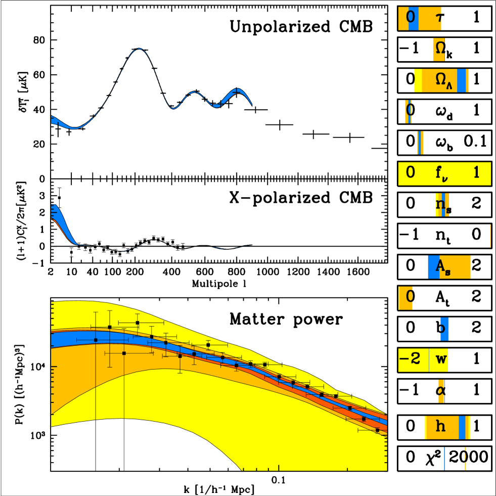
Figure 1: Summary of observations and cosmological models. Data points are for unpolarized CMB experiments combined (top; Appendix A.3 details data used) cross-polarized CMB from WMAP (middle) and Galaxy power from SDSS (bottom). Shaded bands show the 1-sigma range of theoretical models from the Monte-Carlo Markov chains, both for cosmological parameters (right) and for the corresponding power spectra (left). From outside in, these bands correspond to WMAP with no priors, adding the prior $f_{\nu}=0$, $w=-1$, further adding the priors $\Omega_{k}=r=\alpha=0$, and further adding the SDSS information, respectively. These four bands essentially coincide in the top two panels, since the CMB constraints were included in the fits. Note that the $\l$-axis in the upper two panels goes from logarithmic on the left to linear on the right, to show important features at both ends, whereas the $k$-axis of the bottom panel is simply logarithmic.

II Basic Results

Table 1: Cosmological parameters used. Parameters 14-28 are determined by the first 13. Our Monte-Carlo Markov Chain assigns a uniform prior to the parameters labeled “MCMC”. The last six and those labeled “Fits” are closely related to observable power spectrum features Knox03 ; observables ; Kosowsky02 and are helpful for understanding the physical origin of the constraints.

Parameter	Meaning	Status	Use	Definition
$\tau$	Reionization optical depth	Not optional
$\omega_{b}$	Baryon density	Not optional	MCMC	$\omega_{b}=\Omega_{b}h^{2}=\rho_{b}/(1.88\times 10^{-26}$kg$/$m${}^{3})$
$\omega_{d}$	Dark matter density	Not optional	MCMC	$\omega_{d}=\Omega_{d}h^{2}=\rho_{d}/(1.88\times 10^{-26}$kg$/$m${}^{3})$
$f_{\nu}$	Dark matter neutrino fraction	Well motivated	MCMC	$f_{\nu}=\rho_{\nu}/\rho_{d}$
$\Omega_{\Lambda}$	Dark energy density	Not optional	MCMC
$w$	Dark energy equation of state	Worth testing	MCMC	$p_{\Lambda}/\rho_{\Lambda}$ (approximated as constant)
$\Omega_{k}$	Spatial curvature	Worth testing
$A_{s}$	Scalar fluctuation amplitude	Not optional		Primordial scalar power at $k=0.05$/Mpc
${n_{s}}$	Scalar spectral index	Well motivated	MCMC	Primordial spectral index at $k=0.05$/Mpc
$\alpha$	Running of spectral index	Worth testing	MCMC	$\alpha=d\ln{n_{s}}/d\ln k$ (approximated as constant)
$r$	Tensor-to-scalar ratio	Well motivated	MCMC	Tensor-to-scalar power ratio at $k=0.05$/Mpc
${n_{t}}$	Tensor spectral index	Well motivated	MCMC
$b$	Galaxy bias factor	Not optional	MCMC	$b=[P_{\rm galaxy}(k)/P(k)]^{1/2}$ (assumed constant for $k<0.2h/$Mpc)
$z_{\rm ion}$	Reionization redshift (abrupt)			$z_{\rm ion}\approx 92(0.03h\tau/\omega_{b})^{2/3}\Omega_{m}^{1/3}$ (assuming abrupt reionization; reion )
$\omega_{\rm m}$	Physical matter density		Fits	$\omega_{\rm m}=\omega_{b}+\omega_{d}=\Omega_{m}h^{2}$
$\Omega_{m}$	Matter density/critical density			$\Omega_{m}=1-\Omega_{\Lambda}-\Omega_{k}$
$\Omega_{\rm tot}$	Total density/critical density			$\Omega_{\rm tot}=\Omega_{m}+\Omega_{\Lambda}=1-\Omega_{k}$
$A_{t}$	Tensor fluctuation amplitude			$A_{t}=rA_{s}$
$M_{\nu}$	Sum of neutrino masses			$M_{\nu}\approx(94.4\>{\rm eV})\times\omega_{d}f_{\nu}$   KolbTurnerBook
$h$	Hubble parameter			$h=\sqrt{(\omega_{d}+\omega_{b})/(1-\Omega_{k}-\Omega_{\Lambda})}$
$\beta$	Redshift distortion parameter			$\beta\approx[\Omega_{m}^{4/7}+(1+\Omega_{m}/2)(\Omega_{\Lambda}/70)]/b$   Carroll92 ; growl
$t_{0}$	Age of Universe			$t_{0}\approx$($9.785$ Gyr)$\times h^{-1}\int_{0}^{1}[(\Omega_{\Lambda}a^{-(1+3w)}+\Omega_{k}+\Omega_{m}/a)]^{-1/2}da$   KolbTurnerBook
$\sigma_{8}$	Galaxy fluctuation amplitude			$\sigma_{8}=\{4\pi\int_{0}^{\infty}[{3\over x^{3}}(\sin x-x\cos x)]^{2}P(k){k^{2}dk\over(2\pi)^{3}}\}^{1/2}$, $x\equiv k\times 8h^{-1}$Mpc
$Z$	CMB peak suppression factor		MCMC	$Z=e^{-2\tau}$
$A_{p}$	Amplitude on CMB peak scales		MCMC	$A_{p}=A_{s}e^{-2\tau}$
$\Theta_{s}$	Acoustic peak scale (degrees)		MCMC	$\Theta_{s}(\Omega_{k},\Omega_{\Lambda},w,\omega_{d},\omega_{b})$ given by observables
$H_{2}$	2nd to 1st CMB peak ratio		Fits	$H_{2}=(0.925\omega_{\rm m}^{0.18}2.4^{{n_{s}}-1})/[1+(\omega_{b}/0.0164)^{12\omega_{\rm m}^{0.52}})]^{0.2}$   observables
$H_{3}$	3rd to 1st CMB peak ratio		Fits	$H_{3}=2.17[1+(\omega_{b}/0.044)^{2}]^{-1}\omega_{\rm m}^{0.59}3.6^{{n_{s}}-1}/[1+1.63(1-\omega_{b}/0.071)\omega_{\rm m}]$
$A_{*}$	Amplitude at pivot point		Fits	$A_{*}=0.82^{{n_{s}}-1}A_{p}$

II.1 Cosmological parameters

In this paper, we work within the context of a hot Big Bang cosmology with primordial fluctuations that are adiabatic (i.e., we do not allow isocurvature modes) and Gaussian, with negligible generation of fluctuations by cosmic strings, textures, or domain walls. Within this framework, we follow consistent ; Spergel03 in parameterizing our cosmological model in terms of 13 parameters:

$${\bf p}\equiv(\tau,\omega_{b},\omega_{d},f_{\nu},\Omega_{\Lambda},w,\Omega_{k},A_{s},{n_{s}},\alpha,r,{n_{t}},b).$$ (1)

The meaning of these 13 parameters is described in Table 1, together with an additional 16 derived parameters, and their relationship to the original 13.

All parameters are defined just as in version 4.3 of CMBfast cmbfast : in particular, the pivot point unchanged by ${n_{s}}$, $\alpha$ and ${n_{t}}$ is at $0.05$/Mpc, and the tensor normalization convention is such that $r=-8{n_{t}}$ for slow-roll models. $\sigma_{8}$, the linear rms mass fluctuation in spheres of radius $8h^{-1}$Mpc, is determined by the power spectrum, which is in turn determined by ${\bf p}$ via CMBfast. The last six parameters in the table are so-called normal parameters Knox03 , which correspond to observable features in the CMB power spectrum observables ; Kosowsky02 and are useful for having simpler statistical properties than the underlying cosmological parameters as discussed in Appendix A. Since current ${n_{t}}$-constraints are too weak to be interesting, we make the slow-roll assumption ${n_{t}}=-r/8$ throughout this paper rather than treat ${n_{t}}$ as a free parameter.

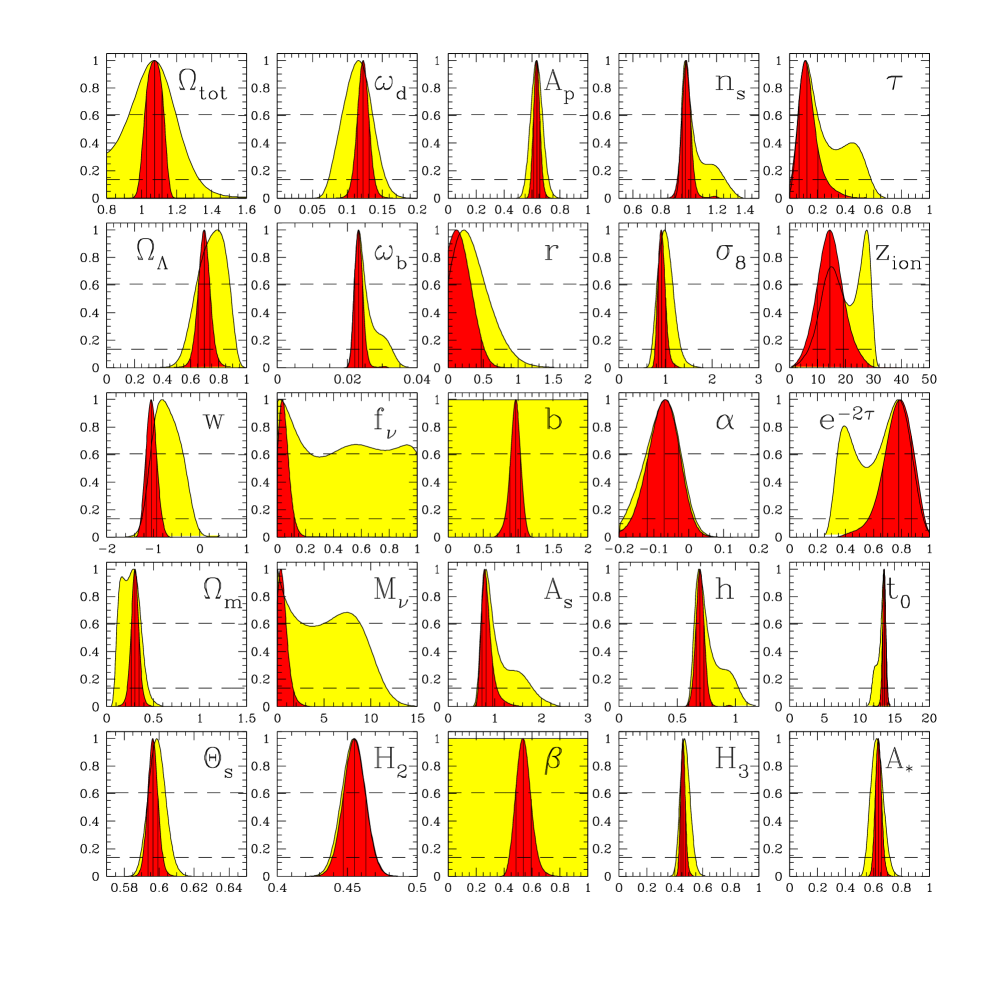
Figure 2: Constraints on individual cosmological quantities using WMAP alone (shaded yellow/light grey distributions) and including SDSS information (narrower red/dark grey distributions). Each distribution shown has been marginalized over all other quantities in the class of 6-parameter $(\tau,\Omega_{\Lambda},\omega_{d},\omega_{b},A_{s},{n_{s}})$ “vanilla” models as well as over a galaxy bias parameter $b$ for the SDSS case. The $\alpha$-distributions are also marginalized over $r$ and $\Omega_{k}$. The parameter measurements and error bars quoted in the tables correspond to the median and the central 68% of the distributions, indicated by three vertical lines for the WMAP+SDSS case above. When the distribution peaks near zero (like for $r$), we instead quote an upper limit at the 95th percentile (single vertical line). The horizontal dashed lines indicate $e^{-x^{2}/2}$ for $x=1$ and $2$, respectively, so if the distribution were Gaussian, its intersections with these lines would correspond to $1\sigma$ and $2\sigma$ limits, respectively.

Table 2: $1\sigma$ constraints on cosmological parameters using WMAP information alone. The columns compare different theoretical priors indicated by numbers in italics. The penultimate column has only the six “vanilla” parameters $(\tau,\Omega_{\Lambda},\omega_{d},\omega_{b},A_{s},{n_{s}})$ free and therefore gives the smallest error bars. The last column uses WMAP temperature data alone, all others also include WMAP polarization information.

	Using WMAP temperature and polarization information						No pol.
	6par$+\Omega_{k}+r+\alpha$	6par+$\Omega_{k}$	6par+$r$	6par+$f_{\nu}$	6par+$w$	6par	6par
$e^{-2\tau}$	$0.52^{+0.21}_{-0.15}$	$0.65^{+0.19}_{-0.32}$	$0.68^{+0.13}_{-0.16}$	$0.75^{+0.12}_{-0.23}$	$0.68^{+0.15}_{-0.21}$	$0.66^{+0.17}_{-0.25}$	$>0.50\>\>(95\%)$
$\Theta_{s}$	$0.602^{+0.010}_{-0.006}$	$0.603^{+0.015}_{-0.005}$	$0.5968^{+0.0048}_{-0.0056}$	$0.5893^{+0.0062}_{-0.0056}$	$0.5966^{+0.0066}_{-0.0105}$	$0.5987^{+0.0052}_{-0.0048}$	$0.5984^{+0.0041}_{-0.0042}$
$\Omega_{\Lambda}$	$0.54^{+0.24}_{-0.33}$	$0.53^{+0.24}_{-0.32}$	$0.823^{+0.058}_{-0.082}$	$0.687^{+0.087}_{-0.097}$	$0.64^{+0.14}_{-0.17}$	$0.75^{+0.10}_{-0.10}$	$0.674^{+0.086}_{-0.093}$
$h^{2}\Omega_{d}$	$0.105^{+0.023}_{-0.023}$	$0.108^{+0.022}_{-0.034}$	$0.097^{+0.021}_{-0.018}$	$0.119^{+0.018}_{-0.016}$	$0.118^{+0.020}_{-0.020}$	$0.115^{+0.020}_{-0.021}$	$0.129^{+0.019}_{-0.018}$
$h^{2}\Omega_{b}$	$0.0238^{+0.0035}_{-0.0027}$	$0.0241^{+0.0055}_{-0.0020}$	$0.0256^{+0.0025}_{-0.0019}$	$0.0247^{+0.0029}_{-0.0016}$	$0.0246^{+0.0038}_{-0.0017}$	$0.0245^{+0.0050}_{-0.0019}$	$0.0237^{+0.0018}_{-0.0013}$
$f_{\nu}$	${\it 0}$	${\it 0}$	${\it 0}$	No constraint	${\it 0}$	${\it 0}$	${\it 0}$
$n_{s}$	$0.97^{+0.13}_{-0.10}$	$1.01^{+0.18}_{-0.06}$	$1.064^{+0.066}_{-0.059}$	$0.962^{+0.098}_{-0.041}$	$1.03^{+0.12}_{-0.05}$	$1.02^{+0.16}_{-0.06}$	$0.989^{+0.061}_{-0.031}$
$n_{t}+1$	$0.9847^{+0.0097}_{-0.0141}$	${\it 1}$	$0.959^{+0.026}_{-0.037}$	${\it 1}$	${\it 1}$	${\it 1}$	${\it 1}$
$A_{p}$	$0.593^{+0.053}_{-0.044}$	$0.602^{+0.053}_{-0.051}$	$0.592^{+0.049}_{-0.046}$	$0.602^{+0.045}_{-0.050}$	$0.637^{+0.045}_{-0.046}$	$0.633^{+0.044}_{-0.041}$	$0.652^{+0.049}_{-0.046}$
$r$	$<0.90\>\>(95\%)$	${\it 0}$	$<0.84\>\>(95\%)$	${\it 0}$	${\it 0}$	${\it 0}$	${\it 0}$
$b$	No constraint	No constraint	No constraint	No constraint	No constraint	No constraint	No constraint
$w$	${\it-1}$	${\it-1}$	${\it-1}$	${\it-1}$	$-0.72^{+0.34}_{-0.27}$	${\it-1}$	${\it-1}$
$\alpha$	$-0.075^{+0.047}_{-0.055}$	${\it 0}$	${\it 0}$	${\it 0}$	${\it 0}$	${\it 0}$	${\it 0}$
$\Omega_{\rm tot}$	$1.095^{+0.094}_{-0.144}$	$1.086^{+0.057}_{-0.128}$	${\it 0}$	${\it 0}$	${\it 0}$	${\it 0}$	${\it 0}$
$\Omega_{m}$	$0.57^{+0.45}_{-0.33}$	$0.55^{+0.47}_{-0.29}$	$0.177^{+0.082}_{-0.058}$	$0.313^{+0.097}_{-0.087}$	$0.36^{+0.17}_{-0.14}$	$0.25^{+0.10}_{-0.10}$	$0.326^{+0.093}_{-0.086}$
$h^{2}\Omega_{m}$	$0.128^{+0.022}_{-0.021}$	$0.132^{+0.021}_{-0.028}$	$0.123^{+0.020}_{-0.018}$	$0.144^{+0.018}_{-0.016}$	$0.143^{+0.020}_{-0.019}$	$0.140^{+0.020}_{-0.018}$	$0.153^{+0.020}_{-0.018}$
$h$	$0.48^{+0.27}_{-0.12}$	$0.50^{+0.16}_{-0.13}$	$0.84^{+0.12}_{-0.10}$	$0.674^{+0.087}_{-0.049}$	$0.63^{+0.14}_{-0.10}$	$0.74^{+0.18}_{-0.07}$	$0.684^{+0.070}_{-0.045}$
$\tau$	$0.33^{+0.17}_{-0.17}$	$0.22^{+0.34}_{-0.13}$	$0.19^{+0.13}_{-0.09}$	$0.15^{+0.18}_{-0.07}$	$0.19^{+0.18}_{-0.10}$	$0.21^{+0.24}_{-0.11}$	$<0.35\>\>(95\%)$
$z_{ion}$	$25.9^{+4.4}_{-8.8}$	$20.1^{+9.2}_{-8.3}$	$17.1^{+5.8}_{-5.8}$	$15.5^{+8.6}_{-5.6}$	$18.5^{+7.1}_{-6.6}$	$19.6^{+7.8}_{-7.4}$	$<25\>\>(95\%)$
$A_{s}$	$1.14^{+0.42}_{-0.31}$	$0.97^{+0.73}_{-0.23}$	$0.87^{+0.28}_{-0.16}$	$0.81^{+0.35}_{-0.13}$	$0.94^{+0.40}_{-0.18}$	$0.98^{+0.56}_{-0.21}$	$0.80^{+0.26}_{-0.12}$
$A_{t}$	$0.14^{+0.13}_{-0.10}$	${\it 0}$	$0.30^{+0.22}_{-0.17}$	${\it 0}$	${\it 0}$	${\it 0}$	${\it 0}$
$\beta$	No constraint	No constraint	No constraint	No constraint	No constraint	No constraint	No constraint
$t_{0}[$Gyr$]$	$16.5^{+2.6}_{-3.1}$	$16.3^{+2.3}_{-1.8}$	$13.00^{+0.41}_{-0.47}$	$13.75^{+0.36}_{-0.59}$	$13.53^{+0.52}_{-0.65}$	$13.24^{+0.41}_{-0.89}$	$13.41^{+0.29}_{-0.37}$
$\sigma_{8}$	$0.90^{+0.13}_{-0.13}$	$0.87^{+0.15}_{-0.13}$	$0.84^{+0.17}_{-0.17}$	$0.32^{+0.36}_{-0.32}$	$0.95^{+0.16}_{-0.14}$	$0.99^{+0.19}_{-0.14}$	$0.94^{+0.15}_{-0.12}$
$H_{2}$	$0.441^{+0.013}_{-0.014}$	$0.4581^{+0.0090}_{-0.0083}$	$0.4541^{+0.0067}_{-0.0081}$	$0.426^{+0.018}_{-0.010}$	$0.4541^{+0.0084}_{-0.0085}$	$0.4543^{+0.0083}_{-0.0085}$	$0.4541^{+0.0085}_{-0.0086}$
$H_{3}$	$0.424^{+0.043}_{-0.040}$	$0.455^{+0.033}_{-0.029}$	$0.452^{+0.034}_{-0.033}$	$0.441^{+0.039}_{-0.033}$	$0.477^{+0.036}_{-0.034}$	$0.474^{+0.037}_{-0.033}$	$0.475^{+0.032}_{-0.030}$
$A_{*}$	$0.595^{+0.056}_{-0.048}$	$0.599^{+0.055}_{-0.064}$	$0.584^{+0.050}_{-0.046}$	$0.602^{+0.045}_{-0.046}$	$0.631^{+0.047}_{-0.045}$	$0.624^{+0.048}_{-0.042}$	$0.652^{+0.048}_{-0.046}$
$M_{\nu}[$eV$]$	${\it 0}$	${\it 0}$	${\it 0}$	$<10.6\>\>(95\%)$	${\it 0}$	${\it 0}$	${\it 0}$
$\chi^{2}$/dof	$1426.1/1339$	$1428.4/1341$	$1430.9/1341$	$1431.8/1341$	$1431.8/1341$	$1431.5/1342$	$972.4/893$

Table 3: $1\sigma$ constraints on cosmological parameters combining CMB and SDSS information. The columns compare different theoretical priors indicated by italics. The second last column drops the polarized WMAP information and the last column drops all WMAP information, replacing it by pre-WMAP CMB experiments. The 6par$+w$ column includes SN Ia information.

	Using SDSS + WMAP temperature and polarization information						No pol.	No WMAP
	6par$+\Omega_{k}+r+\alpha$	6par+$\Omega_{k}$	6par+$r$	6par+$f_{\nu}$	6par+$w$	6par	6par	6par
$e^{-2\tau}$	$0.53^{+0.22}_{-0.17}$	$0.69^{+0.15}_{-0.32}$	$0.776^{+0.098}_{-0.116}$	$0.776^{+0.095}_{-0.121}$	$0.80^{+0.10}_{-0.13}$	$0.780^{+0.094}_{-0.119}$	$>0.63\>\>(95\%)$	$>0.71\>\>(95\%)$
$\Theta_{s}$	$0.601^{+0.010}_{-0.006}$	$0.600^{+0.013}_{-0.004}$	$0.5982^{+0.0034}_{-0.0032}$	$0.5948^{+0.0033}_{-0.0030}$	$0.5954^{+0.0037}_{-0.0038}$	$0.5965^{+0.0031}_{-0.0030}$	$0.5968^{+0.0030}_{-0.0030}$	$0.5977^{+0.0048}_{-0.0045}$
$\Omega_{\Lambda}$	$0.660^{+0.080}_{-0.097}$	$0.653^{+0.082}_{-0.084}$	$0.727^{+0.041}_{-0.042}$	$0.620^{+0.074}_{-0.087}$	$0.706^{+0.032}_{-0.033}$	$0.699^{+0.042}_{-0.045}$	$0.684^{+0.041}_{-0.046}$	$0.691^{+0.039}_{-0.053}$
$h^{2}\Omega_{d}$	$0.103^{+0.020}_{-0.022}$	$0.103^{+0.016}_{-0.024}$	$0.1195^{+0.0084}_{-0.0082}$	$0.135^{+0.014}_{-0.012}$	$0.124^{+0.012}_{-0.011}$	$0.1222^{+0.0090}_{-0.0082}$	$0.1254^{+0.0093}_{-0.0083}$	$0.1252^{+0.0088}_{-0.0076}$
$h^{2}\Omega_{b}$	$0.0238^{+0.0036}_{-0.0026}$	$0.0232^{+0.0051}_{-0.0017}$	$0.0242^{+0.0017}_{-0.0013}$	$0.0234^{+0.0014}_{-0.0011}$	$0.0232^{+0.0013}_{-0.0010}$	$0.0232^{+0.0013}_{-0.0010}$	$0.0231^{+0.0011}_{-0.0009}$	$0.0229^{+0.0016}_{-0.0015}$
$f_{\nu}$	${\it 0}$	${\it 0}$	${\it 0}$	$<0.12\>\>(95\%)$	${\it 0}$	${\it 0}$	${\it 0}$	${\it 0}$
$n_{s}$	$0.97^{+0.12}_{-0.10}$	$0.98^{+0.18}_{-0.04}$	$1.012^{+0.049}_{-0.036}$	$0.972^{+0.041}_{-0.027}$	$0.976^{+0.040}_{-0.024}$	$0.977^{+0.039}_{-0.025}$	$0.973^{+0.030}_{-0.021}$	$1.015^{+0.036}_{-0.033}$
$n_{t}+1$	$0.9852^{+0.0093}_{-0.0154}$	${\it 1}$	$0.976^{+0.016}_{-0.021}$	${\it 1}$	${\it 1}$	${\it 1}$	${\it 1}$	${\it 1}$
$A_{p}$	$0.584^{+0.045}_{-0.033}$	$0.584^{+0.038}_{-0.028}$	$0.635^{+0.023}_{-0.021}$	$0.645^{+0.029}_{-0.026}$	$0.637^{+0.027}_{-0.027}$	$0.633^{+0.024}_{-0.022}$	$0.637^{+0.025}_{-0.023}$	$0.588^{+0.025}_{-0.025}$
$r$	$<0.50\>\>(95\%)$	${\it 0}$	$<0.47\>\>(95\%)$	${\it 0}$	${\it 0}$	${\it 0}$	${\it 0}$	${\it 0}$
$b$	$0.94^{+0.12}_{-0.10}$	$1.03^{+0.15}_{-0.13}$	$0.963^{+0.075}_{-0.081}$	$1.061^{+0.096}_{-0.105}$	$0.956^{+0.075}_{-0.076}$	$0.962^{+0.073}_{-0.083}$	$1.009^{+0.068}_{-0.091}$	$1.068^{+0.066}_{-0.079}$
$w$	${\it-1}$	${\it-1}$	${\it-1}$	${\it-1}$	$-1.05^{+0.13}_{-0.14}$	${\it-1}$	${\it-1}$	${\it-1}$
$\alpha$	$-0.071^{+0.042}_{-0.047}$	${\it 0}$	${\it 0}$	${\it 0}$	${\it 0}$	${\it 0}$	${\it 0}$	${\it 0}$
$\Omega_{\rm tot}$	$1.056^{+0.045}_{-0.045}$	$1.058^{+0.039}_{-0.041}$	${\it 0}$	${\it 0}$	${\it 0}$	${\it 0}$	${\it 0}$	${\it 0}$
$\Omega_{m}$	$0.40^{+0.10}_{-0.09}$	$0.406^{+0.093}_{-0.091}$	$0.273^{+0.042}_{-0.041}$	$0.380^{+0.087}_{-0.074}$	$0.294^{+0.033}_{-0.032}$	$0.301^{+0.045}_{-0.042}$	$0.316^{+0.046}_{-0.041}$	$0.309^{+0.053}_{-0.039}$
$h^{2}\Omega_{m}$	$0.126^{+0.019}_{-0.019}$	$0.126^{+0.016}_{-0.019}$	$0.1438^{+0.0084}_{-0.0080}$	$0.158^{+0.015}_{-0.012}$	$0.147^{+0.012}_{-0.011}$	$0.1454^{+0.0091}_{-0.0082}$	$0.1486^{+0.0095}_{-0.0084}$	$0.1481^{+0.0091}_{-0.0077}$
$h$	$0.55^{+0.11}_{-0.06}$	$0.550^{+0.092}_{-0.055}$	$0.725^{+0.049}_{-0.036}$	$0.645^{+0.048}_{-0.040}$	$0.708^{+0.033}_{-0.030}$	$0.695^{+0.039}_{-0.031}$	$0.685^{+0.033}_{-0.028}$	$0.693^{+0.038}_{-0.040}$
$\tau$	$0.32^{+0.19}_{-0.17}$	$0.18^{+0.31}_{-0.10}$	$0.127^{+0.081}_{-0.059}$	$0.127^{+0.085}_{-0.058}$	$0.113^{+0.090}_{-0.059}$	$0.124^{+0.083}_{-0.057}$	$<0.23\>\>(95\%)$	$<0.17\>\>(95\%)$
$z_{ion}$	$25.3^{+4.8}_{-8.8}$	$18^{+10}_{-7}$	$14.1^{+4.8}_{-4.7}$	$14.9^{+5.4}_{-4.8}$	$13.6^{+5.7}_{-5.2}$	$14.4^{+5.2}_{-4.7}$	$<20\>\>(95\%)$	$<18\>\>(95\%)$
$A_{s}$	$1.12^{+0.43}_{-0.31}$	$0.86^{+0.68}_{-0.16}$	$0.82^{+0.15}_{-0.10}$	$0.83^{+0.16}_{-0.09}$	$0.80^{+0.15}_{-0.09}$	$0.81^{+0.15}_{-0.09}$	$0.72^{+0.15}_{-0.07}$	$0.64^{+0.10}_{-0.04}$
$A_{t}$	$0.14^{+0.12}_{-0.09}$	${\it 0}$	$0.16^{+0.15}_{-0.11}$	${\it 0}$	${\it 0}$	${\it 0}$	${\it 0}$	${\it 0}$
$\beta$	$0.633^{+0.081}_{-0.076}$	$0.587^{+0.066}_{-0.062}$	$0.506^{+0.056}_{-0.053}$	$0.554^{+0.059}_{-0.054}$	$0.533^{+0.051}_{-0.048}$	$0.537^{+0.056}_{-0.052}$	$0.529^{+0.059}_{-0.052}$	$0.493^{+0.060}_{-0.051}$
$t_{0}[$Gyr$]$	$15.8^{+1.5}_{-1.8}$	$15.9^{+1.3}_{-1.5}$	$13.32^{+0.27}_{-0.33}$	$13.65^{+0.25}_{-0.28}$	$13.47^{+0.26}_{-0.27}$	$13.54^{+0.23}_{-0.27}$	$13.55^{+0.21}_{-0.23}$	$13.51^{+0.32}_{-0.31}$
$\sigma_{8}$	$0.91^{+0.11}_{-0.10}$	$0.86^{+0.13}_{-0.11}$	$0.919^{+0.086}_{-0.073}$	$0.823^{+0.098}_{-0.077}$	$0.928^{+0.084}_{-0.076}$	$0.917^{+0.090}_{-0.072}$	$0.879^{+0.088}_{-0.062}$	$0.842^{+0.069}_{-0.053}$
$H_{2}$	$0.441^{+0.013}_{-0.012}$	$0.4577^{+0.0086}_{-0.0082}$	$0.4535^{+0.0081}_{-0.0084}$	$0.4521^{+0.0091}_{-0.0100}$	$0.4545^{+0.0087}_{-0.0090}$	$0.4550^{+0.0083}_{-0.0082}$	$0.4549^{+0.0082}_{-0.0083}$	$0.475^{+0.018}_{-0.020}$
$H_{3}$	$0.422^{+0.027}_{-0.031}$	$0.444^{+0.026}_{-0.025}$	$0.468^{+0.019}_{-0.017}$	$0.472^{+0.022}_{-0.019}$	$0.461^{+0.018}_{-0.017}$	$0.459^{+0.018}_{-0.016}$	$0.460^{+0.017}_{-0.015}$	$0.485^{+0.020}_{-0.018}$
$A_{*}$	$0.587^{+0.049}_{-0.041}$	$0.582^{+0.041}_{-0.036}$	$0.632^{+0.022}_{-0.021}$	$0.648^{+0.028}_{-0.025}$	$0.639^{+0.027}_{-0.028}$	$0.635^{+0.024}_{-0.022}$	$0.639^{+0.024}_{-0.022}$	$0.586^{+0.024}_{-0.025}$
$M_{\nu}[$eV$]$	${\it 0}$	${\it 0}$	${\it 0}$	$<1.74\>\>(95\%)$	${\it 0}$	${\it 0}$	${\it 0}$	${\it 0}$
$\chi^{2}$/dof	$1444.4/1357$	$1445.4/1359$	$1446.9/1359$	$1447.3/1359$	$1622.0/1531$	$1447.2/1360$	$987.8/911$	$134.6/163$

Table 4: $1\sigma$ constraints on cosmological parameters as progressively more information/assumptions are added. First column uses WMAP data alone and treats the 9 parameters $(\tau,\Omega_{k},\Omega_{\Lambda},\omega_{d},\omega_{b},A_{s},{n_{s}},\alpha,r)$ as unknown, so the only assumptions are $f_{\nu}=0$, $w=-1$. Moving to the right in the table, we add the assumptions $r=\alpha=0$, then add SDSS information, then add SN Ia information, then add the assumption that $\tau<0.3$. The next two columns are for 6-parameter vanilla models $(\Omega_{k}=r=\alpha=0)$, first using WMAP+SDSS data alone, then adding small-scale non-WMAP CMB data. The last two columns use WMAP+SDSS alone for 5-parameter models assuming ${n_{s}}=1$ (“vanilla lite”) and ${n_{s}}=0.96$, $r=0.15$ ($V\propto\phi^{2}$ stochastic eternal inflation), respectively.

	9 parameters $(\tau,\Omega_{k},\Omega_{\Lambda},\omega_{d},\omega_{b},A_{s},{n_{s}},\alpha,r)$ free					WMAP+SDSS, 6 vanilla parameters free
	WMAP	$+r=\alpha=0$	$+$SDSS	$+$SN Ia	$+\tau<0.3$		$+$other CMB	$+{n_{s}}=1$	$+V(\phi)\propto\phi^{2}$
$e^{-2\tau}$	$0.52^{+0.21}_{-0.15}$	$0.65^{+0.19}_{-0.32}$	$0.69^{+0.15}_{-0.32}$	$0.44^{+0.34}_{-0.13}$	$0.75^{+0.11}_{-0.12}$	$0.780^{+0.094}_{-0.119}$	$0.813^{+0.081}_{-0.092}$	$0.720^{+0.057}_{-0.049}$	$0.833^{+0.063}_{-0.059}$
$\Theta_{s}$	$0.602^{+0.010}_{-0.006}$	$0.603^{+0.015}_{-0.005}$	$0.600^{+0.013}_{-0.004}$	$0.606^{+0.011}_{-0.010}$	$0.5971^{+0.0034}_{-0.0034}$	$0.5965^{+0.0031}_{-0.0030}$	$0.5956^{+0.0025}_{-0.0026}$	$0.5979^{+0.0024}_{-0.0024}$	$0.5953^{+0.0021}_{-0.0022}$
$\Omega_{\Lambda}$	$0.54^{+0.24}_{-0.33}$	$0.53^{+0.24}_{-0.32}$	$0.653^{+0.082}_{-0.084}$	$0.725^{+0.039}_{-0.044}$	$0.695^{+0.034}_{-0.037}$	$0.699^{+0.042}_{-0.045}$	$0.691^{+0.032}_{-0.040}$	$0.707^{+0.031}_{-0.039}$	$0.685^{+0.032}_{-0.041}$
$h^{2}\Omega_{d}$	$0.105^{+0.023}_{-0.023}$	$0.108^{+0.022}_{-0.034}$	$0.103^{+0.016}_{-0.024}$	$0.090^{+0.028}_{-0.016}$	$0.115^{+0.012}_{-0.012}$	$0.1222^{+0.0090}_{-0.0082}$	$0.1231^{+0.0075}_{-0.0068}$	$0.1233^{+0.0089}_{-0.0079}$	$0.1233^{+0.0082}_{-0.0071}$
$h^{2}\Omega_{b}$	$0.0238^{+0.0035}_{-0.0027}$	$0.0241^{+0.0055}_{-0.0020}$	$0.0232^{+0.0051}_{-0.0017}$	$0.0263^{+0.0042}_{-0.0036}$	$0.0230^{+0.0013}_{-0.0011}$	$0.0232^{+0.0013}_{-0.0010}$	$0.0228^{+0.0010}_{-0.0008}$	$0.0238^{+0.0006}_{-0.0006}$	$0.0226^{+0.0006}_{-0.0006}$
$f_{\nu}$	${\it 0}$	${\it 0}$	${\it 0}$	${\it 0}$	${\it 0}$	${\it 0}$	${\it 0}$	${\it 0}$	${\it 0}$
$n_{s}$	$0.97^{+0.13}_{-0.10}$	$1.01^{+0.18}_{-0.06}$	$0.98^{+0.18}_{-0.04}$	$1.10^{+0.11}_{-0.13}$	$0.979^{+0.036}_{-0.029}$	$0.977^{+0.039}_{-0.025}$	$0.966^{+0.025}_{-0.020}$	${\it 1}$	${\it 0.96}$
$n_{t}+1$	$0.9847^{+0.0097}_{-0.0141}$	${\it 1}$	${\it 1}$	${\it 1}$	${\it 1}$	${\it 1}$	${\it 1}$	${\it 1}$	${\it 0.993}$
$A_{p}$	$0.593^{+0.053}_{-0.044}$	$0.602^{+0.053}_{-0.051}$	$0.584^{+0.038}_{-0.028}$	$0.582^{+0.043}_{-0.025}$	$0.613^{+0.034}_{-0.033}$	$0.633^{+0.024}_{-0.022}$	$0.631^{+0.020}_{-0.019}$	$0.642^{+0.023}_{-0.022}$	$0.629^{+0.021}_{-0.019}$
$r$	$<0.50\>\>(95\%)$	${\it 0}$	${\it 0}$	${\it 0}$	${\it 0}$	${\it 0}$	${\it 0}$	${\it 0}$	${\it 0.15}$
$b$	${\it 1}$	${\it 1}$	$1.03^{+0.15}_{-0.13}$	$0.93^{+0.10}_{-0.08}$	$0.998^{+0.098}_{-0.088}$	$0.962^{+0.073}_{-0.083}$	$0.990^{+0.060}_{-0.062}$	$0.918^{+0.036}_{-0.033}$	$1.006^{+0.043}_{-0.039}$
$w$	${\it-1}$	${\it-1}$	${\it-1}$	${\it-1}$	${\it-1}$	${\it-1}$	${\it-1}$	${\it-1}$	${\it-1}$
$\alpha$	$-0.075^{+0.047}_{-0.055}$	${\it 0}$	${\it 0}$	${\it 0}$	${\it 0}$	${\it 0}$	${\it 0}$	${\it 0}$	${\it 0}$
$\Omega_{\rm tot}$	$1.095^{+0.094}_{-0.144}$	$1.086^{+0.057}_{-0.128}$	$1.058^{+0.039}_{-0.041}$	$1.054^{+0.048}_{-0.041}$	$1.012^{+0.018}_{-0.022}$	${\it 0}$	${\it 0}$	${\it 0}$	${\it 0}$
$\Omega_{m}$	$0.57^{+0.45}_{-0.33}$	$0.55^{+0.47}_{-0.29}$	$0.406^{+0.093}_{-0.091}$	$0.328^{+0.050}_{-0.049}$	$0.317^{+0.053}_{-0.045}$	$0.301^{+0.045}_{-0.042}$	$0.309^{+0.040}_{-0.032}$	$0.293^{+0.039}_{-0.031}$	$0.315^{+0.041}_{-0.032}$
$h^{2}\Omega_{m}$	$0.128^{+0.022}_{-0.021}$	$0.132^{+0.021}_{-0.028}$	$0.126^{+0.016}_{-0.019}$	$0.117^{+0.024}_{-0.013}$	$0.138^{+0.012}_{-0.012}$	$0.1454^{+0.0091}_{-0.0082}$	$0.1459^{+0.0077}_{-0.0071}$	$0.1471^{+0.0090}_{-0.0080}$	$0.1459^{+0.0084}_{-0.0073}$
$h$	$0.48^{+0.27}_{-0.12}$	$0.50^{+0.16}_{-0.13}$	$0.550^{+0.092}_{-0.055}$	$0.599^{+0.090}_{-0.062}$	$0.660^{+0.067}_{-0.064}$	$0.695^{+0.039}_{-0.031}$	$0.685^{+0.027}_{-0.026}$	$0.708^{+0.023}_{-0.024}$	$0.680^{+0.022}_{-0.024}$
$\tau$	$0.33^{+0.17}_{-0.17}$	$0.22^{+0.34}_{-0.13}$	$0.18^{+0.31}_{-0.10}$	$0.41^{+0.17}_{-0.28}$	$0.143^{+0.089}_{-0.066}$	$0.124^{+0.083}_{-0.057}$	$0.103^{+0.060}_{-0.047}$	$0.165^{+0.035}_{-0.038}$	$0.092^{+0.036}_{-0.036}$
$z_{ion}$	$25.9^{+4.4}_{-8.8}$	$20.1^{+9.2}_{-8.3}$	$18^{+10}_{-7}$	$26.7^{+3.2}_{-12.4}$	$15.6^{+5.1}_{-5.0}$	$14.4^{+5.2}_{-4.7}$	$12.8^{+4.3}_{-4.2}$	$17.0^{+2.2}_{-2.6}$	$11.9^{+2.9}_{-3.4}$
$A_{s}$	$1.14^{+0.42}_{-0.31}$	$0.97^{+0.73}_{-0.23}$	$0.86^{+0.68}_{-0.16}$	$1.30^{+0.50}_{-0.51}$	$0.82^{+0.14}_{-0.11}$	$0.81^{+0.15}_{-0.09}$	$0.777^{+0.100}_{-0.072}$	$0.893^{+0.051}_{-0.053}$	$0.758^{+0.050}_{-0.050}$
$A_{t}$	$0.14^{+0.13}_{-0.10}$	${\it 0}$	${\it 0}$	${\it 0}$	${\it 0}$	${\it 0}$	${\it 0}$	${\it 0}$	$0.1137^{+0.0075}_{-0.0074}$
$\beta$	$0.73^{+0.28}_{-0.29}$	$0.72^{+0.29}_{-0.24}$	$0.587^{+0.066}_{-0.062}$	$0.577^{+0.062}_{-0.063}$	$0.530^{+0.050}_{-0.045}$	$0.537^{+0.056}_{-0.052}$	$0.534^{+0.044}_{-0.046}$	$0.553^{+0.054}_{-0.047}$	$0.525^{+0.052}_{-0.045}$
$t_{0}[$Gyr$]$	$16.5^{+2.6}_{-3.1}$	$16.3^{+2.3}_{-1.8}$	$15.9^{+1.3}_{-1.5}$	$15.6^{+1.4}_{-1.8}$	$14.1^{+1.0}_{-0.9}$	$13.54^{+0.23}_{-0.27}$	$13.62^{+0.20}_{-0.20}$	$13.40^{+0.13}_{-0.12}$	$13.67^{+0.12}_{-0.12}$
$\sigma_{8}$	$0.90^{+0.13}_{-0.13}$	$0.87^{+0.15}_{-0.13}$	$0.86^{+0.13}_{-0.11}$	$0.948^{+0.089}_{-0.101}$	$0.882^{+0.094}_{-0.084}$	$0.917^{+0.090}_{-0.072}$	$0.894^{+0.060}_{-0.055}$	$0.966^{+0.046}_{-0.050}$	$0.879^{+0.041}_{-0.046}$
$H_{2}$	$0.441^{+0.013}_{-0.014}$	$0.4581^{+0.0090}_{-0.0083}$	$0.4577^{+0.0086}_{-0.0082}$	$0.4585^{+0.0086}_{-0.0093}$	$0.4558^{+0.0082}_{-0.0083}$	$0.4550^{+0.0083}_{-0.0082}$	$0.4552^{+0.0087}_{-0.0079}$	$0.4543^{+0.0081}_{-0.0081}$	$0.4556^{+0.0081}_{-0.0081}$
$H_{3}$	$0.424^{+0.043}_{-0.040}$	$0.455^{+0.033}_{-0.029}$	$0.444^{+0.026}_{-0.025}$	$0.457^{+0.020}_{-0.021}$	$0.449^{+0.021}_{-0.021}$	$0.459^{+0.018}_{-0.016}$	$0.454^{+0.013}_{-0.012}$	$0.467^{+0.012}_{-0.011}$	$0.451^{+0.011}_{-0.010}$
$A_{*}$	$0.595^{+0.056}_{-0.048}$	$0.599^{+0.055}_{-0.064}$	$0.582^{+0.041}_{-0.036}$	$0.567^{+0.058}_{-0.028}$	$0.616^{+0.033}_{-0.032}$	$0.635^{+0.024}_{-0.022}$	$0.634^{+0.020}_{-0.018}$	$0.642^{+0.023}_{-0.022}$	$0.634^{+0.021}_{-0.019}$
$M_{\nu}[$eV$]$	${\it 0}$	${\it 0}$	${\it 0}$	${\it 0}$	${\it 0}$	${\it 0}$	${\it 0}$	${\it 0}$	${\it 0}$
$\chi^{2}/$dof	$1426.1/1339$	$1428.4/1341$	$1445.4/1359$	$1619.6/1530$	$1621.8/1530$	$1447.2/1360$	$1475.6/1395$	$1447.9/1359$	$1447.1/1395$

II.2 Constraints

We constrain theoretical models using the Monte Carlo Markov Chain method Metropolis ; Hastings ; Gilks96 ; GelmanRubin92 ; Christensen01 ; Lewis02 ; Slosar03 implemented as described in Appendix A. Unless otherwise stated, we use the WMAP temperature and cross-polarization power spectra Bennett03 ; Hinshaw03 ; kogut03 ; Page3-03 , evaluating likelihoods with the software provided by the WMAP team Verde03 . When using SDSS information, we fit the nonlinear theoretical power spectrum $P(k)$ approximation of Smith03 to the observations reported by the SDSS team sdsspower , assuming an unknown scale-independent linear bias $b$ to be marginalized over. This means that we use only the shape of the measured SDSS power spectrum, not its amplitude. We use only the measurements with $k\leq 0.2h/{\rm Mpc}$ as suggested by sdsspower . The WMAP team used this same $k$-limit when analyzing the 2dFGRS Verde03 ; we show in Section VIII.3 that cutting back to $k\leq 0.15h/{\rm Mpc}$ causes a negligible change in our best-fit model. To be conservative, we do not use the SDSS measurement of redshift space distortion parameter $\beta$ sdsspower , nor do we use any other information (“priors”) whatsoever unless explicitly stated. When using SN Ia information, we employ the 172 SN Ia redshifts and corrected magnitudes compiled and uniformly analyzed by Tonry et al. Tonry03 , evaluating the likelihood with the software provided by their team, which marginalizes over the corrected SN Ia “standard candle” absolute magnitude. Note that this is an updated and expanded data set from that available to the WMAP team when they carried out their analysisSpergel03 .

Our constraints on individual cosmological parameters are given in Tables 2-4 and illustrated in Figure 2, both for WMAP alone and when including additional information such as that from the SDSS. To avoid losing sight of the forest for all the threes (and other digits), we will spend most of the remainder of this paper digesting this voluminous information one step at a time, focusing on what WMAP and SDSS do and don’t tell us about the underlying physics. The one-dimensional constraints in the tables and Figure 2 fail to reveal important information hidden in parameter correlations and degeneracies, so a powerful tool will be studying the joint constraints on key 2-parameter pairs. We will begin with a simple 6-parameter space of models, then gradually introduce additional parameters to quantify both how accurately we can measure them and to what extent they weaken the constraints on the other parameters.

III Vanilla $\Lambda$CDM models

In this section, we explore constraints on six-parameter “vanilla” models that have no spatial curvature ($\Omega_{k}=0$), no gravity waves ($r=0$), no running tilt ($\alpha=0$), negligible neutrino masses ($f_{\nu}=0$) and dark energy corresponding to a pure cosmological constant ($w=-1$). These vanilla $\Lambda$CDM models are thus determined by merely six parameters: the matter budget ($\Omega_{\Lambda},\omega_{d},\omega_{b}$), the initial conditions ($A_{s},{n_{s}}$) and the reionization optical depth $\tau$. (When including SDSS information, we bring in the bias parameter $b$ as well.)

Our constraints on individual cosmological parameters are shown in Tables 2-4 and Figure 2 both for WMAP alone and when including SDSS information. Several features are noteworthy.

First of all, as emphasized by the WMAP team Spergel03 , error bars have shrunk dramatically compared to the situation before WMAP, and it is therefore quite impressive that any vanilla model is still able to fit both the unpolarized and polarized CMB data. The best fit model (Table 2) has $\chi^{2}\sim 1431.5$ for $899+449-6=1342$ effective degrees of freedom, i.e., about $1.7\sigma$ high if taken at face value. The WMAP team provide an extensive discussion of possible origins of this slight excess, and argue that it comes mainly from three unexplained “blips” Verde03 ; Lewis03 , deviations from the model fit over a narrow range of $\l$, in the measured temperature power spectrum. They argue that these blips have nothing to do with features in any standard cosmological models, since adding the above-mentioned non-vanilla parameters does not reduce $\chi^{2}$ substantially — we confirm this below, and will not dwell further on these sharp features. Adding the 19 SDSS data points increases the effective degrees of freedom by $19-1=18$ (since this requires the addition of the bias parameter $b$), yet raises the best-fit $\chi^{2}$ by only $15.7$. Indeed, Figure 1 shows that even the model best fitting WMAP alone does a fine job at fitting the SDSS data with no further parameter tuning.

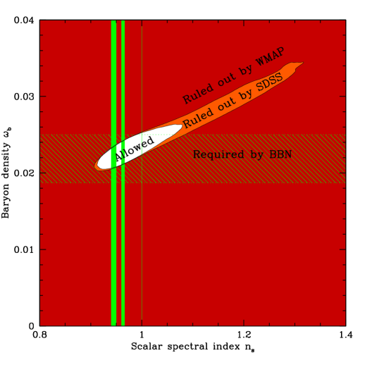
Figure 3: 95% constraints in the $({n_{s}},\omega_{b})$ plane. The shaded dark red/grey region is ruled out by WMAP alone for 6-parameter “vanilla” models, leaving the long degeneracy banana discussed in the text. The shaded light red/grey region is ruled out when adding SDSS information. The hatched band is required by Big Bang Nucleosynthesis (BBN). From right to left, the three vertical bands correspond to a scale-invariant Harrison-Zel’dovich spectrum and to the common inflationary predictions ${n_{s}}=1-2/N\sim 0.96$ and ${n_{s}}=1-3/N\sim 0.94$ (Table 6), assuming that the number of e-foldings between horizon exit of the observed fluctuations and the end of inflation is $50<N<60$.

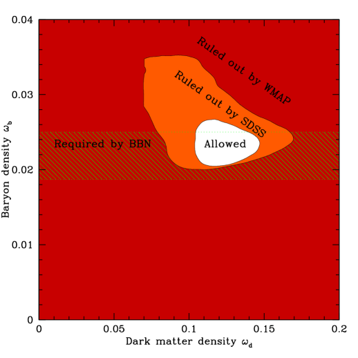
Figure 4: 95% constraints in the $(\omega_{d},\omega_{b})$ plane. Shaded dark red/grey region is ruled out by WMAP alone for 6-parameter “vanilla” models. The shaded light red/grey region is ruled out when adding SDSS information. The hatched band is required by Big Bang Nucleosynthesis (BBN).

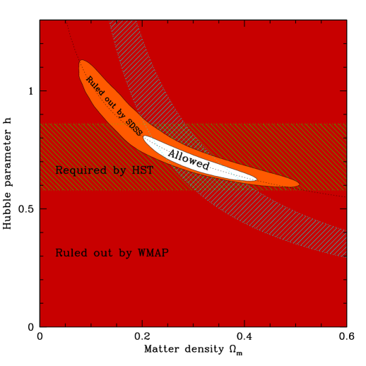
Figure 5: 95% constraints in the $(\Omega_{m},h)$ plane. Shaded dark red/grey region is ruled out by WMAP alone for 6-parameter “vanilla” models, leaving the long degeneracy banana discussed in the text. The shaded light red/grey region is ruled out when adding SDSS information, which can be understood as SDSS accurately measuring the $P(k)$ “shape parameter” $h\Omega_{m}=0.21\pm 0.03$ at $2\sigma$ (sloping hatched band). The horizontal hatched band is required by the HST key project Freedman01 . The dotted line shows the fit $h=0.7(\Omega_{m}/0.3)^{-0.35}$, explaining the origin of the accurate constraint $h(\Omega_{m}/0.3)^{0.35}=0.70\pm 0.01$ $(1\sigma)$.

III.1 The vanilla banana

Second, our WMAP-only constraints are noticeably weaker than those reported by Spergel03 , mostly because we did not place a prior on the value of the reionization optical depth $\tau$, and adding SDSS information helps rather dramatically with all of our six basic parameters, roughly halving the $2\sigma$ error bars. The physical explanation for both of these facts is that the allowed subset of our 6-dimensional parameter space forms a rather elongated banana-shaped region. In the 2-dimensional projections shown (Figures 3, 4, 5 and 6), this is most clearly seen in Figures 3 and 5. Moving along this degeneracy banana, all six parameters $(\tau,\Omega_{\Lambda},\omega_{d},\omega_{b},A_{s},{n_{s}})$ increase together, as does $h$.

There is nothing physically profound about this one-dimensional degeneracy. Rather, it is present because we are fitting six parameters to only five basic observables: the heights of the first three acoustic peaks, the large-scale normalization and the angular peak location. Within the vanilla model space, all models fitting these five observables will do a decent job at fitting the power spectra everywhere that WMAP is sensitive observables . As measurements improve and include additional peaks, this approximate degeneracy will go away.

Here is how the banana degeneracy works in practice: increasing $\tau$ and $A_{s}$ in such a way that $A_{p}\equiv A_{s}e^{-2\tau}$ stays constant, the peak heights remain unchanged and the only effect is to increase power on the largest scales. The large-scale power relative to the first peak can be brought back down to the observed value by increasing ${n_{s}}$, after which the second peak can be brought back down by increasing $\omega_{b}$. Adding WMAP polarization information actually lengthens rather than shortens the degeneracy banana, by stretching out the range of preferred $\tau$-values — the largest-scale polarization measurement prefers very high $\tau$ (Figure 1) while the unpolarized measurements prefer $\tau=0$. This banana degeneracy was also discussed in numerous accuracy forecasting papers and older parameter constraint papers parameters ; ZSS97 ; parameters2 ; EfstathiouBond99 .

Since the degeneracy involves all the parameters, essentially any extra piece of information will break it. The WMAP team break it by imposing a prior (assuming $\tau<0.3$), which cuts off much of the banana. Indeed, Figure 2 shows that the distribution for several parameters (notably the reionization redshift $z_{\rm ion}$) are bimodal, so this prior eliminates the rightmost of the two bumps. In the present paper, we wish to keep assumptions to a minimum and therefore break the degeneracy using the SDSS measurements instead. Figure 5 illustrates the physical reason that this works so well: SDSS accurately measures the $P(k)$ “shape parameter” $\Gamma\equiv h\Omega_{m}=0.21\pm 0.03$ at $2\sigma$ sdsspower , which crudely speaking determines the horizontal position of $P(k)$ and this allowed region in the $(\Omega_{m},h)$-plane intersects the CMB banana at an angle. Once $E$-polarization results from WMAP become available, they should provide another powerful way of breaking this degeneracy from WMAP alone, by directly constraining $\tau$ — from our WMAP+SDSS analysis, we make the prediction $\tau<0.29$ at 95% confidence for what this measurement should find. (Unless otherwise specified, we quote $1\sigma$ limits in text and tables, whereas the 2-dimensional figures show $2\sigma$ limits.)

Figure 5 shows that the banana is well fit by $h=0.7(\Omega_{m}/0.3)^{-0.35}$, so even from WMAP+SDSS alone, we obtain the useful precision constraint $h(\Omega_{m}/0.3)^{0.35}=0.697^{+0.012}_{-0.011}$ (68%).

III.2 Consistency with other measurements

Figure 3 shows that the WMAP+SDSS allowed value of the baryon density $\omega_{b}=0.023\pm 0.001$ agrees well with the latest measurements $\omega_{b}=0.022\pm 0.002$ from Big Bang Nucleosynthesis Cyburt03 ; Cuoco03 ; Coc03 . It is noteworthy that the WMAP+SDSS preferred value is higher than the BBN preferred value $\omega_{b}=0.019\pm 0.001$ of a few years ago BurlesTytler98 , so the excellent agreement hinges on improved reaction rates in the theoretical BBN predictions Cuoco03 and a slight decrease in observed deuterium abundance. This is not to be confused with the more dramatic drop in inferred deuterium abundance in preceding years as data improved, which raised the $\omega_{b}$ prediction from $\omega_{b}=0.0125\pm 0.00125$ Walker91 ; Smith93 .

The existence of dark matter could be inferred from CMB alone only as recently as 2001 consistent , cf. concordance , yet Figure 4 shows that WMAP alone requires dark matter at very high significance, refuting the suggestion of McGaugh00 that an alternative theory of gravity with no dark matter can explain CMB observations.

Table 3 shows that once WMAP and SDSS are combined, the constraints on three of the six vanilla parameters ($\omega_{b}$, $\omega_{d}$ and ${n_{s}}$) are quite robust to the choice of theoretical priors on the other parameters. This is because the CMB information that constrains them is mostly the relative heights of the first three acoustic peaks, which are left unaffected by all the other parameters except $\alpha$. The four parameters $(\Omega_{k},r,w,f_{\nu})$ that are fixed by priors in many published analyses cause only a horizontal shift of the peaks ($\Omega_{k}$ and $w$) and modified CMB power on larger angular scales (late ISW effect from $\Omega_{k}$ and $w$, tensor power from $r$).

Figure 5 illustrates that two of the most basic cosmological parameters, $\Omega_{m}$ and $h$, are not well constrained by WMAP alone even for vanilla models, uncertain by factors of about two and five, respectively (at 95% confidence). After including the SDSS information, however, the constraints are seen to shrink dramatically, giving Hubble parameter constraints $h\approx 0.70^{+0.04}_{-0.03}$ that are even tighter than (and in good agreement with) those from the HST project, $h=0.72\pm 0.07$ Freedman01 , which is of course a completely independent measurement based on entirely different physics. (But see the next section for the crucial caveats.) Our results also agree well with those from the WMAP team, who obtained $h\approx 0.73\pm 0.03$ Spergel03 by combining WMAP with the 2dFGRS. Indeed, our value for $h$ is about 1 $\sigma$ lower. This is because the SDSS power spectrum has a slightly bluer slope than that of 2dFGRS, favoring slightly higher $\Omega_{m}$-values (we obtain $\Omega_{m}=0.30\pm 0.04$ as compared to the WMAP+2dFGRS value $\Omega_{m}=0.26\pm 0.05$). As discussed in more detail in Section VIII, this slight difference may be linked to differences in modeling of non-linear redshift space distortions and bias. For a thorough and up-to-date review of recent $h-$ and $\Omega_{m}$-determinations, see Spergel03 .

Whereas the constraints of $\omega_{b}$, $\omega_{d}$ and ${n_{s}}$ are rather robust, we will see in the following section that our constraints on $h$ and $\Omega_{m}$ hinge crucially on the assumption that space is perfectly flat, and become substantially weaker when dropping that assumption.

The last columns of Table 3 demonstrate excellent consistency with pre-WMAP CMB data (Appendix A.3), which involves not only independent experiments but also partly independent physics, with much of the information coming from small angular scales $\l\mathrel{\hbox to0.0pt{\lower 3.0pt\hbox{$\mathchar 536\relax$}\hss}\raise 2.0pt\hbox{$\mathchar 318\relax$}}600$ where WMAP is insensitive. In other words, our basic results and error bars still stand even if we discard either WMAP or pre-WMAP data. Combining WMAP and smaller-scale CMB data (Table 4, 3rd last column) again reflects this consistency, tightening the error bars around essentially the same central values.

Table 5: Recent constraints in the $(\Omega_{m},\sigma_{8})$-plane.

Analysis		Measurement
Clusters:
Voevodkin & Vikhlinin ’03	Voevodkin03	$\sigma_{8}=0.60+0.28\Omega_{m}^{0.5}\pm 0.04$
Bahcall & Bode ’03, $z<0.2$	BahcallBode03	$\sigma_{8}(\Omega_{m}/0.3)^{0.60}=0.68\pm 0.06$
Bahcall & Bode ’03, $z>0.5$	BahcallBode03	$\sigma_{8}(\Omega_{m}/0.3)^{0.14}=0.92\pm 0.09$
Pierpaoli et al. ’02	Pierpaoli02	$\sigma_{8}=0.77^{+0.05}_{-0.04}$
Allen et al. ’03	Allen0208394	$\sigma_{8}(\Omega_{m}/0.3)^{0.25}=0.69\pm 0.04$
Schueckeret al. ’02	Schuecker02	$\sigma_{8}=0.711^{+0.039}_{-0.031}$
Viana et al. ’02	Viana02b	$\sigma_{8}=0.78_{-0.03}^{+0.15}$ (for $\Omega_{m}=0.35$)
Seljak ’02	Seljak02	$\sigma_{8}(\Omega_{m}/0.3)^{0.44}=0.77\pm 0.07$
Reiprich & Böhringer ’02	Reiprich01	$\sigma_{8}=0.96^{+0.15}_{-0.12}$
Borgani et al. ’01	Borgani01	$\sigma_{8}=0.66\pm-0.06$
Pierpaoli et al. ’01	Pierpaoli01	$\sigma_{8}(\Omega_{m}/0.3)^{0.60}=1.02^{+0.070}_{-0.076}$
Weak lensing:
Heymans et al. ’03	COMBO03	$\sigma_{8}(\Omega_{m}/0.3)^{0.6}=0.67\pm 0.10$
Jarvis et al. ’02	Jarvis02	$\sigma_{8}(\Omega_{m}/0.3)^{0.57}=0.71^{+0.06}_{-0.08}$
Brown et al. ’02	Brown02	$\sigma_{8}(\Omega_{m}/0.3)^{0.50}=0.74\pm 0.09$
Hoekstra et al. ’02	Hoekstra02	$\sigma_{8}(\Omega_{m}/0.3)^{0.52}=0.86^{+0.05}_{-0.07}$
Refregieret al. ’02	Refregier02	$\sigma_{8}(\Omega_{m}/0.3)^{0.44}=0.94^{+0.24}_{-0.24}$
Bacon et al. ’02	Bacon02	$\sigma_{8}(\Omega_{m}/0.3)^{0.68}=0.97\pm 0.13$
Van Waerbeke et al. ’02	Waerbeke02	$\sigma_{8}(\Omega_{m}/0.3)^{(0.24\mp 0.18)\Omega_{m}-0.49}$
		$=0.94^{+0.14}_{-0.12}$
Hamana et al. ’02	Hamana02	$\sigma_{8}(\Omega_{m}/0.3)^{-0.37}=(0.78_{-0.12}^{+0.27})$

Figure 6 compares various constraints on the linear clustering amplitude $\sigma_{8}$. Constraints from both galaxy clusters Pierpaoli01 ; BahcallBode03 ; Allen0208394 (black) and weak gravitational lensing Brown02 ; Hoekstra02 ; Bacon02 (green/grey) are shown as shaded bands in the $(\Omega_{m},\sigma_{8})$-plane for the recent measurements listed in Table 5 and are seen to all be consistent with the WMAP+SDSS allowed region. However, we see that there is no part of the allowed region that simultaneously matches all the cluster constraints, indicating that cluster-related systematic uncertainties such as the mass-temperature relation may still not have been fully propagated into the quoted cluster error bars.

Comparing Figure 6 with Figure 2 from Contaldi03 demonstrates excellent consistency with an analysis combining the weak lensing data of Hoekstra02 (Table 5) with WMAP, small-scale CMB data and an $\omega_{b}$-prior from Big Bang Nucleosynthesis. Figure 6 also shows good consistency with $\Omega_{m}$-estimates from cluster baryon fractions Bridle03 , which in turn are larger than estimates based on mass-to-light ratio techniques reported in Bridle03 (see Ostriker03 for a discussion of this).

The constraints on the bias parameter $b$ in Tables 3 and 4 refer to the clustering amplitude of SDSS $L_{*}$ galaxies at the effective redshift of the survey relative to the clustering amplitude of dark matter at $z=0$. If we take $z\sim 0.15$ as the effective redshift based on Figure 31 in sdsspower , then the “vanilla lite” model (second last column of Table 4) gives dark matter fluctuations $0.925$ times their present value and hence a physical bias factor $b_{*}=b/0.925=0.918/0.925\approx 0.99$, in good agreement with the completely independent measurement $b_{*}=1.04\pm 0.11$ Verde02 based on the bispectrum of $L_{*}$ 2dFGRS galaxies. A thorough discussion of such bias cross-checks is given by Lahav02 .

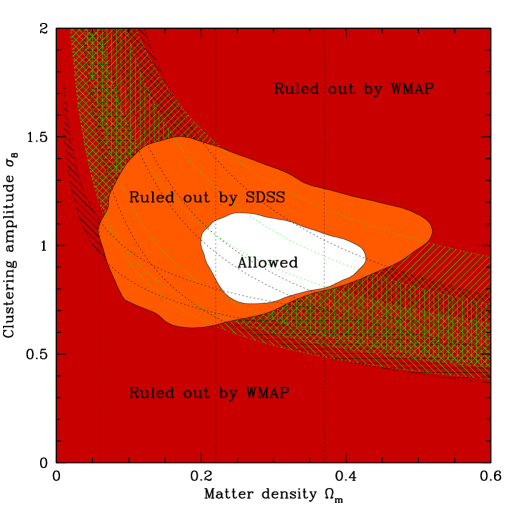
Figure 6: 95% constraints in the $(\Omega_{m},\sigma_{8})$ plane. Shaded dark red/grey region is ruled out by WMAP alone for 6-parameter “vanilla” models. The shaded light red/grey region is ruled out when adding SDSS information. The 95% confidence regions are hatched for various recent cluster (black) and lensing (green/grey) analyses as discussed in the text. The vertical lines indicate the constraints described in Bridle03 from mass-to-light ratios in galaxies and clusters ($0.06\mathrel{\hbox to0.0pt{\lower 3.0pt\hbox{$\mathchar 536\relax$}\hss}\raise 2.0pt\hbox{$\mathchar 316\relax$}}\Omega_{m}\mathrel{\hbox to0.0pt{\lower 3.0pt\hbox{$\mathchar 536\relax$}\hss}\raise 2.0pt\hbox{$\mathchar 316\relax$}}0.22$) and from cluster baryon fractions ($0.22\mathrel{\hbox to0.0pt{\lower 3.0pt\hbox{$\mathchar 536\relax$}\hss}\raise 2.0pt\hbox{$\mathchar 316\relax$}}\Omega_{m}\mathrel{\hbox to0.0pt{\lower 3.0pt\hbox{$\mathchar 536\relax$}\hss}\raise 2.0pt\hbox{$\mathchar 316\relax$}}0.37$).

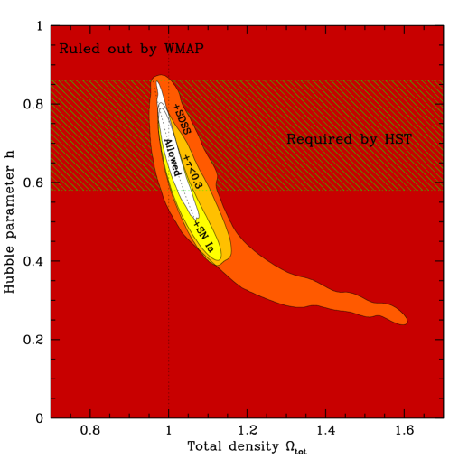
Figure 7: 95% constraints in the $(\Omega_{\rm tot},h)$ plane. Shaded dark red/grey region is ruled out by WMAP alone for 7-parameter curved models, showing that CMB fluctuations alone do not simultaneously show space to be flat and measure the Hubble parameter. The shaded light red/grey region is ruled out when adding SDSS information. Continuing inwards, the next two regions are ruled out when adding the $\tau<0.3$ assumption and when adding SN Ia information as well. The light hatched band is required by the HST key project Freedman01 . The dotted line shows the fit $h=0.7\Omega_{\rm tot}^{-5}$, explaining the origin of the accurate constraints $h\Omega_{\rm tot}^{5}=0.703^{+0.029}_{-0.024}$ and $\Omega_{\rm tot}(h/0.7)^{0.2}=1.001^{+0.008}_{-0.007}$ $(1\sigma)$.

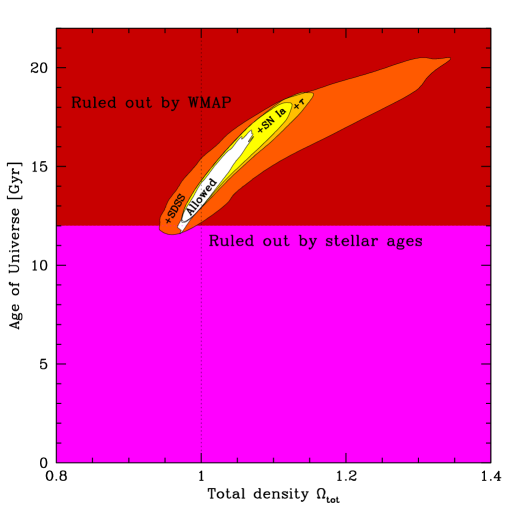
Figure 8: 95% constraints in the $(\Omega_{\rm tot},t_{0})$ plane. Shaded dark red/grey region is ruled out by WMAP alone for 7-parameter curved models, showing that CMB fluctuations do not simultaneously show space to be flat and measure the age of the Universe. The shaded light red/grey region is ruled out when adding SDSS information. Continuing inwards, the next two regions are ruled out when adding the $\tau<0.3$ assumption and when adding SN Ia information as well. Stellar age determinations (see text) rule out $t_{0}<12$ Gyr.

IV Curved models

Let us now spice up the vanilla model space by adding spatial curvature $\Omega_{k}$ as a free parameter, both to constrain the curvature and to quantify how other constraints get weakened when dropping the flatness assumption.

Figures 7 and 8 show that there is a strong degeneracy between the curvature of the universe $\Omega_{k}\equiv 1-\Omega_{\rm tot}$ and both the Hubble parameter $h$ and the age of the universe $t_{0}$, when constrained by WMAP alone (even with only the seven parameters we are now considering allowed to change); without further information or priors, one cannot simultaneously demonstrate spatial flatness and measure $h$ or $t_{0}$. We see that although WMAP alone abhors open models, requiring $\Omega_{\rm tot}\equiv\Omega_{m}+\Omega_{\Lambda}=1-\Omega_{k}\mathrel{\hbox to0.0pt{\lower 3.0pt\hbox{$\mathchar 536\relax$}\hss}\raise 2.0pt\hbox{$\mathchar 318\relax$}}0.9$ (95%), closed models with $\Omega_{\rm tot}$ as large as 1.4 are still marginally allowed provided that the Hubble parameter $h\sim 0.3$ and the age of the Universe $t_{0}\sim 20$ Gyr. Although most inflation models do predict space to be flat and closed inflation models require particularly ugly fine-tuning Linde0303245 , a number of recent papers on other subjects have considered nearly-flat models either to explain the low CMB quadrupole Efstathiou03 or for anthropic reasons Linde95 ; Vilenkin97 ; Q , so it is clearly interesting and worthwhile to test the flatness assumption observationally. In the same spirit, measuring the Hubble parameter $h$ independently of theoretical assumptions about curvature and measurements of galaxy distances at low redshift provides a powerful consistency check on our whole framework.

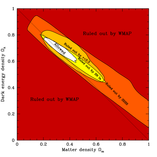
Figure 9: 95% constraints in the $(\Omega_{m},\Omega_{\Lambda})$ plane. Shaded dark red/grey region is ruled out by WMAP alone for 7-parameter curved models, illustrating the well-known geometric degeneracy between models that all have the same acoustic peak locations. The shaded light red/grey region is ruled out when adding SDSS information. Continuing inwards, the next two regions are ruled out when adding the $\tau<0.3$ assumption and when including SN Ia information as well. Models on the diagonal dotted line are flat, those below are open and those above are closed. The constraints in this plot agrees well with those in Figure 13 from Spergel03 when taking the $\tau$ prior into account.

Including SDSS information is seen to reduce the curvature uncertainty by about a factor of three. We also show the effect of adding the above-mentioned prior $\tau<0.3$ and SN Ia information from the 172 SN Ia compiled by Tonry03 , which is seen to further tighten the curvature constraints to $\Omega_{\rm tot}=1.01\pm 0.02$ ($1\sigma$), providing a striking vindication of the standard inflationary prediction $\Omega_{\rm tot}=1$. Yet even with all these constraints, a strong degeneracy is seen to persist between curvature and $h$, and curvature and $t_{0}$, so that the HST key project Freedman01 remains the most accurate measurement of $h$. If we add the additional assumption that space is exactly flat, then uncertainties shrink by factors around 3 and 4 for $h$ and $t_{0}$, respectively, still in beautiful agreement with other measurements. The age limit $t_{0}>12$ Gyr shown in Figure 8 is the 95% lower limit from white dwarf ages by Hansen02 ; for a thorough reviews of recent age determinations, see Spergel03 ; Lineweaver99 .

This curvature degeneracy is also seen in Figure 9, which illustrates that the existence of dark energy $\Omega_{\Lambda}>0$ is only required at high significance when augmenting WMAP with either galaxy clustering information or SN Ia information (as also pointed out by Spergel03 ). This stems from the well-known geometric degeneracy where $\Omega_{k}$ and $\Omega_{\Lambda}$ can be altered so as to leave the acoustic peak locations unchanged, which has been exhaustively discussed in the pre-WMAP literature — see, e.g., WhiteComplementarity ; parameters ; ZSS97 ; parameters2 ; EfstathiouBond99 .

In conclusion, we obtain sharp constraints on spatial curvature and interesting constraints on $h$, $t_{0}$ and $\Omega_{\Lambda}$, but only when combining WMAP with SDSS and/or other data. In other words, within the class of almost flat models, the WMAP-only constraints on $h$, $t_{0}$ and $\Omega_{\Lambda}$ are weak, and including SDSS gives a huge improvement in precision.

Since the constraints on $h$ and $t_{0}$ are further tightened by a large factor if space is exactly flat, can one justify the convenient assumption $\Omega_{\rm tot}=1$? Although WMAP alone marginally allows $\Omega_{\rm tot}=1.5$ (Figure 7), WMAP+SDSS shows that $\Omega_{\rm tot}$ is within 15% of unity. It may therefore be possible to bolster the case for perfect spatial flatness by demolishing competing theoretical explanations of the observed approximate flatness — for instance, it has been argued that if the near-flatness is due to an anthropic selection effect, then one expects departures from $\Omega_{\rm tot}\sim 1$ of order unity Linde95 ; Vilenkin97 , perhaps larger than we now observe. This approach is particularly promising if one uses a prior on $h$. Imposing a hard limit $0.58<h<0.86$ corresponding to the $2\sigma$ range from the HST key project Freedman01 , we obtain $\Omega_{\rm tot}=1.030^{+0.029}_{-0.029}$ from WMAP alone, $\Omega_{\rm tot}=1.023^{+0.020}_{-0.033}$ adding SDSS and $\Omega_{\rm tot}=1.010^{+0.018}_{-0.017}$ when also adding SN Ia and the $\tau<0.3$ prior.

V Testing inflation

V.1 The generic predictions

Two generic predictions from inflation are perfect flatness ($\Omega_{k}=0$, i.e., $\Omega_{\rm tot}\equiv 1-\Omega_{k}=1$) and approximate scale-invariance of the primordial power spectrum (${n_{s}}\sim 1$). Tables 2-4 show that despite ever-improving data, inflation still passes both of these tests with flying colors.

The tables show that although all cases we have explored are consistent with $\Omega_{\rm tot}={n_{s}}=1$, adding priors and non-CMB information shrinks the error bars by factors around 6 and 4 for $\Omega_{\rm tot}$ and ${n_{s}}$, respectively.

For the flatness test, Table 4 shows that $\Omega_{\rm tot}$ is within about 20% of unity with 68% confidence from WMAP alone without priors (even $\Omega_{\rm tot}\sim 1.5$ is allowed at the 95% confidence contour). When we include SDSS, the 68% uncertainty tightens to 10%, and the errors shrink impressively to the percent level with more data and priors: $\Omega_{\rm tot}=1.012^{+0.018}_{-0.022}$ using WMAP, SDSS, SN Ia and $\tau<0.3$.

For the scalar spectral index, Table 4 shows that ${n_{s}}\sim 1$ to within about 15% from WMAP alone without priors, tightening to ${n_{s}}=0.977^{+0.039}_{-0.025}$ when adding SDSS and assuming the vanilla scenario, so the cosmology community is rapidly approaching the milestone where the departures from scale-invariance that most popular inflation models predict become detectable.

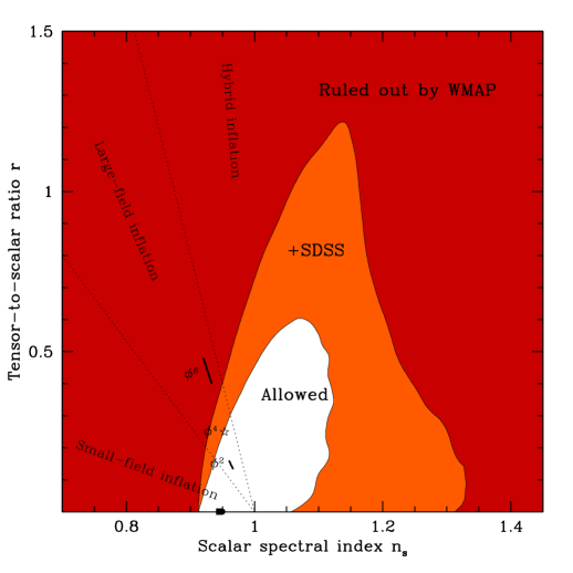
Figure 10: 95% constraints in the $({n_{s}},r)$ plane. Shaded dark red/grey region is ruled out by WMAP alone for 7-parameter models (the vanilla models plus $r$). The shaded light red/grey region is ruled out when adding SDSS information. The two dotted lines delimit the three classes of inflation models known as small-field, large-field and hybrid models. Some single-field inflation models make highly specific predictions in this plane as indicated. From top to bottom, the figure shows the predictions for $V(\phi)\propto\phi^{6}$ (line segment; ruled out by CMB alone), $V(\phi)\propto\phi^{4}$ (star; a textbook inflation model; on verge of exclusion) and $V(\phi)\propto\phi^{2}$ (line segment; the eternal stochastic inflation model; still allowed), and $V(\phi)\propto 1-(\phi/\phi_{*})^{2}$ (horizontal line segment with $r\sim 0$; still allowed). These predictions assume that the number of e-foldings between horizon exit of the observed fluctuations and the end of inflation is 64 for the $\phi^{4}$ model and between 50 and 60 for the others as per LiddleLeach03 .

V.2 Tensor fluctuation

The first really interesting confrontation between theory and observation was predicted to occur in the $({n_{s}},r)$ plane (Figure 10), and the first skirmishes have already begun. The standard classification of slow-roll inflation models DodelKinneyKolb97 ; LythRiotto99 ; LiddleLythBook characterized by a single field inflaton potential $V(\phi)$ conveniently partitions this plane into three parts (Figure 10) depending on the shape of $V(\phi)$:

1. Small-field models are of the form expected from spontaneous symmetry breaking, where the potential has negative curvature $V(\phi)^{\prime\prime}<0$ and the field $\phi$ rolls down from near the maximum, and all predict $r<{8\over 3}(1-{n_{s}})$, ${n_{s}}\leq 1$.

2. Large-field models are characteristic of so-called chaotic initial conditions, in which $\phi$ starts out far from the minimum of a potential with positive curvature ($V^{\prime\prime}(\phi)>0$), and all predict ${8\over 3}(1-{n_{s}})<r<8(1-{n_{s}})$, ${n_{s}}\leq 1$.

3. Hybrid models are characterized by a field rolling toward a minimum with $V\neq 0$. Although they generally involve more than one inflaton field, they can be treated during the inflationary epoch as single-field inflation with $V^{\prime\prime}>0$ and predict $r>{8\over 3}(1-{n_{s}})$, also allowing ${n_{s}}>1$.

These model classes are summarized in Table 6 together with a sample of special cases. For details and derivations of the tabulated constraints, see DodelKinneyKolb97 ; LythRiotto99 ; LiddleLythBook ; Peiris03 ; Kinney03 ; LiddleSmith03 ; Wands03 . For comparison with other papers, remember that we use the same normalization convention for $r$ as CMBfast and the WMAP team, where $r=-8{n_{t}}$ for slow-roll models. The limiting case between small-field and large-field models is the linear potential $V(\phi)\propto\phi$, and the limiting case between large-field and hybrid models is the exponential potential $V(\phi)\propto e^{\phi/\phi_{*}}$. The WMAP team Peiris03 further refine this classification by splitting the hybrid class into two: models with ${n_{s}}<1$ and models with ${n_{s}}>1$.

Table 6: Sample inflation model predictions. $N$ is the number of e-folds between horizon exit of the observed fluctuations and the end of inflation.

Model	Potential	$r$	${n_{s}}$
Small-field	$V^{\prime\prime}<0$	$r<{8\over 3}(1-{n_{s}})$	${n_{s}}\leq 1$
Parabolic	$V\propto 1-\left({\phi\over\phi_{*}}\right)^{2}$	$r=8(1-{n_{s}})e^{-N(1-{n_{s}})}\mathrel{\hbox to0.0pt{\lower 3.0pt\hbox{$\mathchar 536\relax$}\hss}\raise 2.0pt\hbox{$\mathchar 316\relax$}}0.06$	${n_{s}}<1$
Tombstone	$V\propto 1-\left({\phi\over\phi_{*}}\right)^{4}$	$r\mathrel{\hbox to0.0pt{\lower 3.0pt\hbox{$\mathchar 536\relax$}\hss}\raise 2.0pt\hbox{$\mathchar 316\relax$}}10^{-3}$	${n_{s}}=1-{3\over N}\sim 0.95$
	$V\propto 1-\left({\phi\over\phi_{*}}\right)^{p}$, $p>2$	$r\mathrel{\hbox to0.0pt{\lower 3.0pt\hbox{$\mathchar 536\relax$}\hss}\raise 2.0pt\hbox{$\mathchar 316\relax$}}10^{-3}$	${n_{s}}=1-{2\over N}{p-1\over p-2}\mathrel{\hbox to0.0pt{\lower 3.0pt\hbox{$\mathchar 536\relax$}\hss}\raise 2.0pt\hbox{$\mathchar 318\relax$}}0.93$
Linear	$V\propto\phi$	$r={8\over 3}(1-{n_{s}})$	${n_{s}}\leq 1$
Large-field	$V^{\prime\prime}>0$	${8\over 3}(1-{n_{s}})<r<8(1-{n_{s}})$	${n_{s}}\leq 1$
Power-law	$V\propto\phi^{p}$	$r={4p\over N}$	${n_{s}}=1-{{1+p/2}\over N}$
Quadratic	$V\propto\phi^{2}$	$r={8\over N}\sim 0.15$	${n_{s}}=1-{2\over N}\sim 0.96$
Quartic	$V\propto\phi^{4}$	$r={16\over N}\sim 0.29$	${n_{s}}=1-{3\over N}\sim 0.95$
Sextic	$V\propto\phi^{6}$	$r={24\over N}\sim 0.44$	${n_{s}}=1-{4\over N}\sim 0.93$
Exponential	$V\propto e^{\phi/\phi_{*}}$	$r=8(1-{n_{s}})$	${n_{s}}\leq 1$
Hybrid	$V^{\prime\prime}>0$	$r>{8\over 3}(1-{n_{s}})$	Free

Many inflationary theorists had hoped that early data would help distinguish between these classes of models, but Figure 10 shows that all three classes are still allowed.

What about constraints on specific inflation models as opposed to entire classes? Here the situation is more interesting. Some models, such as hybrid ones, allow two-dimensional regions in this plane. Table 6 shows that many other models predict a one-dimensional line or curve in this plane. Finally, a handful of models are extremely testable, making firm predictions for both ${n_{s}}$ and $r$ in terms of $N$, the number of e-foldings between horizon exit of the observed fluctuations and the end of inflation. Recent work HuiDodel03 ; LiddleLeach03 has shown that $50\mathrel{\hbox to0.0pt{\lower 3.0pt\hbox{$\mathchar 536\relax$}\hss}\raise 2.0pt\hbox{$\mathchar 316\relax$}}N\mathrel{\hbox to0.0pt{\lower 3.0pt\hbox{$\mathchar 536\relax$}\hss}\raise 2.0pt\hbox{$\mathchar 316\relax$}}60$ is required for typical inflation models. The quartic model $V\sim\phi^{4}$ is an anomaly, requiring $N\approx 64$ with very small uncertainty. Figure 10 shows that power law models $V\propto\phi^{p}$ are ruled out by CMB alone for $p=6$ and above. Figure 10 indicates that the textbook $V\propto\phi^{4}$ model (indicated by a star in the figure) is marginally allowed. Peiris03 found it marginally ruled out, but this assumed $N=50$ — the subsequent result $N\approx 64$ LiddleLeach03 pushes the model down to the right and make it less disfavored. $V\propto\phi^{2}$ has been argued to be the most natural power-law model, since the Taylor expansion of a generic function near its minimum has this shape and since there is no need to explain why quantum corrections have not generated a quadratic term. This potential is used in the stochastic eternal inflation model LindeBook , and is seen to be firmly in the allowed region, as are the small-field “tombstone model” from Table 6 and the GUT-scale model of KyaeShafi0302504 (predicting ${n_{s}}=1-1/N\approx 0.98$, $r\approx 10^{-8}$).

In conclusion, Figure 10 shows that observations are now beginning to place interesting constraints on inflation models in the $({n_{s}},r)$-plane. As these constraints tighten in coming years, they will allow us to distinguish between many of the prime contenders. For instance, the stochastic eternal inflation model predicting $({n_{s}},r)\approx(0.96,0.15)$ will become distinguishable from models with negligible tensors, and in the latter category, small-field models with, say, ${n_{s}}\mathrel{\hbox to0.0pt{\lower 3.0pt\hbox{$\mathchar 536\relax$}\hss}\raise 2.0pt\hbox{$\mathchar 316\relax$}}0.95$, will become distinguishable from the scale-invariant case ${n_{s}}=1$.

V.3 A running spectral index?

Typical slow-roll models predict not only negligible spatial curvature, but also that the running of the spectral index $\alpha$ is unobservably small. We therefore assumed $\Omega_{k}=\alpha=0$ when testing such models above.

Let us now turn to the issue of searching for departures from a power law primordial power spectrum. This issue has generated recent interest after the WMAP team claim that $\alpha<0$ was favored over $\alpha=0$, at least at modest statistical significance, with the preferred value being $\alpha\sim-0.07$ Peiris03 ; Spergel03 .

Slow-roll models typically predict $|\alpha|$ of order $N^{-2}$; for these models, $|\alpha|$ is rarely above $10^{-3}$, much smaller than the WMAP-team preferred value. Those inflation models that do predict such a strong second derivative of the primordial power spectrum (in log-log space) tend to produce substantial third and higher derivatives as well, so that a parabolic curve parametrized by $A_{s}$, ${n_{s}}$ and $\alpha$ is a poor approximation of the model (e.g., Lidsey03 ). Lacking strong theoretical guidance one way or another, we therefore drop our priors on $\Omega_{k}$ and $r$ when constraining $\alpha$.

Tables 2 and 3 show that our best-fit $\alpha$-values agree with those of Peiris03 , but are consistent with $\alpha=0$, since the 95% error bars are of order $0.1$. They show that $\chi^{2}$ drops by only 5 relative to vanilla models, which is not statistically significant because a drop of 3 is expected from freeing the three parameters $\Omega_{k}$, $r$ and $\alpha$. Moreover, we see that our WMAP-only constraint is similar to our WMAP+SDSS constraint, showing that any hint of running comes from the CMB alone, most likely from the low quadrupole power Spergel03 ; see also Efstathiou03b ; smalluniverse . This is at least qualitatively consistent with the WMAP team analysis Spergel03 ; apart from the low quadrupole, most of the evidence that $\alpha\neq 0$ comes from CMB fluctuation data on small scales (e.g., the CBI data CBI02 ) and measurements of the small-scale fluctuations from the Ly$\alpha$ forest; indeed, including the 2dFGRS data slightly weakens the case for running. For the Ly$\alpha$ forest case, the key issue is the extent to which the measurement uncertainties have been adequately modeled Seljak03 , and this should be clarified by the forthcoming Ly$\alpha$ forest measurements from the SDSS.

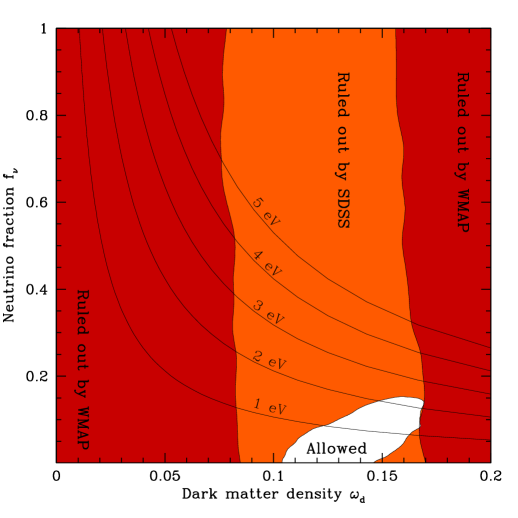
Figure 11: 95% constraints in the $(\omega_{d},f_{\nu})$ plane. Shaded dark red/grey region is ruled out by WMAP alone when neutrino mass is added to the 6 “vanilla” models. The shaded light red/grey region is ruled out when adding SDSS information. The five curves correspond to $M_{\nu}$, the sum of the neutrino masses, equaling 1, 2, 3, 4 and 5 eV, respectively — barring sterile neutrinos, no neutrino can have a mass exceeding $\sim M_{\nu}/3.$

VI Neutrino mass

It has long been known neutrinos that galaxy surveys are sensitive probes of neutrino mass, since they can detect the suppression of small-scale power caused by neutrinos streaming out of dark matter overdensities. For detailed discussion of post-WMAP astrophysical neutrino constraints, see Spergel03 ; Hannestad0303076 ; ElgaroyLahav0303089 ; BashinskySeljak03 ; Hannestad0310133 , and for an up-to-date review of the theoretical and experimental situation, see King03 .

Our neutrino mass constraints are shown in the $M_{\nu}$-panel of Figure 2, where we allow our standard 6 “vanilla” parameters and $f_{\nu}$ to be free. The most favored value is $M_{\nu}=0$, and obtain a 95% upper limit $M_{\nu}<1.7\>$eV. Figure 11 shows that WMAP alone tells us nothing whatsoever about neutrino masses and is consistent with neutrinos making up 100% of the dark matter. Rather, the power of WMAP is that it constrains other parameters so strongly that it enables large-scale structure data to measure the small-scale $P(k)$-suppression that massive neutrinos cause.

The sum of the three neutrino masses (assuming standard freezeout) is KolbTurnerBook $M_{\nu}\approx(94.4\>{\rm eV})\omega_{d}f_{\nu}.$ The neutrino energy density must be very close to the standard freezeout density synch1 ; synch2 ; synch3 , given the large mixing angle solution to the solar neutrino problem and near maximal mixing from atmospheric results— see Kearns02 ; Bahcall03 for up-to-date reviews. Any substantial asymmetries in neutrino density from the standard value would be “equilibrated” and produce a primordial ⁴He abundance inconsistent with that observed.

Our upper limit is complemented by the lower limit from neutrino oscillation experiments. Atmospheric neutrino oscillations show that there is at least one neutrino (presumably mostly a linear combination of $\nu_{\mu}$ and $\nu_{\tau}$) whose mass exceeds a lower limit around $0.05\>$eV Kearns02 ; King03 . Thus the atmospheric neutrino data corresponds to a lower limit $\omega_{\nu}\mathrel{\hbox to0.0pt{\lower 3.0pt\hbox{$\mathchar 536\relax$}\hss}\raise 2.0pt\hbox{$\mathchar 318\relax$}}0.0005$, or $f_{\nu}\mathrel{\hbox to0.0pt{\lower 3.0pt\hbox{$\mathchar 536\relax$}\hss}\raise 2.0pt\hbox{$\mathchar 318\relax$}}0.004$. The solar neutrino oscillations occur at a still smaller mass scale, perhaps around $0.008\>$eV sno0309004 ; King03 ; Bahcall03 . These mass-splittings are much smaller than 1.7 eV, suggesting that all three mass eigenstates would need to be almost degenerate for neutrinos to weigh in near our upper limit. Since sterile neutrinos are disfavored from being thermalized in the early universe fournu1 ; fournu2 , it can be assumed that only three neutrino flavors are present in the neutrino background; this means that none of the three neutrinos can weigh more than about $1.7/3=0.6$ eV. The mass of the heaviest neutrino is thus in the range $0.04-0.6$ eV.

A caveat about non-standard neutrinos is in order. To first order, our cosmological constraint probes only the mass density of neutrinos, $\rho_{\nu}$, which determines the small-scale power suppression factor, and the velocity dispersion, which determines the scale below which the suppression occurs. For the low mass range we have discussed, the neutrino velocities are high and the suppression occurs on all scales where SDSS is highly sensitive. We thus measure only the neutrino mass density, and our conversion of this into a limit on the mass sum assumes that the neutrino number density is known and given by the standard model freezeout calculation, 112 cm^-3. In more general scenarios with sterile or otherwise non-standard neutrinos where the freezeout abundance is different, the conclusion to take away is an upper limit on the total light neutrino mass density of $\rho_{\nu}<4.8\times 10^{-28}$kg/m³ (95%). To test arbitrary nonstandard models, a future challenge will be to independently measure both the mass density and the velocity dispersion, and check whether they are both consistent with the same value of $M_{\nu}$.

The WMAP team obtains the constraint $M_{\nu}<0.7$ eV Spergel03 by combining WMAP with the 2dFGRS. This limit is a factor of three lower than ours because of their stronger priors, most importantly that on galaxy bias $b$ determined using a bispectrum analysis of the 2dF galaxy clustering dataVerde02 . This bias was measured on scales $k\sim 0.2-0.4h$/Mpc and assumed to be the same on the scales $k<0.2h$/Mpc that were used in the analysis. In this paper, we prefer not to include such a prior. Since the bias is marginalized over, our SDSS neutrino constraints come not from the amplitude of the power spectrum, only from its shape. This of course allows us to constrain $b$ from WMAP+SDSS directly; we find values consistent with unity (for $L^{*}$ galaxies) in almost all cases (Tables 3 and 4). A powerful consistency test is that our corresponding value $\beta=0.54^{+0.06}_{-0.05}$ from WMAP+SDSS agrees well with the value $\beta\sim 0.5$ measured from redshift space distortions in sdsspower .

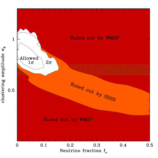
Figure 12: Constraints in the $(f_{\nu},\sigma_{8})$ plane. Shaded dark red/grey region is ruled out by WMAP alone ($95\%$) when neutrino mass is added to the 6 “vanilla” models. The shaded light red/grey region is ruled out when adding SDSS information. The recent claim that $f_{\nu}>0$ Allen0306386 hinges on assuming that galaxy clusters require low $\sigma_{8}$-values (shaded horizontal band) and dissolves when using what we argue are more reasonable uncertainties in the cluster constraints.

Seemingly minor assumptions can make a crucial difference for neutrino conclusions, as discussed in detail in Spergel03 ; Hannestad0303076 ; ElgaroyLahav0303089 . A case in point is a recent claim that nonzero neutrino mass has been detected by combining WMAP, 2dFGRS and galaxy cluster data Allen0306386 . Figure 2 in that paper (middle left panel) shows that nonzero neutrino mass is strongly disfavored only when including data on X-ray cluster abundance, which is seen (lower middle panel) to prefer a low normalization of order $\sigma_{8}\approx 0.70\pm 0.05$ (68%). Figure 12 provides intuition for the physical origin on the claimed neutrino mass detection. Since WMAP fixes the normalization at early times before neutrinos have had their suppressing effect, we see that the WMAP-allowed $\sigma_{8}$-value drops as the neutrino fraction $f_{\nu}$ increases. A very low $\sigma_{8}$-value therefore requires a nonzero neutrino fraction. The particular cluster analysis used by Allen0306386 happens to give one of the lowest $\sigma_{8}$-values in the recent literature. Table 5 and Figure 6 show a range of $\sigma_{8}$ values larger than the individual quoted errors, implying the existence of significant systematic effects. If we expand the error bars on the cluster constraints to $\sigma_{8}=0.8\pm 0.2$, to reflect the spread in the recent literature, we find that the evidence for a cosmological neutrino mass detection goes away. The sensitivity of neutrino conclusions to cluster $\sigma 8$ normalization uncertainties was also discussed in Allen0306386 .

VII Dark energy equation of state

Although we now know its present density fairly accurately, we know precious little else about the dark energy, and post-WMAP research is focusing on understanding its nature Melchiorri0211522 ; Barreiro03 ; dedeo03 ; CaldwellDoran03 ; CaldwellKamionWeinberg03 ; Caldwell03 ; Balakin03 ; Weller03 ; Kunz03 . Above we have assumed that the dark energy behaves as a cosmological constant with its density independent of time, i.e., that its equation of state $w=-1$. Figure 2 and Figure 13 show our constraints on $w$, assuming that the dark energy is homogeneous, i.e., does not cluster. Although our analysis adds improved galaxy and SN Ia data to that of the WMAP team Spergel03 and uses different assumptions, Figure 13 agrees well with Figure 11 from Spergel03 and our conclusions are qualitatively the same: adding $w$ as a free parameter does not help improve $\chi^{2}$ for the best fit, and all data are consistent with the vanilla case $w=-1$, with uncertainties in $w$ at the 20% level. Melchiorri0211522 ; Weller03 obtained similar constraints with different data and an $h$-prior.

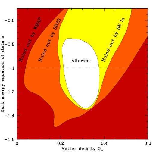
Figure 13: 95% constraints in the $(\Omega_{m},w)$ plane. Shaded dark red/grey region is ruled out by WMAP alone when equation of state $w$ is added to the 6 “vanilla” parameters. The shaded light red/grey region is ruled out when adding SDSS information, and the yellow/very light grey region is excluded when including SN Ia information as well.

Tables 2 and 3 show the effect of dropping the $w=-1$ assumption on other parameter constraints. These effects are seen to be similar to those of dropping the flatness assumption, but weaker, which is easy to understand physically. As long as there are no spatial fluctuations in the dark energy (as we have assumed), changing $w$ has only two effects on the CMB: it shifts the acoustic peaks sideways by altering the angle-distance relation, and it modifies the late Integrated Sachs-Wolfe (ISW) effect. Its only effect effect on the matter power spectrum is to change its amplitude via the linear growth factor. The exact same things can be said about the parameters $\Omega_{\Lambda}$ and $\Omega_{k}$, so the angle-diameter degeneracy becomes a two-dimensional surface in the three-dimensional space ($\Omega_{k},\Omega_{\Lambda},w$), broken only by the late ISW effect. Since the peak-shifting is weaker for $w$ than for $\Omega_{k}$ (for changes generating comparable late ISW modification), adding $w$ to vanilla models wreaks less havoc with, say, $h$ than does adding $\Omega_{k}$ to vanilla models (Section IV).

VIII Discussion and conclusions

We have measured cosmological parameters using the three-dimensional power spectrum $P(k)$ from over 200,000 galaxies in the Sloan Digital Sky Survey (SDSS) in combination with WMAP and other data. Let us first discuss what we have and have not learned about cosmological parameters, then summarize what we have and have not learned about the underlying physics.

VIII.1 The best fit model

All data we have considered are consistent with a “vanilla” flat adiabatic $\Lambda$CDM model with no tilt, running tilt, tensor fluctuations, spatial curvature or massive neutrinos. Readers wishing to choose a concordance model for a calculational purposes using Ockham’s razor can adopt the best fit “vanilla lite” model

$$(\tau,\Omega_{\Lambda},\omega_{d},\omega_{b},A_{s})=(0.17,0.72,0.12,0.024,0.89)$$ (2)

(Table 4, second last column). Note that this is even simpler than 6-parameter vanilla models, since it has ${n_{s}}=1$ and only 5 free parameters Easther03 . A more theoretically motivated 5-parameter model is that of the arguably most testable inflation model, $V\propto\phi^{2}$ stochastic eternal inflation, which predicts $({n_{s}},r)=(0.15,0.96)$ (Figure 10) and prefers

$$(\tau,\Omega_{\Lambda},\omega_{d},\omega_{b},A_{s})=(0.09,0.68,0.123,0.023,0.75)$$ (3)

(Table 4, second last column).

Note that these numbers are in substantial agreement with the results of the WMAP team Spergel03 , despite a completely independent analysis and independent redshift survey data; this is a powerful confirmation of their results and the emerging standard model of cosmology. Equally impressive is the fact that we get similar results and error bars when replacing WMAP by the combined pre-WMAP CMB data (compare the last columns of Table 3). In other words, the concordance model and the tight constraints on its parameters are no longer dependent on any one data set — everything still stands even if we discard either WMAP or pre-WMAP CMB data and either SDSS or 2dFGRS galaxy data. No single data set is indispensable.

As emphasized by the WMAP team, it is remarkable that such a broad range of data are describable by such a small number of parameters. Indeed, as is apparent from Tables 2–4, $\chi^{2}$ does not improve significantly upon the addition of further parameters for any set of data. However, the “vanilla lite” model is not a complete and self-consistent description of modern cosmology; for example, it ignores the well-motivated inflationary arguments for expecting ${n_{s}}\neq 1$.

VIII.2 Robustness to physical assumptions

On the other hand, the same criticism can be leveled against 6-parameter vanilla models, since they assume $r=0$ even though some of the most popular inflation models predict a significant tensor mode contribution. Fortunately, Table 3 shows that augmenting vanilla models with tensor modes has little effect on other parameters and their uncertainties, mainly just raising the best fit spectral index ${n_{s}}$ from 0.98 to 1.01.

Another common assumption is that the neutrino density $f_{\nu}$ is negligible, yet we know experimentally that $f_{\nu}>0$ and there is an anthropic argument for why neutrinos should make a small but non-negligible contribution anthroneutrino . The addition of neutrinos changes the slope of the power spectrum on small scales; in particular, when we allow $f_{\nu}$ to be a free parameter, the value of $\sigma_{8}$ drops by 10% and $\Omega_{m}$ increases by 25% (Table 2).

We found that the assumption with the most striking implications is that of perfect spatial flatness, $\Omega_{\rm tot}=1$ — dropping it dramatically weakens the limits on the Hubble parameter and the age of the Universe, allowing $h=0.5$ and $t_{0}=18$ Gyr. Fortunately, this flatness assumption is well-motivated by inflation theory; while anthropic explanations exist for the near flatness, they do not predict the Universe to be quite as flat as it is now observed to be.

Constraints on other parameters are also somewhat weakened by allowing a running spectral index $\alpha\neq 0$ and an equation of state $w\neq-1$, but we have argued that these results are more difficult to take seriously theoretically. It is certainly worthwhile testing whether ${n_{s}}$ depends on $k$ and whether $\Omega_{\Lambda}$ depends on $z$, but parametrizing such departures in terms of constants $\alpha$ and $w$ to quantify the degeneracy with other parameters is unconvincing, since most inflation models predict observably large $|\alpha|$ to depend strongly on $k$ and observably large $|w+1|$ can depend strongly on $z$.

It is important to parametrize and constrain possible departures the current cosmological framework: any test that could have falsified it, but did not, bolsters its credibility. Post-WMAP work in this spirit has included constraints on the dark energy sound speed Weller03 and time dependence WangMukherjee0312192 ; Alam0311364 , the fine structure constant Rocha03 , the primordial helium abundance Trotta03 ; Huey03 , isocurvature modes Crotty03 and features in the primordial power spectrum Bridle0302306 ; Hannestad0311491 .

VIII.3 Robustness to data details

How robust are our cosmological parameter measurements to the choice of data and to our modeling thereof?

For the CMB, most of the statistical power comes from the unpolarized WMAP data, which we confirmed by repeating our 6-parameter analysis without polarization information. The main effect of adding the polarized WMAP data is to give a positive detection of $\tau$ (Section VIII.4.4 below). The quantity $\sigma_{8}e^{-\tau}$ determines the amplitudes of acoustic peak amplitudes, so the positive detection of $\tau$ leads to a value of $\sigma_{8}$ 15% higher than without the polarization data included.

For the galaxy $P(k)$ data, there are options both for what data set to use and how to model it. To get a feeling for the quantitative importance of choices, we repeat a simple benchmark analysis for a variety of cases. Let us measure the matter density $\Omega_{m}$ using galaxy data alone, treating $A_{s}$ as a second free parameter and fixing all others at the values $\Omega_{k}=f_{\nu}=\alpha=0$, $\omega_{b}=0.024$, ${n_{s}}=1$, $w=-1$, $b=1$ and $h=0.72$. Roughly speaking, we are thus fitting the measured galaxy power spectrum to a power spectrum curve that we can shift horizontally (with our “shape parameter” $\Omega_{m}$) and vertically (with $A_{s}$). We have chosen this particular example because, as described in Section III, it is primarily this shape parameter measurement that breaks the WMAP banana degeneracy. The parameters $\tau$ and $r$ of course have no effect on $P(k)$, and the remaining two are determined by the matter density via the identities $\Omega_{\Lambda}=1-\Omega_{m}$, $\omega_{d}=h^{2}\Omega_{m}-\omega_{b}$.

Table 7: Robustness to data and method details.

Analysis	$\Omega_{m}$
Baseline	$0.291^{+0.033}_{-0.027}$
$k_{\rm max}=0.15h/$Mpc	$0.297^{+0.038}_{-0.032}$
$k_{\rm max}=0.1h/$Mpc	$0.331^{+0.079}_{-0.051}$
No bias correction	$0.256^{+0.027}_{-0.024}$
Linear $P(k)$	$0.334^{+0.027}_{-0.024}$
2dFGRS	$0.251^{+0.036}_{-0.027}$

Our results are summarized in Table 7. We stress that they should not be interpreted as realistic measurements of $\Omega_{m}$, since the other parameters have not been marginalized over. This is why the error bars are seen to be smaller even than when WMAP was included above (last column of Table 4).

To avoid uncertainties associated with nonlinear redshift space distortions and scale-dependent galaxy bias, we have used SDSS measurements of $P(k)$ only for $k\leq k_{\rm max}$ throughout this paper, chosing $k_{\rm max}=0.2h/$Mpc as recommended in sdsspower . The WMAP team made this same choice $k_{\rm max}=0.2h/$Mpc when analyzing the 2dFGRS data Verde03 . An option would be to tighten this cut to be still more cautious. Table 7 shows that cutting back to $k_{\rm max}=0.15h/$Mpc has essentially no effect on the best-fit $\Omega_{m}$-value and increases error bars by about 20%. Cutting back all the way down to $k_{\rm max}=0.1h/$Mpc is seen to more than double the baseline error bars, the baseline measurement lying about $0.6\sigma$ below the new best fit.

As described in sdsspower , the SDSS measurements were corrected for luminosity-dependent bias. Table 7 shows that if this were not done, $\Omega_{m}$ would drop by about 0.03, or $1\sigma$. This correction is of course not optional. However, if the correction itself were somehow inaccurate at say the 10% level, one would expect a bias in $\Omega_{m}$ around 0.003.

Just like the WMAP team Spergel03 ; Verde03 , we have used the nonlinear matter power spectrum for all our analysis. Table 7 shows that if we had used the linear spectrum instead, then $\Omega_{m}$ would rise by about 0.04, or $1.3\sigma$. This happens because the linear power spectrum is redder, with less small-scale power, which can be roughly offset by raising $\Omega_{m}$ and hence shifting the curve to the right. Like the above-mentioned correction for luminosity-dependent bias, correction for nonlinearities must be included. However, given the large uncertainties about how biasing behaves in this quasilinear regime, it may well be that this correction is only accurate to 25%, say, in which case we would expect an additional uncertainty in $\Omega_{m}$ at the 0.01 level.

Finally, we have repeated the analysis using an entirely different dataset, the $P(k)$-measurement from the 2dFGRS team Percival01 . Although the WMAP team used $k_{\rm max}=0.2h/$Mpc, we used the data available online with $k_{\rm max}=0.15h/$Mpc here as recommended by the 2dFGRS team Percival01 . Table 7 shows that 2dFGRS measures a slightly redder power spectrum than SDSS, corresponding to $\Omega_{m}$ down by 0.04, or $1.3\sigma$.

In conclusion, we see that a number of issues related to data selection and modeling can have noticeable effects on the results. Internally to SDSS, such effects could easily change $\Omega_{m}$ by as much as 0.01, and the 2dFGRS difference is about 0.04, or one standard deviation — roughly what one would expect with two completely independent data sets.

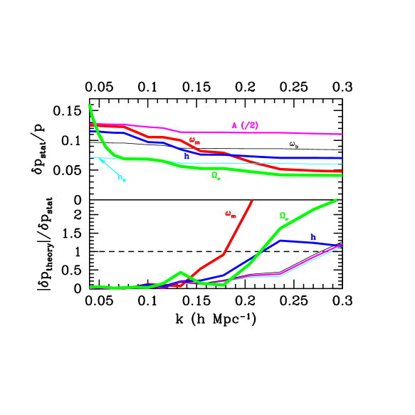
Figure 14: Effect of increasing the amount of SDSS data used, given by the maximum $k$-value used. Top panel shows how the relative errors on various parameters shrink as more data is included. For the neutrino density $\Omega_{\nu}\equiv f_{\nu}\Omega_{d}$, the absolute rather than relative error is shown. Bottom panel shows the ratio of systematic errors to statistical errors (from top panel) grows as smaller scales are included. This is for the extreme case where nonlinear corrections are present but completely ignored, which we view as a worst-case scenario.

To quantify the effect of systematic uncertainties when both other parameters and WMAP data are included, we carry out a second testing exercise. Using the Fisher-matrix technique of KnoxScocciDodel98 , we compute how our best-fit parameter values shift in response to a systematic bias in the theoretically computed power spectrum $P(k)$. To be conservative, we make the rather extreme assumption that the measurements correspond to the nonlinear power spectrum but that the analysis ignores nonlinear corrections entirely, simply fitting to the linear power spectrum. Although we view this as a worst-case scenario, it provides an instructive illustration of how problems related to nonlinear redshift space distortions and scale-dependent biasing might scale with $k_{\rm max}$, the largest $k$-band included.

Our results are shown in Figure 14. The upper panel shows how the constraints from WMAP alone (on left side of figure) gradually improve as more SDSS data are included. The dramatic neutrino improvement seen at small $k_{\rm max}$ is due to WMAP alone leaving the neutrino fraction unconstrained. The other parameters where SDSS helps the most are seen to be $\omega_{\rm m}$ and $h$, which can be understood based on our discussion in Section III. The SDSS power spectrum we have used does not probe to scales much smaller than $k\sim 0.2$, which is why little further improvement is seen beyond this value.

The lower panel shows the ratio of the above-mentioned systematic error to the statistical error for each parameter. We see that the most sensitive parameter is $\omega_{\rm m}$, which justifies our singling it out for special scrutiny above in Table 7 (where $\omega_{\rm m}$ is equivalent to $\Omega_{m}$ since we kept $h$ fixed). Although ${n_{s}}$ also partially mimics the nonlinear correction and perhaps scale-dependent bias, it is seen to be somewhat less sensitive. Our Fisher matrix estimate is seen to be somewhat overly pessimistic for $\Omega_{m}$, predicting that neglecting nonlinearities shifts $\omega_{\rm m}$ by of order $2\sigma$ for $k_{\rm max}=0.2h/$Mpc whereas the brute force analysis in Table 7 shows the shift to be only about half as large even when WMAP is ignored. The sensitivity to $h$ is linked to the $\Omega_{m}$-sensitivity by the banana in Figure 5. The $\Omega_{\nu}$-sensitivity comes from the small-scale neutrino $P(k)$-suppression being similar to the suppression in going from nonlinear to linear $P(k)$-modeling.

In conclusion, as long as errors in the modeling of nonlinear redshift distortions and bias are not larger than the nonlinear correction itself, we expect our uncertainties with $k_{\rm max}=0.2h/$Mpc to be dominated by statistical rather than systematic errors. The fact that cutting back to $k_{\rm max}=0.15h/$Mpc left our results virtually unchanged (Table 7) supports this optimistic conclusion. Indeed, Figure 14 shows that with $k_{\rm max}=0.15h/$Mpc, the reader wanting to perform a simple analysis can even use the linear $P(k)$ to good approximation.

However, both statistical errors and the systematic errors we have discussed in this section are dwarfed by the effects of changing theoretical priors. For instance, Table 2 shows that $\Omega_{m}$ increases by 0.08 when dropping either the assumption of negligible neutrinos or the assumption of negligible curvature. Moreover, to place this in perspective, all Bayesian analysis using Monte Carlo Markov Chains implicitly assumes a uniform prior on the space of the parameters where the algorithm jumps around, and different authors make different choices for these parameters, which can make a substantial difference.

A final source of potential uncertainties involves bugs and algorithmic errors in the analysis software. To guard against this, we performed two completely independent analyses for many of the parameter spaces that we have tabulated, one using the Monte Carlo Markov Chain method described in Appendix A (coded up from scratch) and the second using the publicly available CosmoMC package Lewis02 with appropriate modifications. We found excellent agreement between the two sets of results, with all differences much smaller than the statistical errors and prior-related uncertainties.

VIII.4 What have we learned about physics?

The fact that any simple model fits such accurate and diverse measurements is impressive evidence that the basic theoretical framework of modern cosmology is correct, and that we need to take its implications seriously however surprising they may be. What are these implications?

VIII.4.1 Inflation

The two generic predictions of perfect flatness ($|\Omega_{k}|\mathrel{\hbox to0.0pt{\lower 3.0pt\hbox{$\mathchar 536\relax$}\hss}\raise 2.0pt\hbox{$\mathchar 316\relax$}}10^{-5}$) and near scale-invariance have passed yet another test with flying colors. We find no evidence for running tilt. We also find no evidence for gravitational waves, and are therefore unable to measure the tensor spectral index and test the inflationary consistency relation $r=-8{n_{t}}$. The most interesting confrontation between theory and observation is now occurring in the $({n_{s}},r)$ plane (Figure 10). We confirm the conclusion Peiris03 that most popular models are still allowed, notably even stochastic eternal inflation with its prediction $({n_{s}},r)\approx(0.96,0.16)$, but modest data improvements over the next few years could decimate the list of viable inflationary candidates and rival models Song03 .

VIII.4.2 Dark energy

Since its existence is now supported by three independent lines of evidence (SN Ia, power spectrum analysis such as ours, the late ISW effect Boughn03 ; Nolta03 ; Fosalba0305468 ; Fosalba03 ; Scranton03 ; Afshordi03 ) and its current density is well known (the last column off Table 2 gives $\Omega_{\Lambda}=0.70\pm 0.04$), the next challenge is clearly to measure whether its density changes with time. Although our analysis adds improved galaxy and SN Ia data to that of the WMAP team Spergel03 , our conclusions are qualitatively the same: all data are consistent with the density being time-independent as for a simple cosmological constant ($w=-1$), with uncertainties in $w$ at the 20% level.

VIII.4.3 Cold and hot dark matter

We measure the density parameter for dark matter to be $\omega_{d}=0.12\pm 0.01$ fairly robustly to theoretical assumptions, which corresponds to a physical density of $2.3\times 10^{-27}$kg/m³ $\pm 10\%$. Given the WMAP information, SDSS shows that no more than about 12% of this dark matter can be due to massive neutrinos, giving a 95% upper limit to the sum of the neutrino masses $M_{\nu}<1.7$ eV. Barring sterile neutrinos, this means that no neutrino mass can exceed $M_{\nu}/3=0.6$ eV. Spergel03 quotes a tighter limit by assuming a strong prior on galaxy bias $b$. We show that the recent claim of a neutrino mass detection $M_{\nu}\mathrel{\hbox to0.0pt{\lower 3.0pt\hbox{$\mathchar 536\relax$}\hss}\raise 2.0pt\hbox{$\mathchar 318\relax$}}0.6$ eV by Allen et al. hinges crucially on a particular low galaxy cluster $\sigma_{8}$ measurement and goes away completely when expanding the cluster $\sigma_{8}$ uncertainty to reflect the spread in the literature.

VIII.4.4 Reionization and astronomy parameters

We confirm the WMAP team Spergel03 measurement of early reionization, $\tau=0.12^{+0.08}_{-0.06}$. This hinges crucially on the WMAP polarization data; using only the unpolarized WMAP power spectrum, our analysis prefers $\tau=0$ and gives an upper limit $\tau<0.23$ (95%).

Assuming the vanilla model, our Hubble parameter measurement $h\approx 0.70^{+0.04}_{-0.03}$ agrees well with the HST key project measurement $h=0.72\pm 0.07$ Freedman01 . It is marginally lower than the WMAP team value $h\approx 0.73\pm 0.03$ because the SDSS power spectrum has a slightly bluer slope than that of the 2dFGRS, favoring slightly higher $\Omega_{m}$-values (we obtain $\Omega_{m}=0.30\pm 0.04$; the WMAP team quote $\Omega_{m}=0.26\pm 0.05$ Spergel03 ).

VIII.5 What have we not learned?

The cosmology community has now established the existence of dark matter, dark energy and near-scale invariant seed fluctuations. Yet we do not know why they exist or the physics responsible for generating them. Indeed, it is striking that standard model physics fails to explain any of the four ingredients of the cosmic matter budget: it gives too small CP-violation to explain baryogenesis, does not produce dark matter particles, does not produce dark energy at the observed level and fails to explain the small yet non-zero neutrino masses.

Fortunately, upcoming measurements will provide much needed guidance for tackling these issues: constraining dark matter properties (temperature, viscosity, interactions, etc.), dark energy properties (density evolution, clustering), neutrino properties (with galaxy and cmb lensing potentially sensitivity down to the experimental mass limits $\sim 0.05$ eV weaklensnu1 ; weaklensnu2 ; weaklensnu3 ) and seed fluctuation properties (model-independent measurements of their power spectrum Bridle0302306 ).

The Sloan Digital Sky Survey should be able to make important contributions to many of these questions. Redshifts have now been measured for about 350,000 main-sample galaxies and 35,000 luminous red galaxies, which will allow substantially tighter constraints on even larger scales where nonlinearities are less important, as will analysis of three-dimensional clustering using photometric redshifts Budavari03 with orders of magnitude more galaxies. There is also a wealth of cosmological information to be extracted from analysis of higher moments of galaxy clustering, cluster abundanceNBahcall03 , quasar clustering, small-scale galaxy clusteringZehavi02 , Ly$\alpha$ forest clustering, dark matter halo propertiesFischer00 , etc., and using information this to bolster our understanding the gastrophysics of biasing and nonlinear redshift distortions will greatly reduce systematic uncertainties associated with galaxy surveys. In other words, this paper should be viewed not as the final word on SDSS precision cosmology, merely as a promising beginning.

Acknowledgements: We wish to thank John Beacom, Ed Copeland, Angélica de Oliveira-Costa, Andrew Hamilton, Steen Hannestad, Will Kinney, Andrew Liddle, Ofelia Pisanti, Georg Raffelt, David Spergel, Masahiro Takada, Licia Verde and Matias Zaldarriaga for helpful discussions and Dulce de Oliveira-Costa for invaluable help. We thank the WMAP team for producing such a superb data set and for promptly making it public via the Legacy Archive for Microwave Background Data Analysis (LAMBDA) at http://lambda.gsfc.nasa.gov. We thank John Tonry for kindly providing software evaluating the SN Ia likelihood from Tonry03 . We thank the 2dFGRS team for making their power spectrum data public at http://msowww.anu.edu.au/2dFGRS/Public/Release/PowSpec/.

Funding for the creation and distribution of the SDSS Archive has been provided by the Alfred P. Sloan Foundation, the Participating Institutions, the National Aeronautics and Space Administration, the National Science Foundation, the U.S. Department of Energy, the Japanese Monbukagakusho, and the Max Planck Society. The SDSS Web site is http://www.sdss.org/.

The SDSS is managed by the Astrophysical Research Consortium (ARC) for the Participating Institutions. The Participating Institutions are The University of Chicago, Fermilab, the Institute for Advanced Study, the Japan Participation Group, The Johns Hopkins University, Los Alamos National Laboratory, the Max-Planck-Institute for Astronomy (MPIA), the Max-Planck-Institute for Astrophysics (MPA), New Mexico State University, University of Pittsburgh, Princeton University, the United States Naval Observatory, and the University of Washington.

MT was supported by NSF grants AST-0071213 & AST-0134999, NASA grants NAG5-9194 & NAG5-11099 and fellowships from the David and Lucile Packard Foundation and the Cottrell Foundation. MAS acknowledges support from NSF grant AST-0307409, and AJSH from NSF grant AST-0205981 and NASA grant NAG5-10763.

Appendix A Computational issues

In this Appendix, we briefly summarize the technical details of how our analysis was carried out.

A.1 Monte Carlo Markov Chain summary

The Monte Carlo Markov chain (MCMC) method is a well-established technique Metropolis ; Hastings ; Gilks96 for constraining parameters from observed data, especially suited for the case when the parameter space has a high dimensionality. It was recently introduced to the cosmology community by Christensen01 and detailed discussions of its cosmological applications can be found in Lewis02 ; Slosar03 ; Verde03 .

The basic problem is that we have a vector of cosmological data ${\bf d}$ from which we wish to measure a vector of cosmological parameters ${\bf p}$. For instance, ${\bf d}$ might be the 1367-dimensional vector consisting of the 899 WMAP measurements of the temperature power spectrum $C_{\l}$ for $\l=2,...,900$, the 449 WMAP cross-polarization measurements and the 19 SDSS $P(k)$-measurements we use. The cosmological parameter vector ${\bf p}$ might contain the parameters of equation (1) or some subset thereof. Theory ${\bf p}$ is connected to data ${\bf d}$ by the so-called likelihood function $\L({\bf p},{\bf d})$, which gives the probability distribution for observing different ${\bf d}$ given a theoretical model ${\bf p}$. In Bayesian analysis, one inserts the actual observed data and reinterprets $\L({\bf p},{\bf d})$ as an unnormalized probability distribution over the cosmological parameters ${\bf p}$, optionally after multiplication by a probability distribution reflecting prior information. To place constraints on an single parameter, say $p_{7}$, one needs to marginalize (integrate) over all the others.

Two different solutions have been successfully applied to this problem. One is the grid approach (e.g., Lineweaver98 ; 9par ; Lange01 ), evaluating $\L({\bf p},{\bf d})$ on a grid in the multidimensional parameter space and then marginalizing. The drawback of this approach is that the number of grid points grows exponentially with the number of parameters, which has in practice limited this method to about 10 parameters consistent . The other is the MCMC approach, where a large set of points ${\bf p}_{i}$, $i=1,...n$, a chain, is generated by a stochastic procedure such that the points have the probability distribution $\L({\bf p},{\bf d})$. Marginalization now becomes trivial: to read off the constraints on say the seventh parameter, one simply plots a histogram of $p_{7}$.

The basic MCMC algorithm is extremely simple, requiring only about ten lines of computer code.

1. Given ${\bf p}_{i}$, generate a new trial point ${\bf p}_{*}={\bf p}_{i}+\Delta{\bf p}$ where the jump $\Delta{\bf p}$ is drawn from a jump probability distribution $f(\Delta{\bf p})$.

2. Accept the jump (set ${\bf p}_{i+1}={\bf p}_{*}$) or reject the jump (set ${\bf p}_{i+1}={\bf p}_{i}$) according to the Metropolis-Hastings rule Metropolis ; Hastings : always accept jumps to higher likelihoods, i.e., if $\L({\bf p}_{*},{\bf d})>\L({\bf p}_{i},{\bf d})$, otherwise accept only with probability $\L({\bf p}_{*},{\bf d})/\L({\bf p}_{i},{\bf d})$.

The algorithm is therefore completely specified by two entities: the jump function $f(\Delta{\bf p})$ and the likelihood function $\L({\bf p}_{*},{\bf d})$. We describe how we compute $f$ and $\L$ below in sections A.2 and A.3, respectively.

Table 8: Monte Carlo Markov chains used in the chain. The figure of merit for a chain is the effective length (the actual length divided by the correlation length). Here we have chosen to tabulate correlation lengths for the $\tau$-parameter, since it is typically the largest (together with that for ${n_{s}}$ and $\omega_{b}$, because of the banana degeneracy of Section III.1). The success rate is the percentage of steps accepted. “Vanilla” denotes the six parameters $(\tau,\omega_{b},\omega_{d},\Omega_{\Lambda},A_{s},{n_{s}})$. In the data column, T denotes the unpolarized power spectrum, X denotes the temperature/E-polarization cross power spectrum, and $\tau$ denotes the prior $\tau<0.3$.

Chain	Dim.	Parameters	Data	Length	Success	Corr. length	Eff. length
1	9	Vanilla$+\Omega_{k}+r+\alpha$	WMAP T+X	189202	22%	218	868
2	7	Vanilla$+f_{\nu}$	WMAP T+X	133361	8%	78	1710
3	7	Vanilla$+w$	WMAP T+X	352139	3%	135	2608
4	7	Vanilla$+\Omega_{k}$	WMAP T+X	101922	7%	213	479
5	7	Vanilla$+r$	WMAP T+X	178670	13%	29	6161
6	6	Vanilla	WMAP T+X	311391	16%	45	6920
7	6	Vanilla	WMAP T	298001	15%	25	11920
8	5	Vanilla$-{n_{s}}$	WMAP T+X	298001	29%	7	42572
9	10	Vanilla$+\Omega_{k}+r+\alpha+b$	WMAP T+X + SDSS	298001	4%	69	4319
10	8	Vanilla$+f_{\nu}+b$	WMAP T+X + SDSS	46808	18%	24	1950
11	8	Vanilla$+w+b$	WMAP T+X + SDSS	298002	4%	98	3041
12	8	Vanilla$+\Omega_{k}+b$	WMAP T+X + SDSS	298001	6%	83	3590
13	8	Vanilla$+r+b$	WMAP T+X + SDSS	298001	12%	31	9613
14	7	Vanilla$+b$	WMAP T+X + SDSS	298001	16%	18	16556
15	7	Vanilla$+b$	SDSS+WMAP T	298001	16%	17	17529
16	6	Vanilla$-{n_{s}}+b$	WMAP T+X + SDSS	298001	25%	8	37250
17	6	Vanilla$-{n_{s}}+b$	WMAP T+X + SDSS +$\phi^{2}$	298001	25%	8	37250
18	8	Vanilla$+w+b$	WMAP T+X + SDSS + SN Ia	298001	12%	25	11920
19	8	Vanilla$+r+b$	WMAP T+X + SDSS + SN Ia	298001	5%	89	3348
20	8	Vanilla$+r+b$	WMAP T+X + SDSS + $\tau$	151045	6%	26	5809
21	8	Vanilla$+r+b$	WMAP T+X + SDSS + SN Ia + $\tau$	68590	6%	30	2286
22	7	Vanilla$+b$	Other CMB + SDSS	315875	30%	24	13161
23	7	Vanilla$+b$	WMAP + other CMB + SDSS	559330	20%	10	55933
24	2	$\Omega_{m}+A_{s}$	SDSS	48001	41%	6	8000
25	2	$\Omega_{m}+A_{s}$	SDSS $k_{\rm max}=0.15$	48001	36%	6	8000
26	2	$\Omega_{m}+A_{s}$	SDSS $k_{\rm max}=0.10$	48001	31%	9	5333
27	2	$\Omega_{m}+A_{s}$	SDSS no bias corr.	48001	38%	7	6857
28	2	$\Omega_{m}+A_{s}$	SDSS linear $P(k)$.	48001	50%	5	19600
29	2	$\Omega_{m}+A_{s}$	2dFGRS	48001	33%	9	5333

Table 8 lists the chains we used and their basic properties: dimensionality of the parameter space, parameters used, data ${\bf d}$ used in likelihood function, number of steps $n$ (i.e., the length of the chain), the success rate (fraction of attempted jumps that were accepted according to the above-mentioned Metropolis-Hastings rule), the correlation length (explained below) and the effective length. We typically ran a test chain with about 10000 points to optimize our choice of jump function $f$ as described in Section A.2, then used this jump function to run about 40 independent chains with different randomly generated starting points ${\bf p}_{1}$. In total, this used about 30 CPU-years of Linux workstation time. Each chain has a period of “burn-in” in the beginning, before it converges to the allowed region of parameter space: we computed the median likelihood of all chains combined, then defined the end of the burn-in for a given chain as the first step where its likelihood exceeded this value. Most chains burned in within 100 steps, but a small fraction of them failed to burn in at all and were discarded, having started in a remote and unphysical part of parameter space and become stuck in a local likelihood maximum. After discarding the burn-in, we merged these independent chains to produce those listed in Table 8. This standard procedure of concatenating independent chains preserves their Markov character, since they are completely uncorrelated with one another.

A.2 The jump function $f$

Figure 15: The reionization parameter $Z$ as a function of the MCMC step. This example is for chain 6 from Table 8.

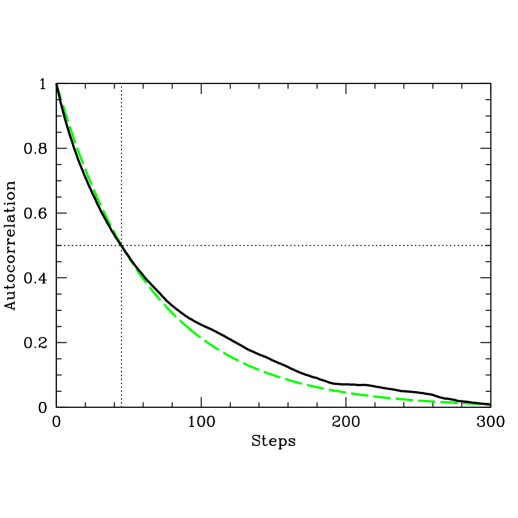
Figure 16: The autocorrelation function (solid curve) for the example in Figure 15 is seen to be approximately fit by an exponential (dashed curve), dropping to 50% at a correlation length of 45 steps as indicated by the dotted lines.

As illustrated in Figure 15, consecutive points ${\bf p}_{i}$, $i=1,...$ of a MCMC are correlated. We quantify this by the dimensionless autocorrelation function $c$, shown for the reionization parameter $\tau$ in Figure 16 and defined by

$$c_{j}\equiv{\langle\tau_{i}\tau_{i+j}\rangle-\langle\tau_{i}\rangle^{2}\over\langle\tau_{i}^{2}\rangle-\langle\tau_{i}\rangle^{2}},$$ (4)

where averages are over the whole chain. The correlation is by definition unity at zero lag, and we define the correlation length as the number of steps over which the correlation drops to 0.5. The figure of merit for a chain is its effective length $N$, defined as the number of steps divided by the correlation length. Since $N$ is roughly speaking the number of independent points, the MCMC technique measures statistical quantities such as the standard deviation $\sigma_{p}$ and the mean $\langle p\rangle$ for cosmological parameters to an accuracy of order $\sigma_{p}/N^{1/2}$. Unless $N\gg 1$, the results are useless and misleading, a problem referred to as insufficient mixing in the MCMC literature Gilks96 .

We attempt to minimize the correlation length by tailoring the jump function to the structure of the likelihood function. Consider first a toy model with a one-dimensional parameter space and a Gaussian likelihood $\L(p)\propto e^{-p^{2}/2}$ and a Gaussian jump function $f(\Delta p)\propto e^{-\Delta p^{2}/2\sigma^{2}}$. What is the best choice of the characteristic jump size $\sigma$? In the limit $\sigma\to\infty$, all jumps will fail; $p_{1}=p_{2}=...$, $c_{j}=1$ for all $j$ and the correlation length becomes infinite. In the opposite limit $\sigma\to 0$, almost all steps succeed and we obtain Brownian motion with the rms value $|p_{i}|\sim\sigma i^{1/2}$, so it takes of order $\sigma^{-2}\to\infty$ steps to wander from one half of the distribution to the other, again giving infinite correlation length. This implies that there must be an optimal jump size between these extremes, and numerical experimentation shows that $\sigma\sim 1$ minimizes the correlation length.

In the multiparameter case, strong degeneracies can cause a huge correlation length if the jump size is chosen independently for each parameter, with the chain taking a very long time to wander from one end of the banana to the other. A clever choice of parameters that reduces degeneracies therefore reduces the correlation length. For this reason, the WMAP team used the parameters suggested by Kosowsky02 , and we do the same with the minor improvement of replacing $A_{s}$ by $A_{p}$ as the scalar normalization parameter as in Knox03 . To minimize the remaining degeneracies, we compute the parameter covariance matrix ${\bf C}\equiv\langle{\bf p}{\bf p}^{t}\rangle-\langle{\bf p}\rangle\langle{\bf p}\rangle^{t}$ from the chain itself, diagonalize it as ${\bf C}={\bf R}{\bf\Lambda}{\bf R}^{t}$, ${\bf R}{\bf R}^{t}={\bf R}^{t}{\bf R}={\bf I}$, ${\bf\Lambda}_{ij}=\delta_{ij}\lambda_{i}^{2}$, and work with the transformed parameter vector ${\bf p}^{\prime}\equiv{\bf\Lambda}^{-1/2}{\bf R}^{t}[{\bf p}-\langle{\bf p}\rangle]$ which has the benign properties $\langle{\bf p}^{\prime}\rangle={\bf 0}$, $\langle{\bf p}^{\prime}{\bf p}^{\prime t}\rangle={\bf I}$. Inspired by the above-mentioned one-dimensional example, we then use the simple jump function $f(\Delta{\bf p}^{\prime})\propto e^{-|\Delta{\bf p}^{\prime}|^{2}/2\sigma^{2}}$. We use $\sigma=1$ for all chains except number 1 in Table 8, where we obtain a shorter correlation length using $\sigma=0.7$. When running our test chains to optimize $f$, we start by guessing a diagonal ${\bf C}$ and after the burn-in, we update our estimates of both ${\bf C}$ and the eigenbasis every 100 steps. A very similar approach is used in other recent MCMC codes, e.g., Lewis02 ; ZahnZalda03 .

The WMAP team perform extensive testing to confirm that their chains are properly mixed Verde03 , and we have followed the WMAP team in using the Gelman and Rubin $R$-statistic GelmanRubin92 to verify that our chains are sufficiently converged and mixed. Indeed, we find that the above-mentioned eigenbasis technique helps further improve the mixing by cutting our correlation length by about an order of magnitude relative to that obtained with the WMAP jump function, hence greatly increasing the effective length of our chains.

A.3 The likelihood function $\L$

For a detailed discussion of how to compute cosmological likelihood functions, see BJK ; Verde03 . Our calculation of $\L({\bf p},{\bf d})$ does little more than combine public software described in other papers, so the details in this brief section are merely of interest for the reader interested in exactly reproducing our results.

The total likelihood $\L$ is simply a product of likelihoods corresponding to the data sets used, e.g., WMAP, SDSS and SN Ia. For the CMB, we compute theoretical power spectra using version 4.3 of CMBfast cmbfast , with both the “RECfast” and “PRECISION” options turned on. We compute the WMAP likelihood corresponding to these spectra using the public software provided by the WMAP team Verde03 . Since this software is designed for physically reasonable models, not for crazy models that may occur during our burn-in, we augment it to produce large negative likelihoods for unphysical models where it would otherwise give negative $\chi^{2}$-values. For some of the WMAP+SDSS chains, we evaluate the WMAP likelihood $\L_{\rm WMAP}$ by fitting a quartic polynomial to $\ln\L_{\rm WMAP}$ from the corresponding WMAP-only chains. For this fit, we replace $\omega_{d}$ by $\omega_{\rm m}$, $\omega_{b}$ by $H_{2}$, ${n_{s}}$ by $H_{3}$ and $A_{p}$ by $A_{*}$ inspired by the normal parameter method of Knox03 . This approach, described in detail in cmbfit , is merely a numerical tool for accelerating the computations, and we verify that it has negligible impact on our results.

When combining non-WMAP CMB data with WMAP, we include the latest band-power detections from Boomerang Ruhl02 (madcap), DASI Halverson01 , MAXIMA Lee01 , VSA VSA02 , CBI (mosaic, even binning) Sievers02 and ACBAR Kuo02 with probing effective multipoles $\l\geq 600$ (where they are collectively more sensitive than WMAP) and $\l\leq 2000$ (to avoid complications related to reported small-scale excess, which may be due to secondary anisotropies or non-CMB effects), which corresponds to the $9+3+3+4+6+9=34$ data points plotted in Figure 17. The pre-WMAP data has been shown to be consistent both internally and with WMAP GriffithsLineweaver03 . We marginalize over the quoted calibration uncertainties of 10% for Boomerang, 4% for MAXIMA and DASI, 5% for CBI, 3.5% for VSA and 10% for ACBAR as well as over quoted beam uncertainties of 15% for Boomerang, 5% for ACBAR and 14% for MAXIMA (this last number provides a good fit to the combined beam and pointing uncertainties for the three measurements used from Table 1 of Lee01 ). We make the approximation that all experiments are uncorrelated with each other and with WMAP, which should be quite accurate both since sample variance correlations are negligible (given their small sky coverage relative to WMAP) and since the wmap errors are dominated by detector noise for $\l\geq 600$. When using non-CMB data without WMAP, we use all 151 pre-WMAP band power measurements compiled in cmblsslens . For the non-WMAP data, we computed the CMB power spectra with the DASh package DASh .

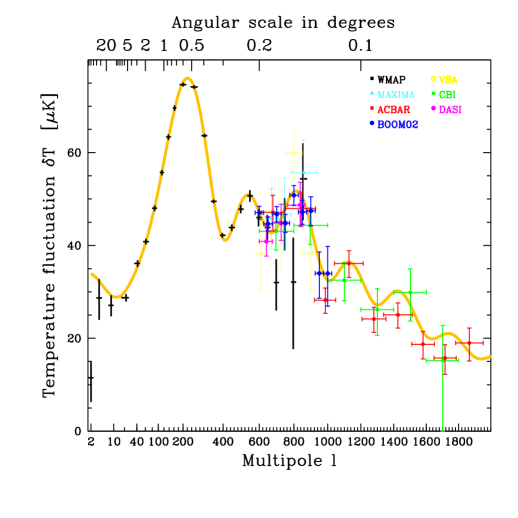
Figure 17: CMB data used. Error bars show do not include the calibration and beam uncertainties that we include as described in the text. Solid curve corresponds to the “vanilla lite” model of equation (2).

For SDSS, we compute the likelihood by fitting $b^{2}$ times the nonlinear power spectrum $P(k)$ to the first 19 band power measurements (for $k<k_{\rm max}\sim 0.2h/$Mpc) using the window functions and likelihood software provided by that paper sdsspower . For more details about the SDSS data, see BlantonTiling ; EisensteinLRGselection ; FukugitaFilters ; GunnCamera ; HoggPt ; PierAstrometry ; SmithPhotometry ; StraussTargetSelection . We compute the nonlinear $P(k)$ using the method and software provided by Smith03 . This software takes the linear power spectrum $P(k)$ as input, and we compute it using the fitting software provided by Novosyadlyj99 for the transfer function, the approximation of Carroll92 for the linear growth factor and the approximation that $P(k)$ is as a product of these two quantities as per equation (C3) from concordance . For $k\mathrel{\hbox to0.0pt{\lower 3.0pt\hbox{$\mathchar 536\relax$}\hss}\raise 2.0pt\hbox{$\mathchar 318\relax$}}0.2$, this typically agrees with CMBfast 4.3 to better than a few percent. In the absence of massive neutrinos ($f_{\nu}=0$), the separability approximation becomes exact and the transfer function fits Novosyadlyj99 become identical to those of Eisenstein & Hu Eisenstein99 .

For SN Ia, we use the 172 redshifts and corrected peak magnitudes compiled and uniformly analyzed by Tonry et al. Tonry03 and compute the likelihood with software kindly provided by John Tonry. This likelihood depends only on $(\Omega_{\Lambda},\Omega_{k},w)$, and is marginalized over the corrected SN Ia “standard candle” absolute magnitude.

A.4 Confidence limits and likelihood plots

All confidence limits quoted in the tables and text of this paper are quantiles, as illustrated in Figure 18. For instance, our statement in Table 3 that $M_{\nu}<1.74$eV at 95% confidence simply means that 95% of the $M_{\nu}$-values in that chain are smaller than $1.74$eV. Similarly, the entry ${n_{s}}=0.972^{+0.041}_{-0.027}$ in the same column means that the distribution of ${n_{s}}$-values has median $0.972$, that erfc$(2^{-1/2})/2\approx 15.87\%$ of the values lie below $0.972-0.027$ and that 15.87% of the values lie above $0.972+0.041$, so that 68.27% lie in the range ${n_{s}}=0.972^{+0.041}_{-0.027}$. There is thus no assumption about the distributions being Gaussian. In a handful of cases involving $r$, $f_{\nu}$ and $M_{\nu}$, the distribution (see Figure 2 for examples) peaks at zero rather than near the median; in such cases, we simply quote an upper limit.

When plotting 1-dimensional distributions $f(p)$ in Figure 2, we fit each histogram to a smooth function of the form $f(p)=e^{P(p)}$ where $P(p)$ is the 6th order polynomial that maximizes the likelihood $\prod_{i=1}^{n}f(p_{i})$ that the points $p_{1},...,p_{n}$ in the chain are drawn from the distribution $f(p)$, subject to the constraint that $\int f(p)dp=1$. We found that these smooth curves visually match the raw histograms extremely well (see Figure 18 for a rather non-Gaussian example) and have the advantage of avoiding both the Poisson jaggedness and the excessive smoothing inherent in a histogram.

Our 2-dimensional contours are plotted where the point density has dropped by $e^{-\Delta\chi^{2}/2}$ from its maximum, where $\Delta\chi^{2}=6.18$ as recommended in §15.6 of NumRecipes . These contours would enclose 95% of the points if the distribution were Gaussian. When computing the point density, there is tradeoff between insufficient smoothing (giving contours dominated by Poisson noise) and excessive smoothing (which artificially broadens the contours, particularly in the narrow direction of a degeneracy banana). We found that this was alleviated by computing the contours in the linearly transformed 2-dimensional space defined in Section A.2 where the covariance matrix is the identity matrix.

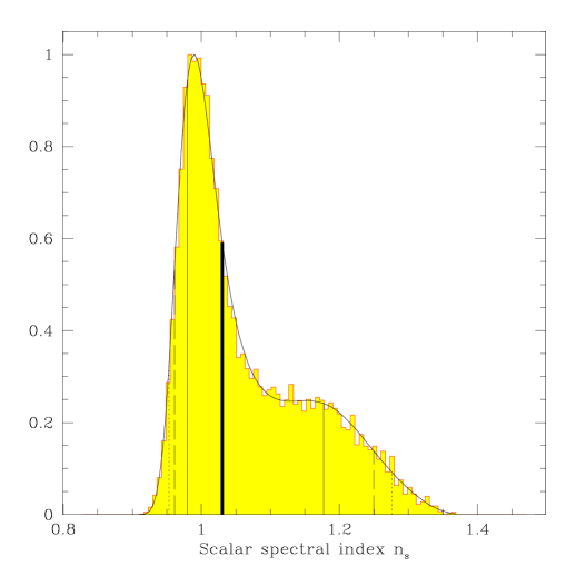
Figure 18: Example of the likelihood fitting technique we use for plotting. The shaded histogram shows the distribution of the 311391 ${n_{s}}$-values from chain 6 in Table 8.. The black curve shows our fit $e^{P({n_{s}})}$ for the 6th order $P({n_{s}})$ maximizing the Poisson likelihood as described in the text. The vertical lines show the quantiles of the distribution that we use to quote confidence intervals: the median (heavy line), the central $68\%$ (between thin solid lines), the central 90% (between dashed lines) and the central 95% (between dotted lines) of the distribution.

References

- (1) C. L. Bennett et al., ApJS, 148, 1 (2003)
- (2) G. Hinshaw et al., ApJS, 148, 135 (2003)
- (3) A. Kogut et al., ApJS, 148, 161 (2003)
- (4) L. Page et al., ApJS, 148, 233 (2003)
- (5) H. V. Peiris et al., ApJS, 148, 213 (2003)
- (6) D. N. Spergel et al., ApJS, 148, 175 (2003)
- (7) L. Verde et al., ApJS, 148, 195 (2003)
- (8) S. Bridle, O. Lahav, J. P. Ostriker, and P. J. Steinhardt, Science, 299, 1532 (2003)
- (9) M. Colless et al., MNRAS, 328, 1039 (2001)
- (10) M. Colless et al., astro-ph/0306581, 2003
- (11) W. J. Percival et al., MNRAS, 327, 1297 (2001)
- (12) J. R. Bond, G. Efstathiou, and M. Tegmark, MNRAS, 291, L33 (1997)
- (13) M. Zaldarriaga, D. Spergel, and U. Seljak, ApJ, 488, 1 (1997)
- (14) Y. Wang, D. N. Spergel, and M. A. Strauss, ApJ, 510, 20 (1999)
- (15) D. J. Eisenstein, W. Hu, and M. Tegmark, ApJ, 518, 2 (1999)
- (16) G. Efstathiou and J. R. Bond, MNRAS, 304, 75 (1999)
- (17) D. G. York et al., Astron.J., 120, 1579 (2000)
- (18) C. Stoughton et al., Astron.J., 123, 485 (2002)
- (19) K. Abazajian et al., Astron.J., 126, 2081 (2003)
- (20) M. Tegmark, M. Blanton, M. A. Strauss, F. S. Hoyle, D. Schlegel, R. Scoccimarro, M. S. Vogeley, D. H. Weinberg, I. Zehavi et al. 2003, ApJ, submitted
- (21) L. Verde et al., MNRAS, 335, 432 (2002)
- (22) X. Wang, M. Tegmark, and M. Zaldarriaga, Phys. Rev. D, 65, 123001 (2002)
- (23) U. Seljak, and M. Zaldarriaga, ApJ, 469, 437 (1996)
- (24) M. Chu, M. Kaplinghat, and L. Knox, ApJ, 596, 725 (2003)
- (25) W. Hu, M. Fukugita, M. Zaldarriaga, and M. Tegmark, ApJ, 549, 669 (2001)
- (26) A. Kosowsky, M. Milosavljevic, and Jimenez R, PRD, 66, 73007 (2002)
- (27) N. Metropolis, A. W. Rosenbluth, M. N. Rosenbluth, A. H. Teller, and E. Teller, J.Chem.Phys., 21, 1087 (1953)
- (28) W. K. Hastings, Biometrika, 57, 97 (1970)
- (29) W. R. Gilks, S. Richardson, and D. J. Spiegelhalter, Markov Chain Monte Carlo in Practice (Chapman & Hall: London, 1996)
- (30) A. Gelman and D. Rubin, Statistical Science, 7, 457 (1992)
- (31) N. Christensen, R. Meyer, L. Knox, and B. Luey, Class. Quant. Grav., 18, 2677 (2001)
- (32) A. Lewis and S. Bridle, PRD, 66, 103511 (2002)
- (33) A. Slosar and M. Hobson, astro-ph/0307219, 2003
- (34) R. E. Smith et al., MNRAS, 341, 1311 (2003)
- (35) J. L. Tonry et al., ApJ, 594, 1 (2003)
- (36) A. Lewis, astro-ph/0310186, 2003
- (37) M. Tegmark, J. Silk, and A. Blanchard, ApJ, 420, 484 (1994)
- (38) E. W. Kolb and M. S. Turner, The Early Universe (Addison Wesley: New York, 1990)
- (39) S. M. Carroll, W. H. Press, and E. L. Turner, ARA&A, 30, 499 (1992)
- (40) A. J. S Hamilton, MNRAS, 322, 419 (2000)
- (41) R. H. Cyburt,B. D. Fields, and K. A. Olive, Phys. Lett. B, 567, 227 (2003)
- (42) A. Cuoco, F. Iocco, Mangano G, Miele G, O. Pisanti, and P. D. Serpico, astro-ph/0307213, 2003
- (43) Coc A, E. Vangioni-Flam, P. Descouvemont, Adahchour A, , and C. Angulo 2003, in Tours Symposium on Nuclear Physics V
- (44) S. Burles and D. Tytler, ApJ, 499, 699 (1998)
- (45) P. N. Walker et al., ApJ, 376, 51 (1991)
- (46) M. S. Smith, L. H. Kawano, and R. A. Malaney, ApJS, 85, 219 (1993)
- (47) M. Tegmark, M. Zaldarriaga, and A. J. S Hamilton, Phys. Rev. D, 63, 43007 (2001)
- (48) S. S. McGaugh, ApJL, 541, L33 (2000)
- (49) W. L. Freedman et al., ApJ, 553, 47 (2001)
- (50) N. A. Bahcall and P. Bode, ApJ, 588, L1-L4 (2003)
- (51) E. Pierpaoli, D. Scott, and M. White, MNRAS, 325, 77 (2001)
- (52) S. W. Allen, R. W. Schmidt, A. C. Fabian, and H. Ebeling, MNRAS, 342, 287 (2001)
- (53) M. L. Brown et al., MNRAS, 341, 100 (2003)
- (54) H. Hoestra, H. K. C Yee, and M. D. Gladders, ApJ, 577, 595 (2002)
- (55) D. Bacon, R. Massey, A. Refregier , and R. Ellis, MNRAS, 344, 673 (2003)
- (56) A. Voevodkin and A. Vikhlinin, astro-ph/0305549, 2003
- (57) E. Pierpaoli, S. Borgani, D. Scott, and M. White, MNRAS, 342, 163 (2003)
- (58) P. Schuecker, H. Böhringer, C. A. Collins, and L. Guzzo, Astro. Astrophys., 398, 867 (2003)
- (59) P. T. P Viana, S. T. Kay, A. R. Liddle, O. Muanwong, and P. A. Thomas, 346;319, 2003MNRAS
- (60) U. Seljak, MNRAS, 337, 769 (2002)
- (61) T. H. Reiprich and H. Boehringer, ApJ, 567, 716 (2002)
- (62) S. Borgani et al., ApJ, 561, 13 (2001)
- (63) C. Heymans, M. Brown, A. Heavens, K. Meisenheimer, A. Taylor, and C. Wolf, astro-ph/0310174, 2003
- (64) M. Jarvis et al., AJ, 125, 1014 (2003)
- (65) A. Refregier, J. Rhodes , and E. J. Groth, ApJ, 572, L131 (2002)
- (66) Waerbeke. L. van et al., A&A, 393, 369 (2002)
- (67) T. Hamana et al., ApJ;597;98, 2003
- (68) C. R. Contaldi, H. Hoekstra, and A. Lewis, PRL, 99, 221303 (2003)
- (69) J. P. Ostriker, K. Nagamine, R. Cen, and M. Fukugita, ApJ, 597, 1 (2003)
- (70) O. Lahav et al., MNRAS, 333, 961 (2002)
- (71) A. Linde, JCAP, 305, 2 (2003)
- (72) G. Efstathiou, MNRAS, 343, L95 (2003)
- (73) A. Vilenkin and S. Winitzki, Phys. Rev. D, 55, 548 (1997)
- (74) M. Tegmark and M. J. Rees, ApJ, 499, 526 (1998)
- (75) A. D. Linde, Phys. Lett. B, 351, 99 (1995)
- (76) B. M. S Hansen et al., ApJ, 574, L155 (2002)
- (77) C. H. Lineweaver, Science, 284, 1503 (2000)
- (78) M. White, ApJ, 506, 495 (1998)
- (79) S. Dodelson, hep-ph/0309057, 2003
- (80) S. Dodelson, W. H. Kinney, and E. W. Kolb, PRD, 56, 3207 (1997)
- (81) A. R. Liddle and D. H. Lyth, Cosmological Inflation and Large-Scale Structure (Cambridge Univ. Press: Cambridge, 2000)
- (82) D. H. Lyth and A. A. Riotto, Phys. Rep., 314, 1 (1999)
- (83) W. H. Kinney, E. W. Kolb, A. Melchiorri, and A. Riotto, hep-ph/0305130, 2003
- (84) A. R. Liddle and A. J. Smith, PRD, 68, 061301 (2003)
- (85) D. Wands, New Astron. Reviews, 47, 781 (2003)
- (86) A. R. Liddle and S. M. Leach, PRD, 68, 103503 (2003)
- (87) L. Hui and S. Dodelson, PRL, 91, 131301 (2003)
- (88) A. D. Linde, Particle Physics and Inflationary Cosmology (Harwood: Chur, Switzerland, 1990)
- (89) B. Kyae and Q. Shafi, JHEP, 311, 36 (2003)
- (90) J. E. Lidsey and R. Tavakol, Phys. Lett. B, 575, 157 (2003)
- (91) G. Efstathiou, 2003, MNRAS, 346;L26 (2003)
- (92) A. de Oliveira-Costa, M. Tegmark, M. Zaldarriaga, and A. J. S Hamilton, astro-ph/0307282, 2003
- (93) T. J. Pearson et al., ApJ, 556, 574 (2003)
- (94) U. Seljak, P. McDonald, and A. Makarov, MNRAS, 342, L79 (2003)
- (95) W. Hu, D. J. Eisenstein, and M. Tegmark, PRL, 79, 3806 (1998)
- (96) S. Hannestad, JCAP, 05, 004 (2003)
- (97) O. Elgaroy and O. Lahav, JCAP, 0304, 004 (2003)
- (98) S. Bashinsky and Seljak U, astro-ph/0310198, 2003
- (99) S. Hannestad, astro-ph/0310133, 2003
- (100) S. King, hep-ph/0310204, 2003
- (101) A. D. Dolgov, S. H. Hansen, S. Pastor, S. T. Petcov, G. G. Raffelt, and D. V. Semikoz, Nucl. Phys. B, 632, 363 (2002)
- (102) K. N. Abazajian, J. F. Beacom, and N. F. Bell, PRD, 66, 013008 (2002)
- (103) Y. Y. Wong, PRD, 66, 025015 (2002)
- (104) E. T. Kearns, hep-ex/0210019, 2002
- (105) S. N. Ahmed et al., nucl-ex/0309004, 2003
- (106) J. N. Bahcall, JHEP, 0311, 004 (2003)
- (107) P. Di Bari, PRD, 65, 043509 [Addendum-ibid. D 67, 127301 (2003)] (2002)
- (108) K. N. Abazajian, Astropart. Phys., 19, 303 (2003)
- (109) S. W. Allen, R. W. Schmidt, and S. L. Bridle, MNRAS, 346, 593 (2003)
- (110) A. Melchiorri, L. Mersini, C. J. Odman, and M. Trodden, PRD, 68, 043509 (2002)
- (111) T. Barreiro, M. C. Bento, N. M. C Santos, and A. A. Sen, Phys. Rev. D, 68, 043515 (2003)
- (112) S. DeDeo, R. R. Caldwell, and P. J. Steinhardt, PRD, 67, 103509 (2003)
- (113) R. R. Caldwell and M. Doran, astro-ph/0305334, 2003
- (114) R. R. Caldwell, M. Kamionkowski, and N. N. Weinberg, Phys. Rev. Lett, 91, 071301 (2003)
- (115) R. R. Caldwell, M. Doran, C. M. Mueller, G. Schaefer, and C. Wetterich, ApJ, 591, L75-L78 (2003)
- (116) A. B. Balakin, D. Pavon, D. J. Schwarz, and W. Zimdahl, New J.Phys., 5, 85 (2003)
- (117) J. Weller and A. M. Lewis, MNRAS, 346, 987; (2003)
- (118) M. Kunz, P. S. Corasaniti, Parkinson D, and E. J. Copeland, astro-ph/0307346, 2003
- (119) R. Easther, astro-ph/0308160, 2003
- (120) M. Tegmark and A. Vilenkin, astro-ph/0304536, 2003
- (121) Y. Wang and P. Mukherjee, astro-ph/0312192, 2003
- (122) U. Alam, V. Sahni, T. D. Saini, and A. A. Starobinsky, astro-ph/0311364, 2003
- (123) G. Rocha et al., astro-ph/0309211, 2003
- (124) R. Trotta and S. H. Hansen, astro-ph/0306588, 2003
- (125) G. Huey, R. H. Cyburt, and B. D. Wandelt, astro-ph/0307080, 2003
- (126) P. Crotty, J. Garcia-Bellido, J. Lesgourgues, and A. Riazuelo, PRL, 91, 171301 (2003)
- (127) S. L. Bridle, A. M. Lewis, J. Weller, and G. Efstathiou, MNRAS, 342, L72 (2003)
- (128) S. Hannestad, astro-ph/0311491, 2003
- (129) L. Knox, R. Scoccimarro, and S. Dodelson, PRL, 81, 2004 (1998)
- (130) Y. Song-S and L. Knox, Phys. Rev. D, 68, 043518 (2003)
- (131) S. Boughn and R. Crittenden, astro-ph/0305001, 2003
- (132) M. Nolta et al., astro-ph/0305097, 2003
- (133) P. Fosalba and E. Gaztanaga, astro-ph/0305468, 2003
- (134) P. Fosalba, E. Gaztanaga, and F. Castander, ApJL, 597, L89 (2003)
- (135) R. Scranton et al., astro-ph/0307335, 2003
- (136) N. Afshordi, Y. Loh, and M. A. Strauss, astro-ph/0308260, 2003
- (137) W. Hu, ApJ, 522, L21 (1999)
- (138) M. Kaplinghat, L. Knox, and Y. S. Song, astro-ph/0303344, 2003
- (139) K. N. Abazajian and S. Dodelson, PRL, 91, 041301 (2003)
- (140) T. Budavari et al., ApJ, 595, 59 (2003)
- (141) N. A. Bahcall et al., ApJ, 585, 182 (2003)
- (142) I. Zehavi et al., ApJ, 571, 172 (2002)
- (143) P. Fischer et al., AJ, 120, 1198 (2000)
- (144) C. H. Lineweaver, ApJL, 505, L69 (1998)
- (145) M. Tegmark, ApJL, 514, L69 (1999)
- (146) A. E. Lange et al., PRD, 63, 42001 (2001)
- (147) O. Zahn and M. Zaldarriaga, PRD, 67, 63002 (2003)
- (148) J. R. Bond, A. H. Jaffe, and L. E. Knox, ApJ, 533, 19 (2000)
- (149) H. Sandvik, M. Tegmark, X. Wang, and M. Zaldarriaga, astro-ph/0311544, 2003
- (150) J. E. Ruhl et al., astro-ph/0212229, 2002
- (151) N. W. Halverson et al., ApJ, 568, 38 (2002)
- (152) A. T. Lee et al., ApJ, 561, L1 (2001)
- (153) A. C. Taylor et al., MNRAS, 341, 1066 (2003)
- (154) J. L. Sievers et al., ApJ, 591, 599 (2003)
- (155) C. L. Kuo et al., astro-ph/0212289, 2002
- (156) L. M. Griffiths and C. H. Lineweaver, astro-ph/0311373, 2003
- (157) X. Wang, M. Tegmark, B. Jain, and M. Zaldarriaga, astro-ph/0212417, 2002
- (158) M. Kaplinghat, L. Knox, and C. Skordis, ApJ, 578, 665 (2002)
- (159) M. R. Blanton, R. H. Lupton, F. M. Maley, N. Young, I. Zehavi, and J. Loveday, AJ, 125, 2276 (2003)
- (160) D. J. Eisenstein et al., AJ, 122, 2267 (2001)
- (161) M. Fukugita, T. Ichikawa, J. E. Gunn, M. Doi, K. Shimasaku , and D. P. Schneider, Astron. J., 111, 1748 (1996)
- (162) J. E. Gunn, M. A. Carr, C. M. Rockosi, M. Sekiguchi et al., Astron. J., 116, 3040 (1998)
- (163) D. W. Hogg, D. P. Finkbeiner, D. J. Schlegel, and J. E. Gunn, AJ, 122, 2129 (2001)
- (164) J. R. Pier et al., AJ, 125, 1559 (2003)
- (165) J. A. Smith et al., AJ, 123, 2121 (2002)
- (166) M. A. Strauss et al., AJ, 124, 1810 (2002)
- (167) B. Novosyadlyj, R. Durrer, and Lukash V N, A&A, 347, 799 (1999)
- (168) D. J. Eisenstein and W. Hu, ApJ, 511, 5 (1999)
- (169) W. H. Press et al., Numerical Recipes, 2nd ed. (Cambridge Univ. Press: Cambridge, 1992)