The Diverse Nature of Intrinsic Absorbers in AGNs

Abstract

Intrinsic absorbers are significant components of AGN environments that provide valuable information and interesting challenges. We present a very brief (and biased, and sometimes speculative) overview of intrinsic absorbers from the perspective of different absorption line classes. We also discuss ways of addressing and learning from the “problem” of partial coverage of the background light source, with some examples based on new high-resolution rest-frame UV spectra of quasars.

University of Florida, Dept. of Astronomy, 211 Bryant Space Science Center, Gainesville, FL 32653-2055, USA

American University of Science & Technology, Dept. of Mathematics, Zahle, Lebanon

1. Introduction: Why Study Intrinsic Absorbers?

Let us start by defining “intrinsic” absorption in terms of gas that is (or was) part of the overall AGN/host galaxy environment. This definition excludes only very distant, cosmologically intervening material, such as intergalactic clouds or unrelated galaxies. It reminds us that, especially in quasar studies, absorption can occur in a wide range of environments. The rich variety of intrinsic absorbers yields numerous diagnostics of both the AGN phenomenon and the AGN–host galaxy connection. A short list of reasons for studying intrinsic absorption might include the following.

$\bullet$ Intrinsic absorbers are a fundamental component of AGN environments. They are common in Type I (broad emission line) AGNs (see below), and might be ubiquitous if the absorbing gas fills only part of the sky as seen from the central continuum source. In addition, the amounts of absorbing gas might be enormous — rivalling or exceeding the mass in the broad emission line region.

$\bullet$ Many intrinsic absorbers are involved in AGN outflows. The flows are driven by the same accretion processes that feed the central super-massive black hole (SMBH) and fuel other AGN energetics. The need for accreting matter to expel angular momentum probably means that the wind mass loss rates, $\dot{M}_{wind}$, are directly proportional to the mass accretion rate, $\dot{M}_{acc}$.

$\bullet$ The relationship between outflow and accretion also implies that intrinsic absorbers are connected to the basic physics of SMBH growth and AGN evolution.

$\bullet$ Intrinsic absorption that occurs far from the AGN might uniquely measure a variety of regions in the host galaxies, such as the interstellar medium, gas streams in galactic halos, or galactic super-winds driven by starburst activity.

$\bullet$ The metal abundances in high-redshift intrinsic absorbers can provide unique constraints on the amount of star formation and the overall maturity of young galactic or proto-galactic nuclei.

$\bullet$ The metal-rich gas expelled by high-redshift AGNs might be a significant source of metal “pollution” to the intergalactic medium at early cosmic times.

In this brief review, we focus on a few issues regarding absorption line classification, the relationships between classes, and the implications of partial coverage of the background light source(s). See also the reviews by Crenshaw, Kraemer, & George (2003), Hamann (2000), Hamann & Ferland (1999), and the ASP conference series volumes (128 and 255) devoted to AGN mass loss.

2. Absorption Line Classes

AGN absorption lines are classified empirically by the full width at half minimum (FWHM) of their profiles. The class definitions necessarily evolve as we encounter new phenomena and assimilate different measurement schemes. Nonetheless, standardized classes are essential. The main classes are the “narrow” absorption lines (NALs), the “broad” absorption lines (BALs), and a catch-all intermediate class called the mini-BALs.

BALs are blueshifted from the systemic (emission line) redshift by as much as $\sim$0.2$c$, and clearly form in winds form the central engine. Weymann et al. (1991) introduced a “BAL-nicity” index to define this class. Hall et al. (2002) proposed a less restrictive index to include a wider range of line widths. We strongly advocate the use of quantitative indices, but a reasonable starting point for casual conversation is that BALs have continuous absorption over $>2000$ km/s, with at least some portion of the profile having a velocity shift $v>2000$ km/s compared to systemic. BALs are further divided into subclasses according to the degree of ionization apparent in the lines. “HiBALs” have nominally SiIV $\lambda\lambda$1394,1403 and CIV $\lambda\lambda$1548,1551 (or perhaps CIII $\lambda$977) as their lowest ionization lines. “LoBALs” include lower ionization stages, such as MgII $\lambda\lambda$2796,2804. “FeLoBALs” have more extreme low-ionzation regions that produce excited-state absorption in FeII (requiring densities $n_{e}\mathrel{\hbox{\hbox to0.0pt{\hbox{\lower 4.0pt\hbox{$\sim$}}\hss}\hbox{$>$}}}10^{5}$ cm^-3).

A useful (but physically arbitrary) definition of NALs is that they are narrow enough not to blend important UV doublets, e.g., the CIV pair with separation $\sim$500 km/s. Thus we require FWHM $<200$ to 300 km/s. NALs with velocity shifts $v<5000$ km/s from systemic are also call “associated” absorption lines (AALs) because of their plausible physical relationship to the AGN. No one has yet sub-divided AALs into HiAALs and LoAALs analogous to the BALs, but it would be interesting to compare sub-classes based on these properties.

Mini-BALs have FWHMs intermediate between the NALs and BALs. They appear at the same range of blueshifted velocities as the BALs, and they also clearly form in AGN outflows. Examples of high-velocity mini-BALs can be found in Jannuzi et al. (1996) and Hamann et al. (1997a). For the BALs, see Weymann et al. (1991), Reichard et al. (2003), and Hall et al. (2002). For the AALs, see Foltz et al. (1986) and Ganguly et al. (1999). See also the reviews cited above.

Figure 1 lists the major absorption line classes along with some properties and speculation that we will describe below. The detection frequencies given in the figure are our own educated guesses, except for the quasar AALs (G. Richards, priv. comm.), Seyfert 1 AALs (Crenshaw et al. 1999), and the HiBALs and LoBALs (Weymann et al. 1991, Reichard et al. 2003). Note that we list all Seyfert 1 absorbers as NALs, even though some may be considered mini-BALs.

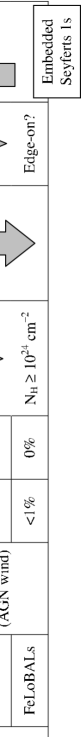
Figure 1.: Absorption line classes and characterictics.

3. Identifying Intrinsic NALs

Quasar NALs are known to form in a wide range of environments, from outflows like the BALs to unrelated gas or galaxies at large (cosmologically significant) distances from the AGN (Weymann et al. 1979). NALs in low-redshift Seyfert 1 galaxies might be almost exclusively intrinsic, but there is still a range of possible locations within the global AGN/host galaxy environment. An important goal, therefore, is to identify the intrinsic NALs and locate the absorbing regions with respect to the AGNs/host galaxies. One strategy is to examine the probabilities. For example, quasars have an over-density of NALs near the emission redshift, i.e., more than expected for a random distribution of cosmologically intervening material (Weymann et al. 1979, Foltz et al. 1986). Others have noted that the presence and/or strengths of NALs correlate with AGN properties such as luminosity, radio-loudness, and radio lobe orientation (Wills et al. 1995, Richards et al. 1999, Richards 2001). These relationships imply that a substantial fraction of quasar AALs ($>$50%), and probably some of the highly blueshifted ($v>5000$ km/s) NALs, are intrinsic to quasars.

We can also examine individual absorbers to look for i) absorption line variability, ii) profiles that are broad and smooth compared to thermal speeds, iii) partial line-of-sight coverage of the background light source, and iv) high gas densities based on excited-state absorption lines (see below, also Tripp, Lu, & Savage 1996, Hamann et al. 1997b, 2001, Barlow & Sargent 1997, Ganguly et al. 1999, Narayanan & Hamann 2003). These characteristics often appear together and suggest an intrinsic origin because they are most easily understood in terms of the dense and dynamic environments near AGNs.

4. Absorber Trends & Characteristics

Brandt, Laor, & Wills (2000) showed that the strengths of intrinsic absorption lines (e.g., $W_{\lambda}$(CIV)) correlate roughly with the amount of X-ray absorption. Moreover, the column densities derived for the X-ray absorbers are much larger than earlier estimates from the UV lines, to the point where some BAL quasars have Thompson thick X-ray absorbers with $N_{H}\mathrel{\hbox{\hbox to0.0pt{\hbox{\lower 4.0pt\hbox{$\sim$}}\hss}\hbox{$>$}}}10^{24}$ cm^-2 (Hamann 1998, Gallagher et al. 1999, Mathur et al. 2000, Arav et al. 2002). In some Seyfert 1 galaxies (e.g., Kaspi et al. 2002) we know that the X-ray absorbing gas is outflowing at modest speeds with the UV line absorbers. It would be more problematic for models invoking radiative acceleration if the large X-ray columns in BAL quasars turn out to be outflowing at BAL speeds (Hamann 1998). In any case, we have an expectation that mass loss rates increase generally with line strength, as shown in Figure 1.

Other studies suggest that, in very rough terms, the amount of reddening, the percent polarization, and perhaps the IR luminosities are all nominally higher in BAL quasars and may increase toward lower ionizations through the BAL class (Weymann et al. 1991, Schmidt & Hines 1999, Brotherton et al. 2002, Hall et al. 2002, Richards et al. 2003, Reichard et al. 2003, and refs. therein). It is not known if these tendencies extend to the mini-BALs or AALs.

5. Evolution & Orientation

AGN evolution is something of a holy grail because we know almost nothing about it. Unlike stars and galaxies, we have yet to identify “young” or “old” AGNs. It has been suggested that the FeLoBAL and LoBAL quasars represent a young phase because their enormous column densities, low ionizations, and reddening might be signatures of an energetic AGN that is still partially enshrouded in its dusty parental environment (Voit, Weymann, & Korista 1993, Gregg et al. 2000, Brotherton et al. 2002, and refs. therein). Perhaps this evolutionary path continues through the BALs to the mini-BAL and AAL stages as the outflows gradually weaken (Figure 1). However, orientation probably also plays an important role. Most models have BAL winds rising up out of the accretion disk and flowing close the the disk plane (Murray et al. 1995, Proga, Stone, & Kallman 2000). Viewing angles close to the disk plane should plausibly lead to larger absorption column densities, detections of lower ionization stages, and perhaps increased reddening and polarization (Schmidt & Hines 1999, Elvis 2000). Similar arguments may apply to the AALs (Wills et al. 1995). It seems likely that orientation and evolution both contribute to differences between the absorber classes.

One observational difficulty is that AGN lifetimes are short compared to their host galaxies, so we cannot argue that young/old AGNs reside in young/old galaxies. In particular, AGN luminosities, $L$, are related to the mass accretion rate onto the central SMBH, $\dot{M}_{acc}$, by an efficiency factor, $\eta$. The luminosities are also some fraction, $\gamma$, of the theoretical Eddingtion limit, $L_{edd}$, such that

$$L\ \approx\ \eta\dot{M}_{acc}\,c^{2}\ \approx\ \gamma L_{edd}\ \approx\ (1.5\times 10^{46})\;\gamma M_{8}~{}~{}~{}({\rm ergs/s})$$ (1)

where $M_{8}$ is the SMBH mass in units of $10^{8}$ M_⊙. If we adopt standard values of $\eta=0.1$ and $\gamma=0.5$, and we assume the lifetime of the bright AGN phase is the time needed for the last doubling of the SMBH mass, then we derive a nominal lifetime of $\sim$$6\times 10^{7}$ yr (see also Ferrarese 2002 and refs. therein).

These lifetimes are also short compared to the duration of the main quasar epoch, for example, the $\sim$$5\times 10^{9}$ yrs elapsed from redshifts 4 to 1. Therefore, we cannot expect to find exclusively young/old AGNs at high/low redshifts. However, we can use the fact that the AGN population is growing rapidly at redshifts $z>3$. At these redshifts, there are more AGNs being created “now” than in the past, so there should be more young AGNs than old ones. Conversely, at $z\mathrel{\hbox{\hbox to0.0pt{\hbox{\lower 4.0pt\hbox{$\sim$}}\hss}\hbox{$<$}}}1$ the AGN population is in rapid decline and there should be more old than young AGNs. The strength of this young versus old signature depends mainly on the slope of the relation between AGN co-moving number density and time. The signature might be strong enough to study age-related trends with redshift in large databases such as the SDSS. We should also keep in mind that the truly youngest AGNs (preceding quasars and having low SMBH masses) will be found among the least luminous sources, perhaps as heavily enshrouded Seyfert 1-like nuclei in dusty starburst galaxies (Figure 1).

6. Column Densities & Partial Coverage

Column density is one of the most critical parameters in intrinsic absorber studies. If we have high resolution spectra, e.g., of absorption lines, we can derive the column density at each velocity shift, $N_{v}$, from the optical depth profile, $\tau_{v}$,

$$N_{v}\ =\ {{m_{e}c}\over{\pi e^{2}f\lambda}}\;\tau_{v}$$ (2)

where $\lambda$ is the line wavelength and $f$ is the oscillator strength. In principle, this analysis is straightforward. In practice, there can be observational and other limitations. There is also a simple question we should consider, which is, what do we mean by “the column density” in a particular ion?

If you walk into a room full of astronomers, even AGN astronomers, and start talking about inhomogeneous absorbing media and partial coverage of the background light source, you will see some eyes roll back in their heads while others look longingly for relief at the clock on the wall. Nonetheless, we keep talking because we believe partial coverage is a fundamental problem that needs to be addressed right now in studies of intrinsic absorption. The problem is more common and probably more insidious than we previously believed. Continuing progress on the big goals outlined in §1 requires a better understanding of the partial coverage issue.

The simplest situation is homogeneous partial coverage (HPC), where the absorber has a constant optical depth across the projected area of an extended emission source. The essential geometry is illustrated in Figure 2a. For simplicity, we assume that the emission source has a constant intensity, $I_{o}$, across its projected area. If $\tau_{v}$ is the optical depth through the absorber at a given velocity shift, and $C_{f}(v)$ is the fraction of the emitting area covered by the absorber (with $0\leq C_{f}(v)\leq 1$), then the measured intensity is a spatial average given by,

$${{I(v)}\over{I_{o}(v)}}\ =\ 1-C_{f}(v)+C_{f}(v)\,e^{-\tau_{v}}$$ (3)

If we measure two lines with a known ratio of optical depths, as in a doublet, then we can solve for the two unknowns, $C_{f}(v)$ and $\tau_{v}$, using the two equations for the measured intensities (Barlow & Sargent 1997, Hamann et al. 1997b, Ganguly et al. 1999).

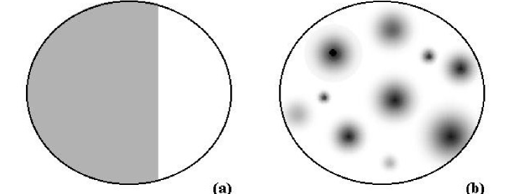
Figure 2.: Skematic illustrations of homogeneous (a) and inhomogeneous (b) partial coverage. The white oval areas represent an extended light source. The shaded regions indicate overlying absorption.

There is growing evidence that the reality is not like Figure 2a, but more like Figure 2b — where the absorber has a range of optical depths across the projected area of the emission source(s). We call this situation inhomogeneous partial coverage (IPC, see deKool et al. 2002, Sabra & Hamann 2003). The evidence for IPC absorbers comes from derived coverage fractions that depend on velocity and, at a given velocity, on the ionization and/or line strength (i.e., true optical depth, see below, also Barlow et al. 1997, Hamann et al. 2001, Arav et al. 2002, and refs. therein). In an IPC cloud distribution (Figure 2b), strong transitions in abundant ions can have $\tau_{v}\mathrel{\hbox{\hbox to0.0pt{\hbox{\lower 4.0pt\hbox{$\sim$}}\hss}\hbox{$>$}}}1$ over a larger area, leading to larger derived coverage fractions. Similarly, low ionization species might have lower coverage fractions if they are concentrated in the smaller, denser regions.

In general, there is a 2-dimensional optical depth structure, $\tau_{v}(x,y)$, in front of an extended emission source with intensities, $I_{o}(x,y,v)$, where $x$ and $y$ are the spatial coordinates. The observed intensity at each velocity shift is the $I_{o}$-weighted average of $e^{-\tau_{v}(x,y)}$,

$$I(v)\ =\ \int\int I_{o}(x,y,v)\;e^{-\tau_{v}(x,y)}\;{{dxdy}\over{A}}$$ (4)

where $A=\int dxdy$ is the total projected area of the emission source (deKool et al. 2002, Sabra & Hamann 2003). deKool et al. (2002) constructed hypothetical $\tau_{v}(x,y)$ distributions and showed how they can affect measured line strengths. They also showed that any $\tau_{v}(x,y)$ can be represented by an equivalent 1-dimensional $\tau_{v}(x)$ without loss of generality. Sabra & Hamann (2003) extended the pioneering work of deKool et al. by i) considering a wider range of $\tau_{v}(x)$ possibilities, ii) showing that even in complex IPC situations we can use measured doublets (or multiplets) to estimate the $\tau_{v}(x)$ shape, and iii) comparing the results of IPC and HPC doublet analyses.

Figure 3 shows one hypothetical $\tau_{v}(x,y)$ distribution composed of overlapping “clouds,” each with a gaussian optical depth spatial profile (see Sabra & Hamann 2003). Also shown is the equivalent 1-dimensional $\tau_{v}(x)$. We use this optical depth distribution to calculate intensities for an absorption line doublet. As in the HPC analysis, the doublet intensities provide two equations from which we can derive two unknowns. But here we adopt a simple functional form for the optical depths, such as the power law $\tau_{v}(x)=\tau_{max}\;x^{a}$, and then solve for $\tau_{max}$ and the “shape” parameter $a$. The results are shown in Figure 3. The power law provides a close but imperfect match to the input $\tau_{v}(x)$ because the input was not a power law. To do better, e.g., in the analysis of real AGN lines, we need theoretical guidance on what functional forms of $\tau_{v}(x)$ are appropriate. It would also help to measure sets of $\geq$3 lines with known optical depth ratios, e.g., in multiplets, to obtain more constraints on $\tau_{v}(x)$.

Figure 3.: Left panel: A synthetic $\tau_{v}(x,y)$ distribution. Right panel: The equivalent $\tau_{v}(x)$ (solid line) plus the best solutions from a doublet analysis assuming a power law $\tau_{v}(x)=\tau_{max}\;x^{a}$ (dotted line) and several other assumed $\tau_{v}(x)$ shapes, including a step function HPC scenario (long-dash line). From Sabra & Hamann (2003).

Finally, we return to the question of what we mean by “the optical depth” or “the column density” in a given feature. Are there single values of these parameters that are meaningful in an IPC environment, e.g., that we can use in a simple ionization/abundance analysis? The answer is probably yes. The input $\tau_{v}(x,y)$ distribution in Figure 3 has a spatially averaged optical depth of $\tau^{avg}_{IPC}\approx 1.2$. The HPC doublet analysis applied to the line intensities emerging through that distribution yields $\tau^{avg}_{HPC}\approx 1.1$. Sabra & Hamann (2003) performed many such experiments. We found that $\tau^{avg}_{IPC}/\tau^{avg}_{HPC}\approx 1$ to within $\sim$30% or so, as long as the input $\tau_{v}(x,y)$ does not contain spatially narrow “spikes.” Such spikes (very large optical depths over a small coverage area) can profoundly affect the average optical depth while having little impact on the observed intensities. Therefore, even with potentially complex IPC absorbers, we can use spatially averaged optical depths derived from the HPC analysis to obtain spatially averaged estimates of the column densities, ionization, abundances, etc.

7. Applications to Real Data

We obtained (with our collaborators T. Barlow, E.M. Burbidge, & V. Junkkarinen) high-resolution spectra of a sample of AAL quasars using the HIRES spectrograph at the Keck 10 m telescope. The quasars have redshifts of order 2, allowing us to measure absorption lines in the rest-frame UV. Figure 4 shows line profiles for several doublets in two of these quasars. The HPC doublet analysis shows that these lines are optically thick at all velocities, while velocity-, ion-, and line-dependent coverage fractions determine the line strengths and profiles (see also Barlow et al. 1997, Arav et al. 2002, and refs. therein). Each individual line (or velocity component) probably does not correspond to a single entity we might call a “cloud” in the absorber. These features will provide only lower limits on the ionic column densities. This situation seems to be common for intrinsic quasar NALs with FWHMs $\mathrel{\hbox{\hbox to0.0pt{\hbox{\lower 4.0pt\hbox{$\sim$}}\hss}\hbox{$>$}}}$ 100 km/s. However, narrower quasar NALs appear to have typically $C_{f}(v)\approx 1$, with each distinct velocity component corresponding to a distinct cloud. This simpler circumstance can yield more reliable column densities and abundances (we find typically $Z\mathrel{\hbox{\hbox to0.0pt{\hbox{\lower 4.0pt\hbox{$\sim$}}\hss}\hbox{$>$}}}$ Z_⊙).

Figure 4.: AAL doublet profiles in CIV, NV $\lambda\lambda$1238,1243, and SiIV in two quasars at redshift $z\sim 2$. The velocities are relative to the broad emission lines. The solid/dotted curves represent the short/long wavelength doublet components, which all have inherently 2/1 optical depth ratios. Derived values of $1-C_{f}(v)$  (large dots) indicate that the lines are optically thick ($\tau_{v}>3$) and velocity-dependent coverage determines each line’s strength and profile. (Noise in the data and overlap with unrelated lines sometimes leads to spuriously low $1-C_{f}(v)$ results, e.g., in SiIV in PG 0935+417.)

References

Arav, N., Korista, K.T., & deKool, M. 2002, ApJ, 566, 699

Barlow, T. A., & Sargent, W. L. W. 1997, AJ, 113, 136

Barlow, T. A., Hamann, F., & Sargent, W. L. W. 1997, in ASP Conf. Series, 128, Mass Ejection From AGN, ed. R. Weymann, I. Shlosman, & N. Arav, 13

Brotherton, M.S., Croom, S.M., De Breuck, C., Becker, R.H., & Gregg, M.D. 2002, AJ, 124, 2575

Crenshaw, D.M., Kraemer, S.B., Boggess, A., Stephen, P., Mushotzky, R.F., & Wu, C.-C. 1999, ApJ, 516, 750

Crenshaw, D.M., Kraemer, S.B., & George, I.M. 2003, ARA&A, 41, 117

deKool, M., Korista, K.T., & Arav, N. 2002, ApJ, 580, 54

Elvis, M. 2000, ApJ, 545, 63

Ferrarese, L. 2002, in Current High Energy Emission Around Black Holes, ed. C.-H. Lee (Singapore: World Scientific) (astro-ph/0203047)

Foltz, C.B, Weymann, R.J., Peterson, B.M., Sun, L., Malkan, M.A., & Chaffee, F.H. 1986, ApJ, 307, 504

Gallagher, S.C., Brandt, W.N., Sambruna, R.M., Mathur, S., & Yamasaki, N. 1999, ApJ, 519, 549

Ganguly, R., Eracleous, M., Charlton, J.C., & Churchill, C.W. 1999, AJ, 117, 259

Hall, P.B., et al. 2002, ApJS, 141, 267

Hamann F. 1998, ApJ, 500, 798

Hamann, F. 2001, in Encyclopedia of Astronomy & Astrophysics, (Institute of Physics), 1079  (astro-ph/9911505)

Hamann F., Barlow, T.A., Cohen, R.D., Junkkarinen, V., Burbidge, E.M., 1997a, in ASP Conf. Ser., 128, Mass Ejection from Active Galactic Nuclei, ed. N. Arav, I. Shlosman, & R.J. Weymann, 25

Hamann, F., Barlow, T. A., Junkkarinen, V. T., & Burbidge, E. M. 1997b, ApJ, 478, 80

Hamann, F., & Ferland, G. 1999, ARA&A, 37, 487

Schmidt, G.D., & Hines, D.C. 1999, ApJ, 512, 125

Jannuzi, B.T., et al. 1996, ApJ, 470, L11

Kaspi, S., et al. 2002, ApJ, 574, 643

Mathur, S., et al. 2000, ApJ, 533, 79

Murray, N., Chiang, J., Grossman, S. A., & Voit, G. M. 1995, ApJ, 451, 498

Narayanan, D., & Hamann, F. 2003, ApJ, in press

Proga, D., Stone, J.M., Kallman, T.R. 2000, ApJ, 543, 686

Reichard, T.A., et al. 2003, AJ, 125, 1711

Richards, G.T. 2001, ApJS, 133, 53

Richards, G.T., et al. 2003, AJ, 126, 1131

Richards, G.T., York, D.G., Yanny, B., Kollgaard, R.I., Laurent-Muehleisen, S.A., Vanden Berk, D.E. 1999, ApJ, 513, 576

Sabra, B., & Hamann, F. 2003, ApJ, submitted

Tripp, T.M., Lu, L., & Savage, B.D. 1996, ApJS, 102, 239

Voit, G.M., Weymann, R.J., & Korista, K.T. 1993, ApJ, 413, 95

Weymann, R.J., Morris, S.L., Foltz, C.B., & Chaffee, F.H. 1991, ApJ, 373, 465

Weymann, R.J., Williams, R.E., Peterson, B.M., & Turnshek, D.A. 1979, ApJ, 234, 33

Wills, B.J., et al. 1995, ApJ, 447, 139