Metallicity of the intergalactic medium using pixel statistics:
III. Silicon.

Abstract

We study the abundance of silicon in the intergalactic medium by analyzing the statistics of Si IV, C IV, and H I pixel optical depths in a sample of 19 high-quality quasar absorption spectra, which we compare with realistic spectra drawn from a hydrodynamical simulation. Simulations with a constant and uniform Si/C ratio, a C distribution as derived in Paper II of this series, and a UV background (UVB) model from Haardt & Madau reproduce the observed trends in the ratio of Si IV and C IV optical depths, $\tau_{\rm SiIV}/\tau_{\rm CIV}$. The ratio $\tau_{\rm SiIV}/\tau_{\rm CIV}$ depends strongly on $\tau_{\rm CIV}$, but it is nearly independent of redshift for fixed $\tau_{\rm CIV}$, and is inconsistent with a sharp change in the hardness of the UVB at $z\approx 3$. Scaling the simulated optical depth ratios gives a measurement of the global Si/C ratio (using our fiducial UVB, which includes both galaxy and quasar contributions) of [Si/C]$=0.77\pm 0.05$, with a possible systematic error of $\sim 0.1\,$dex. The inferred [Si/C] depends on the shape of the UVB (harder backgrounds leading to higher [Si/C]), ranging from [Si/C]$\simeq 1.5$ for a quasar-only UVB, to [Si/C]$\simeq 0.25$ for a UVB including both galaxies and artificial softening; this provides the dominant uncertainty in the overall [Si/C]. Examination of the full $\tau_{\rm SiIV}/\tau_{\rm CIV}$ distribution yields no evidence for inhomogeneity in [Si/C] and constrains the width of a lognormal probability distribution in [Si/C] to be much smaller than that of [C/H]; this implies a common origin for Si and C. Since the inferred [Si/C] depends on the UVB shape, this also suggests that inhomogeneities in the hardness of the UVB are small. There is no evidence for evolution in [Si/C]. Variation in the inferred [Si/C] with density depends on the UVB and rules out the quasar-only model unless [Si/C] increases sharply at low density. Comparisons with low-metallicity halo stars and nucleosynthetic yields suggest either that our fiducial UVB is too hard or that supermassive Population III stars might have to be included. The inferred [Si/C], if extrapolated to low density, corresponds to a contribution to the cosmic Si abundance of [Si/H]$=-2.0$, or $\Omega_{\rm Si}\simeq 3.2\times 10^{-7}$, a significant fraction of all Si production expected by $z\approx 3$.

1. Introduction

Observational studies using high-resolution quasar absorption spectra have firmly established the presence of heavy elements such as carbon (Cowie et al., 1995), silicon (Songaila & Cowie, 1996), and oxygen (Schaye et al., 2000a) in the diffuse intergalactic medium (IGM). These metals constitute an important record of star formation and of the feedback of galactic matter into the IGM.

This paper is the third in a series employing the statistics of pixel optical depths to study the enrichment of the IGM. The basic technique – pioneered by Cowie & Songaila (1998, see also Davé et al. 1998 and Songaila 1998) and later employed by Ellison et al. (1999, 2000) and Schaye et al. (2000a) – was developed and extensively tested using cosmological hydrodynamical simulations by Aguirre, Schaye & Theuns (2001; hereafter Paper I). The technique was then generalized and applied to 19 high-quality spectra in order to measure the full distribution of carbon as a function of redshift and gas density in Schaye et al. (2003; hereafter Paper II). See Aracil et al. (2003) and Pieri & Haehnelt (2003) for other recent studies applying the pixel method to C IV and O VI.

Most studies of the enrichment of the IGM have focused on C IV absorption because it is strong and lies redward of the Ly$\alpha$ forest. Moreover, as shown in Paper II, ratios of C IV and H I optical depths can be converted into carbon abundances using an ionization correction that is neither very large, nor very sensitive to the temperature and density of the absorbing gas. While measurements of the distribution of carbon provide important information on the mechanism by which the IGM was enriched, relative abundance information is crucial for identifying the types of sources responsible for the enrichment.

Previous studies have established the presence of Si IV absorption in the IGM at $z\sim 2-5$ and have used simple ionization models to infer that their data is consistent with Si/C exceeding the solar ratio by a factor of a few (Songaila & Cowie 1996;  Songaila 1998; Songaila 2001; Boksenberg, Sargent & Rauch 2003). The observed ratios of Si IV/C IV have also been used to study the shape and evolution of the ionizing UV background (UVB), but with conflicting results: while Songaila (1998) sees an abrupt change in Si IV/C IV column density ratios at $z\simeq 3$, Boksenberg et al. (2003) see no evidence for any evolution.

This paper presents measurements of the relative abundances of silicon and carbon in the IGM, obtained by comparing the statistics of Si IV, C IV, and H I pixel optical depths in a sample of 19 high-quality quasar spectra to synthetic spectra obtained using a cosmological, hydrodynamical simulation. Our primary goal is to measure the overall Si/C abundance ratio in the gas for which Si IV absorption is detected, given a model for the extragalactic ionizing UVB. In doing so, we also obtain some information on how much the distribution of silicon may differ from that of carbon (beyond an overall difference in the normalization), as well as constraints on the shape and the evolution of the UVB and on the thermal state of the absorbing gas.

We have organized this paper as follows. In §§2 and 3 we briefly describe our sample of QSO spectra and our methodology (both of which are discussed at length in Paper II). In §4 we first show results for our best QSO spectrum, Q1422+230, as an illustration of the method. We then give measurements (using the full sample) of the $\tau_{\rm SiIV}/\tau_{\rm CIV}$ ratio, from which we infer the relative abundance of silicon to carbon ([Si/C]) for our fiducial UVB model (which is, as in Paper II, a re-normalized version of that given for galaxies and quasars by Haardt & Madau 2001, hereafter HM01). Next we give results for other UVB models, and discuss to what extent our data can constrain the UVB shape and evolution, and the variations in [Si/C]. We then give and interpret measurements of $\tau_{\rm SiIV}/\tau_{\rm HI}$ and $\tau_{\rm SiIII}/\tau_{\rm SiIV}$ (which help constrain the thermal state of the absorbing gas). We discuss and interpret our results in §5, and conclude in §6.

2. Observations

We analyze a sample of 19 high-quality ($6.6{\rm\,km\,s^{-1}}$ velocity resolution, signal-to-noise ratio [S/N] $>40$) absorption spectra of $2.1\leq z\leq 4.6$ quasars. The sample is identical to that of Paper II. It includes fourteen spectra taken with the UV-Visual Echelle Spectrograph (UVES, D’Odorico et al., 2000) on the Very Large Telescope (VLT) and five taken with the High Resolution Echelle Spectrograph (HIRES, Vogt et al., 1994) on the Keck telescope. See Paper II (§ 2) for a description of the sample and data reduction.

3. Method

The basic method employed is similar to that described in Papers I and II, to which we refer the reader for details and tests. Section 3.1 contains a brief overview of the method. Readers who want more detail would benefit from also reading sections 3.2– 3.4 which summarize the method, making reference to the relevant sections of Papers I and II, and noting the changes to the method used in Paper II.

3.1. Overview

For each QSO spectrum, we first recover the optical depths due to H I Ly$\alpha$ ($\lambda=1216$ Å) absorption in all pixels in the Ly$\alpha$ forest region. Then we recover the optical depth in pixels at the corresponding wavelengths of metal lines such as Si IV ($\lambda\lambda 1394,1403$), Si III ($\lambda 1207$), and C IV ($\lambda\lambda 1548,1551$) and correlate the (apparent) optical depth in one transition with that in another. We do this by binning the pixels in terms of the optical depth of the most easily detected transition, e.g., C IV, and plotting the median optical depth of the other transition, e.g., Si IV, against it. A correlation then indicates a detection of Si IV absorption; see the bottom curve in the left-hand panel of Fig. 2 for an example. By doing the same for percentiles other than the 50th (i.e., the median) we obtain information on the full probability distribution of pixel optical depths (see the other curves in the panel). In this way a large quantity of information can be extracted from each observed spectrum.

By comparing the observed optical depths with those obtained from synthetic spectra generated using a hydrodynamical simulation, we make inferences about the distribution of silicon. For each observed spectrum, we generate a large set of spectra drawn from the simulation and process them to give them the same noise properties, wavelength coverage, resolution, etc., as the observed spectrum. We do this for each of several UVB models; for each model the simulations include a carbon distribution as measured in Paper II for that assumed UVB, and some value of [Si/C], with ionization balances computed using the CLOUDY package (version 94; see Ferland et al. 1998 and Ferland 2000 for details). We analyze these simulated spectra in exactly the same manner as the observed ones, and compare the simulated and observed pixel optical depth statistics.

The UVB models we employ are those in Paper II (§ 4.2). All are based on the models of Haardt & Madau (2001; see also 1996), but renormalized (by a redshift-dependent factor) so that the simulated spectra match our measurement (Paper II) of the evolution of the mean Ly$\alpha$ absorption. Our fiducial model, “QG”, includes contributions from both galaxies (with a 10% escape fraction for ionizing photons) and quasars; “Q” includes only quasars; “QGS” is an artificially softened version of QG: its flux has been reduced by a factor of ten above 4 Ryd. Model “QGS3.2” is like model QG for $z<3.2$ and like model QGS for $z\geq 3.2$ and was constructed to crudely model the possible evolution of the UVB if He II was suddenly reionized at $z=3.2$.

3.2. Recovery of pixel optical depths

After continuum fitting the spectra (Paper II, §5.1, step 1), we derive H I Ly$\alpha$ optical depths $\tau_{\rm HI}$ for each pixel between the quasar’s Ly$\alpha$ and Ly$\beta$ emission wavelengths, although we exclude regions close to the quasar to avoid proximity effects (Paper II, §2). We use higher-order Lyman lines to estimate $\tau_{\rm HI}$ if Ly$\alpha$ is saturated (i.e., $F(\lambda)<3\sigma(\lambda)$, where $F$ and $\sigma$ are the flux and noise arrays, see Paper I, §4.1; Paper II, §5.1, step 2). For each H I pixel we then derive the corresponding Si IV (and C IV) optical depths $\tau_{\rm SiIV}$ (and $\tau_{\rm CIV}$), correcting for self-contamination and removing contamination by other lines (Paper I, §4.2). In addition, we recover Si III optical depths $\tau_{\rm SiIII}$, correcting for contamination by higher-order H I lines (Paper I, §4.2). We thus have four sets of corresponding pixel optical depths that may be correlated with each other.

3.3. Generation of simulated spectra

This study makes extensive comparisons between our set of observed spectra and those generated from a cosmological simulation. The same simulation was used in Papers I (§3) and II (§4.1), to which the reader is referred for details. Briefly, the simulation uses a smoothed particle hydrodynamics code to model the evolution of a periodic, cubic region of a $(\Omega_{m},\Omega_{\Lambda},\Omega_{b}h^{2},h,\sigma_{8},n,Y)=(0.3,0.7,0.019,0.65,0.9,1.0,0.24)$ universe of comoving size $12\,h^{-1}~{}{\rm\,Mpc}$, down to redshift $z=1.5$ using $256^{3}$ particles for both the cold dark matter and the baryonic components. The UVB used in the simulation was chosen to match (and only affects) the IGM temperature as measured by Schaye et al. (2000b).

Synthetic spectra are generated as described in Papers I (§3) and II (§4.1), by computing the ionization balance for each particle using an assumed uniform UVB, then passing random sightlines through the snapshots of the simulation box and patching these sightlines together to form one long spectrum. Transitions due to C III, C IV, N V, Si III, Si IV, O VI, Fe II, and 31 Lyman lines of H I are included. The spectra also include noise, instrumental broadening and pixelization chosen to match the observed spectra in detail.

3.4. Comparison of simulations and observations

Our simulations (Paper I, §5.1) and those of others’ (e.g., Croft et al., 1997; Schaye et al., 1999) show that there is a tight correlation between $\tau_{\rm HI}$ and the density and temperature of gas giving rise to the absorption. In Paper II we used this predicted correlation to compute an ionization correction (i.e., the ratios of C IV/C and H I/H) in order to convert ratios of $\tau_{\rm CIV}/\tau_{\rm HI}$ into carbon abundances as a function of density (Paper I, §6; Paper II, §5.1, step 5 and §5.2). This method works well for C IV because the ionization correction varies slowly with density (and therefore with $\tau_{\rm HI}$) in the density range probed by the Ly$\alpha$ forest ($n_{\rm H}\sim 10^{-6}-10^{-3}~{}{\rm\,cm}^{-3}$). Unfortunately, this is not the case for Si IV: Fig. 1 shows that while relatively insensitive to gas temperature, the ionization correction factor, $[{\rm Si/H}]-\log(\tau_{\rm SiIV}/\tau_{\rm HI})$, increases dramatically with decreasing density, from $\lesssim 10^{2}$ at an overdensity $\delta\equiv\rho/\bar{\rho}\sim 10$ (or $n_{\rm H}\sim 10^{-4}~{}{\rm\,cm}^{-3}$ at $z=3$) up to $\gtrsim 10^{3}$ at $\delta\sim 1$. We find that this renders ionization corrections as used in Paper II unreliable for Si IV, because very small errors in the inferred H I optical depth lead to large errors in the recovered silicon abundance. Rather than applying ionization corrections to the data, we therefore concentrate on directly comparing the predictions of our hydrodynamical simulation to the observed spectra. Using the measurements of the carbon distribution obtained in Paper II, we find the value of [Si/C] that best fits the data.

Figure 1.— Ionization correction factor, $[{\rm Si/H}]-\log(\tau_{\rm SiIV}/\tau_{\rm HI})$, as a function of temperature and hydrogen number density. Solid (dashed) contours are for the UVB model QG (Q) at $z=3$. The hatched region indicates the temperature range containing 90% of the particles at the given density. For both backgrounds, the ionization correction increases rapidly for $n_{\rm H}<10^{-4}\,{\rm cm^{-3}}$.

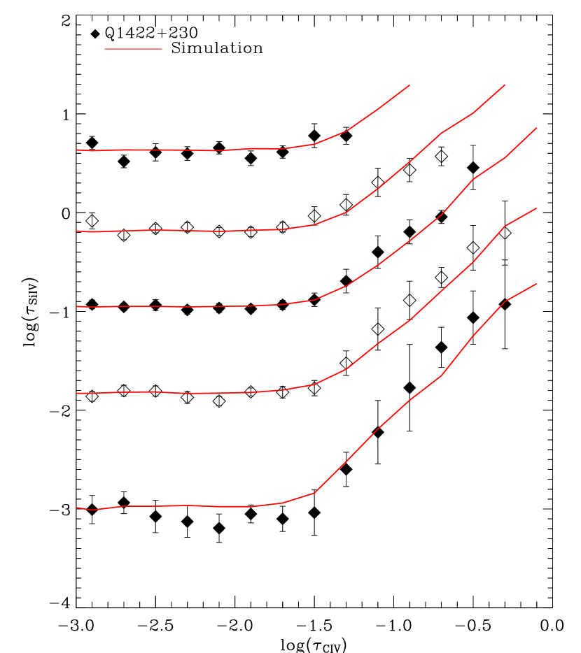
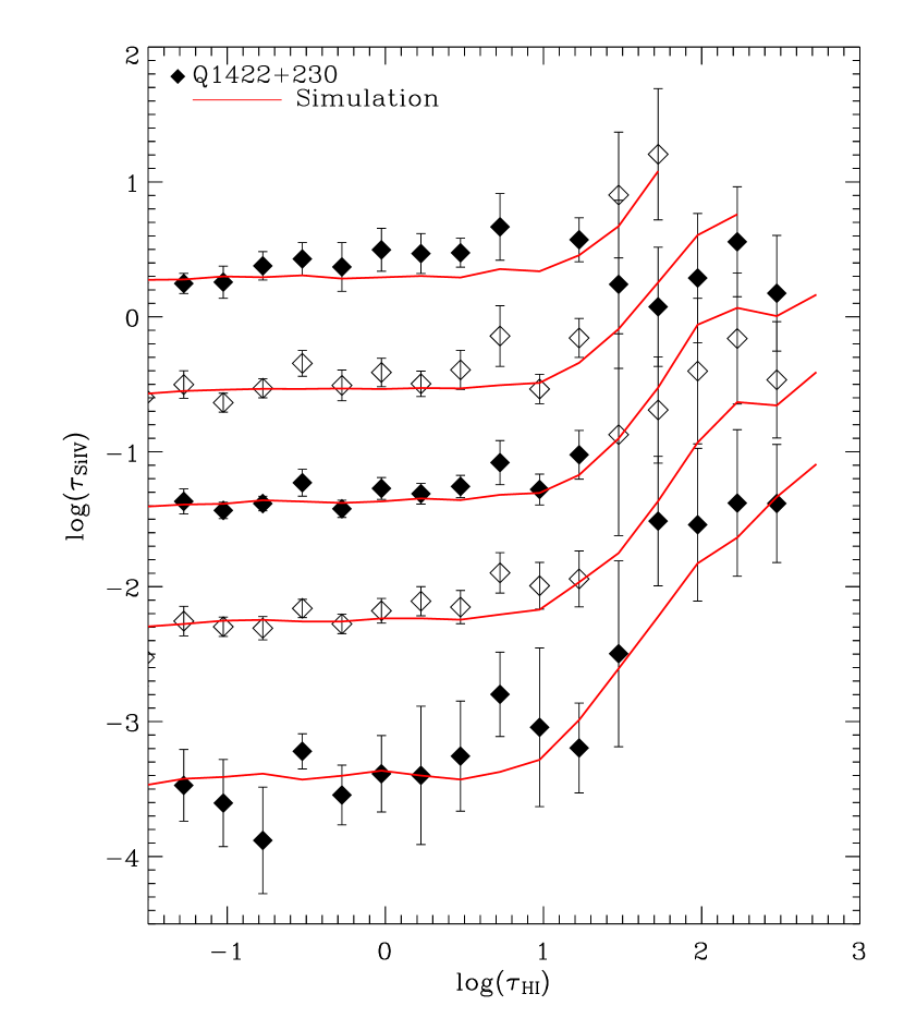
Figure 2.— SiIV optical depths in bins of $\tau_{\rm CIV}$ (left panel) and $\tau_{\rm HI}$ (right panel) for Q1422+230. From bottom to top, the points are the median, 69th, 84th, 93rd and 97th percentiles. Solid lines represent predictions from simulations with $\langle{\rm[C/H]}\rangle=-3.8+0.65\delta$, $\sigma=0.70$, and [Si/C]$=\log 5.$ For clarity, both observed points and simulated lines are plotted with vertical offsets of (from bottom to top) 0.0, 0.5, 1.0, 1.5, and 2.0 dex. Note that for the right panel the spectra have been smoothed by $7.5\,{\rm\,km\,s^{-1}}$ (see § 4.3).

For each observed quasar we generate 50 corresponding simulated spectra with the same noise properties, wavelength coverage, pixelization, instrumental broadening, and excluded regions. We apply to the simulated spectra the same automated continuum fitting routine as was used for the observations (Paper II, § 5.1, step 1; see also Paper I, § 4.1) to reduce any differences in the continuum fitting errors between simulated and observed spectra.

Before generating the spectra, we first impose a carbon distribution in the simulation that is consistent with the measurements presented in Paper II. In that paper we found that for a given overdensity and redshift, the probability distribution for the carbon abundance is well-described by a lognormal function, and we presented fits of the parameters of the distribution (i.e., the median and the width) as a function of overdensity and redshift for four different UVBs (Paper II, Eqn. 8 and Table 2). For the QG and Q ionizing backgrounds these fits are consistent with no evolution and we use the values for $z=3$; for models QGS and QGS3.2 we use, for each quasar, the median redshift of the analyzed region. We divide each simulation snapshot into $10^{3}$ cubes, and assign the gas particles in each section a carbon abundance of

$$[{\rm C}/{\rm H}]=\alpha+\beta(z-3)+\gamma(\log\delta-0.5)+s,$$

where $s$, which is the same for all particles in the sub-volume, is drawn at random from a lognormal distribution with mean 0 and variance $\sigma([{\rm C}/{\rm H}])=0.70$, and $\delta$ is the overdensity of the particle. For QG, $\alpha=-3.47$, $\gamma=0.65$, and $\beta=0$; for Q, $\alpha=-2.91$, $\gamma=0.17$, and $\beta=0$ (see Paper II, Table 2 for values used for other UVBs). Silicon abundances are assigned by assuming a constant value of [Si/C]. (The assumption that silicon tracks carbon perfectly is tested below.)

For each observed and simulated quasar spectrum, optical depths for pixels corresponding to absorption by H I, C IV, Si IV and Si III are extracted as described in §3.2. We may then plot various percentiles (such as the median) of the $\tau_{\rm SiIV}$ distribution for each bin in $\tau_{\rm CIV}$. The same procedure can be applied to correlate Si IV with H I, or Si III with Si IV. For each C IV (or other) bin, errors on the observed points are calculated by bootstrap resampling the spectrum, i.e., we divide the Ly$\alpha$ forest region of the spectrum into chunks of 5 Å which are bootstrap resampled to form a new realization of the spectrum (see Paper II §5.1, step 3). We require that in each bin there be at least five pixels above the percentile being computed, and that at least 25 pixels and five chunks contribute to the bin so that the errors are reliable; otherwise the point is discarded. For the simulations we compute 50 synthetic spectra and each percentile in each bin is set equal to the median of the 50 realizations, with errors given by bootstrap resampling the 50 simulated spectra. We require each bin of each realization to have at least five pixels above the given percentile, and to have at least five pixels and one chunk contributing to the bin, and we discard medians computed with fewer than five acceptable realizations.

For each percentile, the correlation disappears below some C IV optical depth $\tau_{c}$ at a value $\tau_{\rm min}$ that is determined by noise, continuum fitting errors, and contamination by other lines. These may be corrected for by subtracting $\tau_{\rm min}$ from the binned optical depths, thus converting points at $\tau_{\rm HI}<\tau_{c}$ into upper limits (Paper II, section 5.1, step 4, and Fig. 4). For each realization, we compute $\tau_{\rm min}$ as the given percentile of the optical depth for pixels with $\tau_{\rm HI}<\tau_{c}$, where $\tau_{c}=0.01$ is chosen as the C IV or Si IV optical depth below which we never see a correlation. The error on $\tau_{\rm min}$ for each realization is computed by bootstrap-resampling the quasar spectrum. When the realizations are combined, the value of $\tau_{\rm min}$ is computed as the median among the realizations, and the error on this value is computed by bootstrap-resampling the realizations.

The binned optical depth percentiles are then compared directly to the simulations, point by point. Because of slight differences in contamination, accuracy of continuum fitting, and noise, $\tau_{\rm min}$ for a given QSO may differ slightly from that of the simulations. Because we do not want to compare noise with noise, we either: A) subtract $\tau_{\rm min}$ from both simulations and observations before comparing, or B) add a constant to the simulated optical depths, chosen to minimize the difference between the simulations and observations for $\tau_{\rm HI}<\tau_{c}$; in this case we compare only points at $\tau_{\rm HI}\geq\tau_{c}$

4. Results

Before presenting the results from our full sample, we illustrate the optical depth statistics by showing some results from our QSO with the strongest signal, Q1422+230.

4.1. Results for Q1422+230

Fig. 2 shows several percentiles of $\tau_{\rm SiIV}$, binned according to their corresponding optical depth in C IV (left) and H I (right) for Q1422+230. The bottom points are medians, and the next four sets (with vertical offsets of 0.5,1.0, 1.5, and 2.0 dex) represent percentiles 69.146, 84.134, 93.319, and 97.725. These correspond to x=0, 0.5,1,1.5 and 2$\sigma$ values of the cumulative gaussian probability function $f(x)={1\over\sqrt{2\pi}}\int_{-\infty}^{x}e^{-t^{2}/2\sigma^{2}}dt$ (so that, for example, a distribution of $\tau_{\rm SiIV}$ that is lognormal with width $1\,$dex would give $1\,$ dex higher metallicity in the 84.134th percentile than in the median). The solid lines are predictions from the simulations with [Si/C]$=\log 5=0.70$ uniformly, median C metallicity $\langle{\rm[C/H]}\rangle=-3.8+0.65\delta$ and a width of $\sigma([{\rm C/H}])=0.70$ dex in the (lognormal) metallicity distribution.

The left panel shows that the simulations with the QG UVB and [Si/C]$=\log 5$ match the observations very well. This can be quantified by computing, for all points with $\log\tau_{\rm CIV}\geq\log\tau_{c}=-2.0$, the $\chi^{2}$ difference between the simulated and observed data points. We obtain $\chi^{2}/{\rm d.o.f.}=5.5/9,4.0/9,2.2/8,$ and 7.4/7 for the median, 0.5$\sigma$, 1$\sigma$ and 1.5$\sigma$ percentiles, respectively. The good fit of the median indicates that a uniform [Si/C] $\sim\log 5$ model fits well (though slightly higher [Si/C] are favored; see below), and that the data do not require any strong trend of [Si/C] with density (for which $\tau_{\rm CIV}$ is a proxy). Comparison of the higher percentiles can help constrain scatter in $\tau_{\rm SiIV}/\tau_{\rm CIV}$, which depends on the scatter in both [Si/C] and the ionization correction, and it is clear that that simulations with uniform [Si/C] and a uniform UVB fit the observations well; this is quantified below using our full data sample.

Comparison between simulated and observed $\tau_{\rm SiIV}$ versus $\tau_{\rm HI}$ (right) is somewhat less straightforward, as it depends both on [Si/C] and on the assumed distribution of carbon. Encouragingly, we find that for Q1422+230 a model with uniform [Si/C] (and carbon distribution as derived in Paper II from the full sample) fits the observed medians fairly well. The predicted higher percentiles are, however, a bit low; this is partly because the Q1422+230 C IV absorbers happen to exhibit slightly more metallicity scatter ($\approx 0.81\,$dex; see Paper II, § 5.2) than the level derived from the full sample.

In summary, the observed Q1422+230 Si IV optical depths, and their comparison to simulations show that: 1. A uniform [Si/C]$\sim\log 5$ is favored, 2. There is no evidence for a trend of [Si/C] with density, 3. There is no evidence for scatter in $\tau_{\rm SiIV}/\tau_{\rm CIV}$ beyond that included in the simulation with uniform [Si/C] and a uniform UVB.

4.2. $\tau_{\rm SiIV}$ versus $\tau_{\rm CIV}$ for the full sample

Figure 3.— Predicted optical depth ratios $\log\tau_{\rm SiIV}/\tau_{\rm CIV}$ as a function of the temperature and the hydrogen number density, assuming a solar ratio of Si/C. Solid (dashed) contours are for the UV-background model QG (Q) at $z=3$. The hatched region indicates the temperature range containing 90% of the particles at the given density.

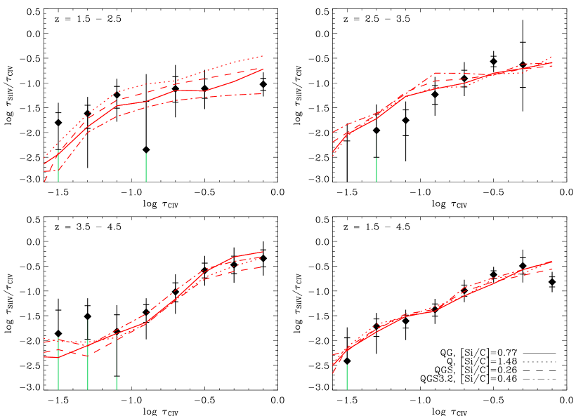
Figure 4.— Rebinned median $\log(\tau_{\rm SiIV}/\tau_{\rm CIV})$ vs. $\log\tau_{\rm CIV}$ in cuts of $z$ for the combined QSO sample. The first three panels show bins centered at $z=2.0,3.0$ and 4.0 with width $\Delta z=1.$; the bottom-right panel shows combined data from all redshifts. Lines represent corresponding rebinned simulation points (with errors suppressed, and with [Si/C] chosen to minimize the $\chi^{2}$) using different UVB models.

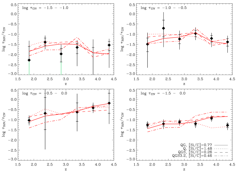
Figure 5.— Rebinned median $\log(\tau_{\rm SiIV}/\tau_{\rm CIV})$ vs. $z$ in cuts of $\tau_{\rm CIV}$ for the combined QSO sample. The first three panels show bins centered at $\log\tau_{\rm CIV}=-1.25,-0.75$ and -0.25 with width $0.5$ dex; the bottom-right panel shows data for all $\tau_{\rm CIV}$ combined. Lines represent corresponding rebinned simulation points (with errors suppressed, and with [Si/C] chosen to minimize the $\chi^{2}$) using different UVB models.

Table 1Recovered SiIV optical depths

QSO	$\log\tau_{{\rm CIV}}$	$\log\tau_{{\rm SiIV}},-0.5\sigma$		$\log\tau_{\rm SiIV},{\rm median}$		$\log\tau_{\rm SiIV},+0.5\sigma$		$\log\tau_{\rm SiIV},+1\sigma$		$\log\tau_{\rm SiIV},+1.5\sigma$		$\log\tau_{\rm SiIV},+2\sigma$
Q1422+230	-9.000	$\cdots$	$\cdots$	-3.047	0.088	-2.343	0.035	-1.959	0.031	-1.675	0.035	-1.354	0.047
Q1422+230	-3.900	-3.371	0.579	-2.530	0.153	-2.115	0.085	-1.898	0.071	$\cdots$	$\cdots$	$\cdots$	$\cdots$
Q1422+230	-3.700	$\cdots$	$\cdots$	-2.827	0.197	-2.183	0.092	-1.817	0.111	-1.622	0.105	$\cdots$	$\cdots$
Q1422+230	-3.500	$\cdots$	$\cdots$	-2.847	0.199	-2.308	0.076	-1.978	0.074	-1.765	0.049	$\cdots$	$\cdots$
Q1422+230	-3.300	$\cdots$	$\cdots$	-3.214	0.146	-2.492	0.114	-2.054	0.071	-1.786	0.127	-1.310	0.141
Q1422+230	-3.100	$\cdots$	$\cdots$	-2.879	0.139	-2.270	0.066	-1.918	0.058	-1.605	0.070	-1.326	0.072
Q1422+230	-2.900	$\cdots$	$\cdots$	-3.007	0.143	-2.361	0.049	-1.929	0.044	-1.583	0.082	-1.293	0.065
Q1422+230	-2.700	$\cdots$	$\cdots$	-2.936	0.110	-2.303	0.056	-1.954	0.039	-1.729	0.046	-1.482	0.064
Q1422+230	-2.500	$\cdots$	$\cdots$	-3.076	0.164	-2.306	0.052	-1.936	0.055	-1.661	0.044	-1.390	0.088
Q1422+230	-2.300	$\cdots$	$\cdots$	-3.127	0.160	-2.371	0.059	-1.985	0.043	-1.648	0.048	-1.402	0.069
Q1422+230	-2.100	$\cdots$	$\cdots$	-3.194	0.144	-2.409	0.047	-1.966	0.045	-1.691	0.041	-1.344	0.062
Q1422+230	-1.900	$\cdots$	$\cdots$	-3.050	0.090	-2.315	0.040	-1.974	0.039	-1.697	0.048	-1.450	0.075
Q1422+230	-1.700	$\cdots$	$\cdots$	-3.100	0.128	-2.318	0.059	-1.933	0.047	-1.647	0.050	-1.386	0.063
Q1422+230	-1.500	$\cdots$	$\cdots$	-3.037	0.230	-2.277	0.077	-1.882	0.068	-1.533	0.094	-1.221	0.121
Q1422+230	-1.300	$\cdots$	$\cdots$	-2.599	0.173	-2.024	0.125	-1.693	0.120	-1.421	0.104	-1.222	0.086
Q1422+230	-1.100	-3.610	0.606	-2.223	0.321	-1.678	0.213	-1.400	0.165	-1.194	0.143	$\cdots$	$\cdots$
Q1422+230	-0.900	-3.351	0.772	-1.773	0.439	-1.388	0.193	-1.195	0.121	-1.069	0.118	$\cdots$	$\cdots$
Q1422+230	-0.700	-1.873	0.313	-1.364	0.203	-1.156	0.102	-1.044	0.067	-0.930	0.095	$\cdots$	$\cdots$
Q1422+230	-0.500	-1.315	0.497	-1.063	0.270	-0.856	0.226	-0.545	0.225	$\cdots$	$\cdots$	$\cdots$	$\cdots$
Q1422+230	-0.300	-1.264	0.813	-0.928	0.450	-0.706	0.325	$\cdots$	$\cdots$	$\cdots$	$\cdots$	$\cdots$	$\cdots$
Q1422+230	-0.100	$\cdots$	$\cdots$	$\cdots$	$\cdots$	$\cdots$	$\cdots$	$\cdots$	$\cdots$	$\cdots$	$\cdots$	$\cdots$	$\cdots$

Note. — Columns 1 and 2 contain the quasar name and the recovered CIV optical depth respectively. Columns 3 and 4 contain the 31st percentile of the recovered SiIV optical depth and the $1\sigma$ error on this value. The remaining columns show the same quantities for higher percentiles (50th, 69th, 84th, 93th, and 98th). A CIV optical depth of $\log\tau_{\rm CIV}=-9$ indicates that the corresponding $\tau_{\rm SiIV}$ are the $\tau_{\rm min}$ values. The complete version of this table, including all quasars, is in the electronic edition of the Journal. The printed edition contains only data for Q1422+230.

To place more quantitative constraints on [Si/C], test for evolution, and make a more detailed comparison with several UVB models, we have combined the data points obtained from our entire sample.(These points are tabulated in Table 1.) Figure 4 shows $\log\tau_{\rm SiIV}/\tau_{\rm CIV}$ versus $\log\tau_{\rm CIV}$, in bins of $z$. To generate these points, we begin with $\tau_{\rm SiIV}$ values binned in $\tau_{\rm CIV}$, as in Fig. 2. We then subtract from each the “flat level” $\tau_{\rm min}$ for that QSO to adjust for noise, contamination etc. (see § 3), then divide by the central value of the $\tau_{\rm CIV}$ bin. These points, gathered from all QSOs, are rebinned by $\chi^{2}$-fitting, for each $\tau_{\rm CIV}$ range indicated in Fig. 4, a constant level to all of the points in the specified redshift range. The errors represent 1- and 2-$\sigma$ confidence intervals ($\Delta\chi^{2}=2$ and $\Delta\chi^{2}=4$).

The plotted lines indicate predictions from the simulations for our different UVBs; our fiducial model, QG, is shown in solid lines. For each background, we generate simulated $\tau_{\rm SiIV}/\tau_{\rm CIV}$ points in the same way as we did for the observations, but averaging over 50 simulated realizations as described in § 3.4. We then calculate a $\chi^{2}$ between all valid observed original (not rebinned) points and the corresponding simulated points. Because we use 50 simulated realizations, the simulation errors are almost always negligible compared to the observed errors, but they are still taken into account by calculating the total $\chi^{2}$ using the formula:

$$\chi^{2}=\sum_{i}\left[\left({X_{\rm obs}-X_{\rm sim}\over\sigma_{\rm obs}}\right)^{-2}+\left({X_{\rm obs}-X_{\rm sim}\over\sigma_{\rm sim}}\right)^{-2}\right]^{-1},$$ (1)

where $X\equiv\tau_{\rm SiIV}/\tau_{\rm CIV}$ and $\sigma$ is the error in this quantity. We then add a constant offset to the simulated points (which corresponds to scaling [Si/C]) such that $\chi^{2}$ is minimized. In each panel the lines connect the scaled, rebinned simulation points.

The first clear result is that there is a strong trend of $\log(\tau_{\rm SiIV}/\tau_{\rm CIV})$ with $\log\tau_{\rm CIV}$, from $\lesssim-2$ at $\log\tau_{\rm CIV}\sim-1.5$ to $\gtrsim-1.0$ at $\log\tau_{\rm CIV}\gtrsim-0.5$. This previously unnoted correlation is expected if [Si/C] is constant and $\tau_{\rm CIV}$ correlates with density, since (as shown in Fig. 3) $\tau_{\rm SiIV}/\tau_{\rm CIV}$ increases rapidly with gas density. As shown by the simulation lines, this trend is reproduced in all redshift bins by the simulations for all of our UVB models. Comparing the first three panels shows that while $\tau_{\rm SiIV}/\tau_{\rm CIV}$ correlates strongly with $\tau_{\rm CIV}$, there is little dependence on redshift. This can be seen more clearly in the first three panels of Fig. 5, which show $\log(\tau_{\rm SiIV}/\tau_{\rm CIV})$ versus $z$ in bins of $\tau_{\rm CIV}$. There is no evidence, in either the simulated or the observed points, for evolution in $\tau_{\rm SiIV}/\tau_{\rm CIV}$, except perhaps for a slight increase in $\tau_{\rm SiIV}/\tau_{\rm CIV}$ with increasing $z$ at the highest densities.

Table 2Best fit [Si/C] and $\chi^{2}/{\rm d.o.f.}$

UVB model	best fit [Si/C]	$\chi^{2}$/d.o.f.
QG	$0.77^{+0.05}_{-0.05}$	65.7/115
Q	$1.48^{+0.05}_{-0.06}$	65.6/115
QGS	$0.26^{+0.06}_{-0.07}$	73.8/115
QGS3.2	$0.46^{+0.10}_{-0.08}$	85.2/115

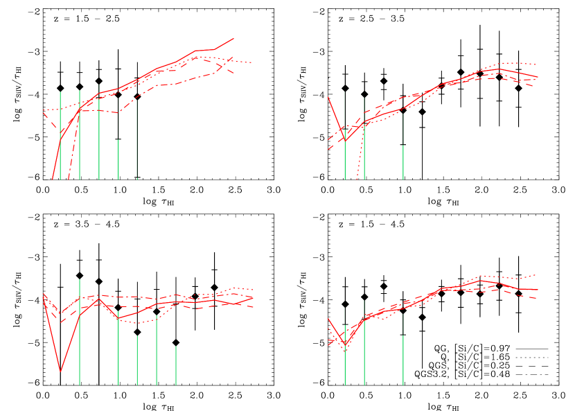
Figure 6.— Median $\log(\tau_{\rm SiIV}/\tau_{\rm HI})$ vs. $\log\tau_{\rm HI}$ in bins of $z$ for the combined QSO sample. The first three panels show bins centered at $z=2,3,$ and 4 with width $\Delta z=1$; the bottom-right panel shows combined data for all redshifts. The lines represent corresponding simulation points (with errors suppressed) using different UVB models.

The observed trends in $\log(\tau_{\rm SiIV}/\tau_{\rm CIV})$ are reproduced well by the simulations. Because $\tau_{\rm SiIV}/\tau_{\rm CIV}$ scales with Si/C, the offset in $\tau_{\rm SiIV}/\tau_{\rm CIV}$ obtained by minimizing the $\chi^{2}$ (Eq. 1) against the observations can be used to compute the best fit [Si/C]. For our fiducial UVB model QG, the simulated spectra were generated with [Si/C]=0.70, we find an offset of $+0.07$ dex (implying a best-fit [Si/C]=0.77) with $\chi^{2}/{\rm d.o.f.}$=65.7/115. As we found in Paper II and for Q1422+230 above, the reduced $\chi^{2}$ is somewhat low; in Paper II we showed that his was largely due to a slight overestimate of the errors at low-$\tau_{\rm CIV}$.

The fitted [Si/C] values and corresponding $\chi^{2}/{\rm d.o.f.}$, are listed in Table 2, with errors computed by bootstrap-resampling the quasars used in the $\chi^{2}$ minimization. For our fiducial model, QG, the best fit [Si/C]$=0.77^{+0.05}_{-0.05}$. The quasar-only background Q (which is probably too hard; see Paper II) gives a higher values of [Si/C]$=1.48^{+0.05}_{-0.06}$, and the softer QGS and QGS3.2 backgrounds give lower values than QG by $\approx 0.3-0.5$ dex. Note that the QGS background is unrealistically soft at $z\;\hbox to0.0pt{\lower 2.5pt\hbox{$\sim$}\hss}\raise 1.5pt\hbox{$<$}\;3$ (see Paper II), but the QGS3.2 background may be plausible.

Because the $\tau_{\rm SiIV}/\tau_{\rm CIV}$ ratio depends on both [Si/C] and the shape of the UVB, its measurement can be used to study the evolution of the UVB under the assumption that [Si/C] is constant. Songaila (1998, see also Songaila & Cowie 1996) has measured the median Si IV/C IV ratio versus $z$ for C IV systems of column density $5\times 10^{12}\,{\rm cm^{-2}}\leq N({\rm CIV})\leq 10^{14}\,{\rm cm^{-2}}$ and found evidence for strong evolution, as well as a sharp break in $\tau_{\rm SiIV}/\tau_{\rm CIV}$ at $z=3.0.$ This was interpreted as evidence for a sudden softening of the UVB at $z>3$. However, in a recent study Boksenberg et al. (2003), in agreement with their earlier work and that of Kim, Cristiani, & D’Odorico (2002) find no evolution in $\tau_{\rm SiIV}/\tau_{\rm CIV}$ in their sample of $10^{12}\,{\rm cm^{-2}}\leq N({\rm CIV})\lesssim 3\times 10^{14}\,{\rm cm^{-2}}$ absorbers. As discussed above (see Fig. 5), we see no evidence for evolution in the median $\tau_{\rm SiIV}/\tau_{\rm CIV}$ stronger than that predicted by the simulations, in any of our $\tau_{\rm CIV}$ bins, or when all $\tau_{\rm CIV}$ values are combined (Fig. 5, bottom-right).

Because $\tau_{\rm SiIV}/\tau_{\rm CIV}$ varies by $\sim 1.5\,$dex in correlation with $\tau_{\rm CIV}$, its evolution is best assessed by using only a small window in $\tau_{\rm CIV}$; otherwise evolution in the weight provided by each $\tau_{\rm CIV}$ – whether due to selection effects or evolution in the distribution of $\tau_{\rm CIV}$ – may lead to apparent evolution in $\tau_{\rm SiIV}/\tau_{\rm CIV}$. In our analysis, in which we use small cuts in $\tau_{\rm CIV}$, we see no evidence for evolution in the UVB beyond that in the smoothly changing QG and Q models; indeed, the QGS3.2 model with an artificial change in softness at $z=3.2$ is disfavored by our data, having a significantly higher $\chi^{2}$ than either the QG or Q models.

The simulations we employ assume a constant and uniform [Si/C]; but because the formation mechanism for Si and C may be different this need not be the case. We can, however, observationally constrain the scatter in [Si/C] by repeating our determination of it using different percentiles in $\tau_{\rm SiIV}/\tau_{\rm CIV}$. If the probability distribution of [Si/C] for fixed $\tau_{\rm CIV}$ is, like that of [C/H] and [Si/H] for fixed $\tau_{\rm HI}$, lognormal, then we can directly constrain the width $\sigma({\rm[Si/C]})$ of the distribution by comparing [Si/C] derived for different percentiles. For the 69th, 84th, 93rd and 97th percentiles, we obtain [Si/C]=$0.73^{+0.05}_{-0.06}$, $0.64^{+0.07}_{-0.07}$, $0.58^{+0.13}_{-0.04}$, and $0.78^{+0.10}_{-0.14}$, respectively. This translates into a rough 2$\sigma$ upper limit of $\sigma({\rm[Si/C]})\lesssim 0.04\,$dex. As a rough test of this upper limit, we have generated simulated spectra with a median ${\rm[Si/C]=0.77}$ and the usual C distribution, but with a lognormal scatter in [Si/C] of width $\sigma({\rm[Si/C]})$. If we add the $\chi^{2}$ for the 69th, 84th and 93rd percentiles for quasars at $z\geq 3$ (there is little useful information on the upper percentiles from $z<3$), we find $\chi^{2}/{\rm d.o.f.}=198.0/185$ for no scatter in [Si/C], and $\chi^{2}=198.2,203.4,$ and 223.0 for $\sigma({\rm[Si/C]})=0.1,0.2,$and 0.4 dex, respectively. Because the percentiles are correlated these cannot be correctly translated directly into confidence limits; however they suggest that the data are compatible with $\sigma({\rm[Si/C]})=0.1$, but probably not with $\sigma({\rm[Si/C]})=0.2$ and almost certainly not with $\sigma({\rm[Si/C]})=0.4$. Thus, contrary to the large scatter in [C/H], $\sigma({\rm[C/H]})\approx 0.7$ dex found in Paper II, there appears to be very little scatter in [Si/C].

We may also subdivide our sample by redshift and density to test the dependence of [Si/C] on these. First, computing [Si/C] using only spectra that have a median absorption redshift ${\rm med}(z)>3.0$ (see Paper II, Table 1) yields [Si/C]=$0.76^{+0.05}_{-0.07}$, versus [Si/C]=$0.79^{+0.10}_{-0.08}$ using the spectra with ${\rm med}(z)<3.0$. The [Si/C] values inferred from the redshift subsamples are also (marginally) consistent for the Q and QGS UVBs, but inconsistent for QGS3.2; the latter would imply a jump from [Si/C]$=0.77^{+0.05}_{-0.09}$ at $z>3$ to [Si/C]$=0.32^{+0.08}_{-0.13}$ at $z<3$. This is a second way of seeing that our data disfavors a sudden change in UVB hardness near $z=3$, assuming that [Si/C] is constant.

To test for variation in [Si/C] with overdensity $\delta$ we have recomputed [Si/C] using only pixels with $\tau_{\rm HI}$ corresponding to $\delta<20$ or $\delta>20$ (using the $\tau_{\rm HI}$-$\delta$ conversion of Paper II, Fig. 2). We obtain [Si/C]=$0.87^{+0.19}_{-0.10}$ for the low-density sample, versus [Si/C]=$0.73^{+0.03}_{-0.05}$ at high density. This difference could imply either that [Si/C] is higher at low densities, or that the UVB is softer than we have assumed (see Fig. 3); but the effect is only significant at the $\approx 1.3\sigma$ level.

4.3. $\tau_{\rm SiIV}$ versus $\tau_{\rm HI}$ for the full sample

While the $\tau_{\rm SiIV}/\tau_{\rm CIV}$ ratios give the most direct constraints on [Si/C], it is also useful to examine $\tau_{\rm SiIV}/\tau_{\rm HI}$: comparing the simulated to the observed $\tau_{\rm SiIV}/\tau_{\rm HI}$ ratios gives, in principle, a second estimate of [Si/C]. This inference, however, is less reliable than that from $\tau_{\rm SiIV}/\tau_{\rm CIV}$ for two reasons. First, it includes the uncertainty in [C/H], which is largest at the relatively high densities at which (because of the small Si IV/Si fraction at lower densities) Si IV is best-detected. Second, Si absorption lines have a much smaller thermal width than hydrogen lines, and are only observable in relatively high-density gas (where Hubble broadening is small). This leads to significant differences between the Si IV-weighted and H I-weighted densities (see Paper II, § 4.3, Paper I, § 5.3), i.e., the Si IV and H I absorption do note arise from exactly the same gas. The effect of this is to skew (and weaken) the correlation of $\tau_{\rm SiIV}$ with $\tau_{\rm HI}$ in a way that depends on the H I column-density distribution. Unfortunately, as discussed by Theuns et al. (2002), the simulation does not exactly reproduce the observed $N({\rm HI})$ distribution at the high-column density end (which is most important for the present study), so the “skewing” may be somewhat different in observed and simulated correlations, and render conclusions about [Si/H] unreliable.

The problems arising from differential line broadening can be partially remedied by smoothing the spectra so that the minimal line widths of all species become similar; experimentation shows that smoothing the spectra by convolving them with a Gaussian with FWHM of $\approx 5-10\,{\rm\,km\,s^{-1}}$ significantly increases the strength of the signal, and a smoothing of 7.5 ${\rm\,km\,s^{-1}}$ has been adopted for the calculations shown in Figs. 2 and 6. Fig. 6 shows $\log\tau_{\rm SiIV}/\tau_{\rm HI}$ versus $\log\tau_{\rm HI}$ in bins of $z$ for our combined sample. Lines again connect the corresponding simulation points (with an overall scaling to best match the observations) that reproduce the observed trends in $z$ and $\tau_{\rm HI}$. The scalings correspond to best-fit [Si/C] values of $0.97\pm 0.08$, $1.65\pm 0.08$, $0.25\pm 0.07$ and $0.48\pm 0.09$ for QG, Q, QGS, and QGS3.2 respectively, slightly higher than the values found above using $\tau_{\rm SiIV}/\tau_{\rm CIV}$. However, as explained above, these values depend on the degree of smoothing: for example, with no smoothing, we recover values $\approx 0.1-0.3\,$dex higher yet. Since it is unclear which smoothing level gives the correct results, the inferences of [Si/C] using $\tau_{\rm SiIV}/\tau_{\rm HI}$ should not be relied on.

The same difference in thermal width affects inferences using Si IV/C IV, but at a lower level; whether or not we smooth by 7.5${\rm\,km\,s^{-1}}$ changes the inferred [Si/C] by $\sim 0.1$ dex, which is a reasonable estimate of the induced systematic error.

Figure 7.— Predicted optical depth ratios $\log\tau_{\rm SiIII}/\tau_{\rm SiIV}$ as a function of the temperature and the hydrogen number density. Solid (dashed) contours are for the UV-background model QG (Q) at $z=3$. The hatched region indicates the temperature range containing 90% of the particles at the given density.

4.4. $\tau_{\rm SiIII}$ versus $\tau_{\rm SiIV}$ for the full sample

A final correlation that we have examined is that of $\tau_{\rm SiIII}/\tau_{\rm SiIV}$ with $\tau_{\rm SiIV}$. Fig. 7 shows the predicted $\tau_{\rm SiIII}/\tau_{\rm SiIV}$ versus the temperature $T$ and density $n_{\rm H}$ of the absorbing gas. For high $T$, $\tau_{\rm SiIII}/\tau_{\rm SiIV}$ becomes independent of $n_{\rm H}$, and declines rapidly with $T$. Thus, the presence of Si III can be used to constrain the temperature of the gas providing Si IV absorption. In Paper II a similar test was carried out using the $\tau_{\rm CIII}/\tau_{\rm CIV}$ ratio, yielding the constraint $T<10^{5.0}\,$K.

Fig. 8 shows $\tau_{\rm SiIII}/\tau_{\rm SiIV}$ versus $\tau_{\rm SiIV}$ for our full sample, for three cuts in $z$. At $\log\tau_{\rm SiIV}\gtrsim-1.2$ and $2.5\leq z\leq 3.0$ (where the data are particularly good) $-0.5\lesssim\tau_{\rm SiIII}/\tau_{\rm SiIV}\lesssim 0.5$, corresponding to a direct upper limit of $T\lesssim 10^{4.9}-10^{5.1}\,$K for the bulk of the gas giving rise to this Si IV absorption (the lower value pertaining to the higher end of the $\tau_{\rm SiIV}$ range.) The simulations give predictions that depend only very weakly on the UVB model and are in good agreement with the data, particularly at $2.5\leq z\leq 3.0$ (however note that at $z\gtrsim 3.0$ there is somewhat more Si III absorption predicted than observed for high $\tau_{\rm SiIV}$). Concentrating on the QG model, we find $\chi^{2}/{\rm d.o.f.}=80.5/114$ comparing all simulated and observed points with $\log\tau_{\rm SiIV}\geq-2.0$. Fitting an offset to the median $\log\tau_{\rm SiIII}/\tau_{\rm SiIV}$ ratios (as done above for $\tau_{\rm CIV}/\tau_{\rm SiIV}$) we find $-0.32_{-0.16}^{+0.14}\,$dex, indicating that simulations predict somewhat too much Si III absorption overall. We have repeated this exercise for the 16th, 31st, 69th and 84th percentiles in order to fit the center and width $\sigma({\rm[SiIII/SiIV]})$ of a lognormal distribution governing scatter in $\tau_{\rm SiIII}/\tau_{\rm SiIV}$ beyond that present in the simulations. The fit obtained indicates that overall the observed $\tau_{\rm SiIII}/\tau_{\rm SiIV}$ ratio is lower by $0.15\pm 0.06\,$dex than that for the simulations, with $\sigma({\rm[SiIII/SiIV]})=0.07\pm 0.07\,$dex. These results imply that most of the gas is cool enough to be consistent with the photoionization equilibrium assumed in the simulations, and that the scatter in $\tau_{\rm SiIII}/\tau_{\rm SiIV}$ is similar to that in the simulations. But they are also consistent with a (small) contribution by hotter gas to the observed Si IV optical depths.

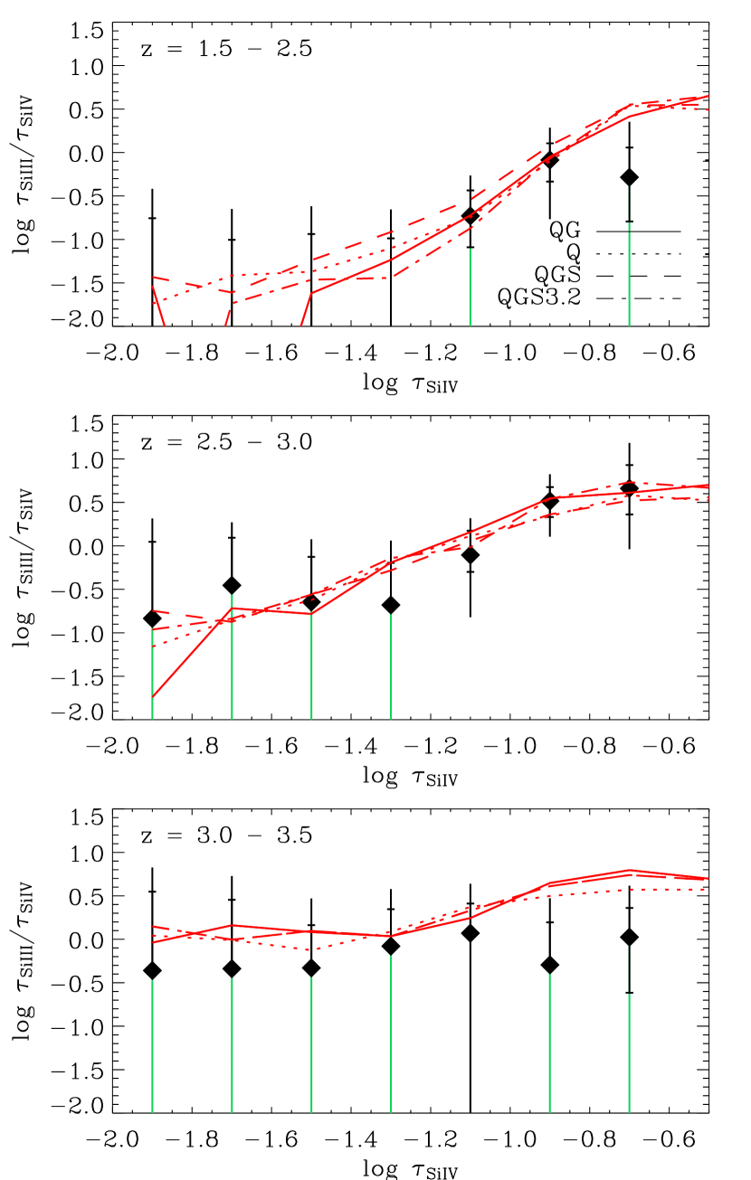
Figure 8.— Ratios of median $\tau_{\rm SiIII}/\tau_{\rm SiV}$ versus $\tau_{\rm SiIV}$ in bins of $z$ for the full sample. The lines represent corresponding simulation points (with errors suppressed) using different UVB models.

5. Analysis and discussion of results

We have shown that the pixel optical depth correlations derived from our observed QSO spectra are consistent, in detail, with spectra drawn from a hydrodynamical simulation with: 1) an assumed carbon metallicity distribution as derived in Paper II from measurements of C IV absorption, 2) a uniform (rescaled) UVB model taken from Haardt & Madau (2001), and 3) a constant and uniform [Si/C] value.

We have used this success to draw inferences regarding [Si/C] for each of several models of the UVB. Before analyzing these inferences it is worth discussing some effects that bear on their robustness.

5.1. Uncertainties

UVB spectral shape: Our inference of [Si/C] obviously depends on the assumed shape and evolution of the UVB: the models used here produce a range $0.26\leq{\rm[Si/C]}\leq 1.48$. These models, however, span a range of possibilities that is larger than that allowed by independent observations. The harder model Q, for example, was found in Paper II to produce a mean carbon abundance that increases with decreasing density, which is probably unphysical. Likewise the softer model QGS was found to imply increasing [C/H] with $z$, also unphysical. The model QGS3.2, with a sudden transition at $z=3.2$, produced no problems in Paper II, but here we find that the resulting predicted jump in $\tau_{\rm SiIV}/\tau_{\rm CIV}$ is disfavored by our observations. Our fiducial model QG appears compatible (and produces physical results) for all of our metallicity measurements thus far; it therefore seems unlikely that this UVB is very far in error. Note, however, that Boksenberg et al. (2003) found that they were unable to fit Si II/Si IV vs. C II/C IV column density ratios in their data (probing higher densities than our analysis) using Haardt & Madau (2001) models.

UVB inhomogeneity: We have assumed that the UVB is perfectly uniform, which is probably unrealistic. However, we can limit the non-uniformity of the hardness of the UVB because such non-uniformity would lead to scatter in $\tau_{\rm SiIV}/\tau_{\rm CIV}$ even for uniform [Si/C], whereas our measurement of the higher percentiles in $\tau_{\rm SiIV}/\tau_{\rm CIV}$ proved to be compatible with the predictions of the simulations for a uniform [Si/C].

Collisionally ionized gas: The simulation we have employed does not contain feedback from star formation and therefore contains only the hot ($T\gg 10^{5}\,$K) gas resulting from heating by accretion shocks. If the true universe has hot gas not present in our simulations, our inferences could be biased. We have put a constraint $T\lesssim 10^{4.9}\,$K on the temperature of the bulk of the gas giving rise to the Si IV absorption, using the $\tau_{\rm SiIII}/\tau_{\rm SiIV}$ ratio. The simulation, however, does predict slightly higher $\tau_{\rm SiIII}/\tau_{\rm SiIV}$ overall, by $\approx 0.3\,$dex using the median and by $\approx 0.15\,$dex using all percentiles. Although this might be attributed to some systematic difference between simulations and observations, it may indicate that some fraction ($\lesssim 30\%$, since that is the lowest percentile we probe) of the Si IV absorbing gas is hotter ($T>10^{5}\,$K) than in the simulations. Note also that, as in Paper II, we can put no constraint on metals in gas that is either too hot ($T\gg 10^{5}\,$K) or too cold ($T\ll 10^{4}$ K) to cause detectable Si IV or C IV absorption.

Uncertainties in recombination rates: Savin (2000) has pointed out that the Si IV and C IV dielectric recombination rates used in CLOUDY may be uncertain by up to $\sim 0.3$ dex, leading to uncertainties in inferred [Si/C]. Considering first C IV, the laboratory work of Schippers et al. (2001), with quoted uncertainties of $\sim 15\%$, finds rates $\sim 15-30\%$ higher than those used in CLOUDY version 94. The calculation of Savin (2000) suggest that if the CLOUDY rate were $30\%$ too low, we would overestimate [Si/C] by a factor that depends on the density of the absorbing gas and varies from $\sim 0.0-0.07$ dex for the range given below in § 5.2. For Si IV the situation is worse because there are no published laboratory experiments, so the rate could be uncertain by $\pm 0.3$ dex (Savin, 2000). If the CLOUDY rate were too high (resp. too low) by $0.3\,$dex, we would overestimate (resp. underestimate) [Si/C] by $0.2\,$dex at the highest gas densities we probe, by a negligible amount at the lowest densities, and probably by $\sim 0.1\,$dex overall.

Note also that differences in the Si and C line widths, as discussed in § 4.3 could lead to an uncertainty of $\sim 0.1\,$dex in inferred [Si/C] using our method.

5.2. Corresponding gas and column densities

We have analyzed Si IV, C IV, and H I pixel optical depths to draw inferences regarding the cosmic silicon abundance. For these to be compared with those from theoretical or observational studies, it is useful to estimate the gas densities and the H I and C IV line column densities our measurements pertain to.

In measuring $\tau_{\rm SiIV}/\tau_{\rm HI}$ vs. $\tau_{\rm HI}$, (Fig. 6), we obtain 2$\sigma$ detections for $0.75\lesssim\log\tau_{\rm HI}\lesssim 2.5$ for $2.5\leq z\leq 3.5$ (where our data are best). Using the theoretical $\tau_{\rm HI}$-density relation given in Paper II, this range corresponds at $z=3$ to $0.5\lesssim\log\delta\lesssim 2.0$. (Note, however, that the upper limit results from the inability to recover high-$\tau_{\rm HI}$ pixels and does not apply to results binned in $\tau_{\rm CIV}$.) These densities can be converted into approximate H I column densities using the theoretical relation $N_{\rm HI}\sim 10^{15}\,{\rm cm^{-2}}(\delta/10)^{3/2}[(1+z)/4]^{9/2}$ from Schaye (2001), to obtain a column density range

$$2\times 10^{14}\,{\rm cm^{-2}}\lesssim N_{\rm HI}\lesssim 3\times 10^{16}\,{\rm cm^{-2}}.$$ (2)

Another way to estimate the H I column densities corresponding to the H I optical depth range over which we detect Si IV is to use the relation between column density $N$ and optical depth $\tau_{c}$ at the center of a line of width $b$,

$$\tau_{c}=0.76\left({f\lambda_{0}\over f_{\rm HI}\lambda_{0,{\rm HI}}}\right)\left({N\over{10^{13}}\,{\rm cm^{-2}}}\right)\left({b\over 10\,{\rm km\,s^{-1}}}\right)^{-1},$$ (3)

where $f$ and $\lambda_{0}$ are the oscillator strength and the rest wavelength respectively. Using $b=25~{}{\rm km\,s^{-1}}$ yields $2~{}\times~{}10^{14}{\rm cm^{-2}}\lesssim N_{\rm HI}\lesssim 1\times 10^{16}{\rm cm^{-2}}$, in close agreement with our earlier estimate. We can estimate the C IV column density range in a similar way. From Fig. 4 we see that Si IV is detected over the range $-1.5\lesssim\log\tau_{\rm CIV}\lesssim 0.0$, which corresponds to

$$7\times 10^{11}{\rm cm^{-2}}\lesssim N_{\rm CIV}\lesssim 2\times 10^{13}{\rm cm^{-2}},$$ (4)

for a typical C IV line width of $10~{}{\rm km\,s^{-1}}$.

Note also that our analysis pertains to significantly lower physical densities than results obtained using the C II/C IV ratio as a density tracer (Songaila, 1998; Boksenberg et al., 2003); using Fig. 23 of Boksenberg et al. (2003), our upper density limit corresponds roughly to $N({\rm CII})/N({\rm CIV})\lesssim-1.5$.

5.3. Comparison to Nucleosynthetic yield studies

The small scatter in [Si/C] implies that silicon and carbon share a common enrichment mechanism, and both the high [Si/C] and early enrichment epoch we observe suggest enrichment by massive stars. It is therefore interesting to compare our [Si/C] to that predicted in theoretical supernova yields for low-metallicity, zero metallicity, and (more speculatively) supermassive progenitors. The yields of Woosley & Weaver (1995), integrated over a Salpeter initial mass function (IMF) with slope between -2.5 and -0.5, give production factors (yields relative to solar metallicity) of $0.4\lesssim{\rm[Si/C]}\lesssim 0.6$ for $10^{-4}\leq Z/Z_{\odot}\leq 0.1$ progenitor metallicities. At $Z=0$, significantly smaller [Si/C] results: Woosley & Weaver (1995) and Heger & Woosley (2002) give production factors [Si/C]$\simeq 0.15$ for massive 12-40${\rm\,M_{\odot}}$ stars, and [Si/C]$\sim 0.0-0.2$ for $15-30{\rm\,M_{\odot}}$ metal-free stars are also quoted by Chieffi & Limongi (2002) from both their own calculations and those of Umeda & Nomoto (2002). Zero metallicity also, however, allows (at least theoretically) for supermassive stars with quite different yields. Heger & Woosley (2002) provide yields of [Si/C]$\simeq 1.2$ for supermassive (140-260${\rm\,M_{\odot}}$) progenitors that produce pair-instability supernovae. Including as well the massive ($12-40{\rm\,M_{\odot}}$) stars with a Salpeter IMF gives [Si/C]$\simeq 0.85$.

We may also compare our [Si/C] values to those in metal-poor stars, but here there are a range of results, and substantial uncertainties – particularly with regard to C – concerning the importance of mixing and accretion from a companion (e.g., Carretta, Gratton, & Sneden, 2000). The lowest-metallicity (${\rm[Fe/H]}\lesssim-2.5$) halo stars give typically [Si/C]$\sim-0.4-+0.5$ (e.g., Chieffi & Limongi, 2002; Norris, Ryan, & Beers, 2001; Depagne et al., 2002; McWilliam et al., 1995). For $-2.5\leq{\rm[Fe/H]}\leq-1.5$, somewhat higher values are apparently seen: measurements of $-0.5\lesssim{\rm[C/Fe]}\lesssim 0.0$ and $0.2\lesssim{\rm[Si/Fe]}\lesssim 0.7$ (see the compilation by Norris et al. 2001) suggest ${\rm[Si/C]\sim 0.7}$, and McWilliam et al. (1995) finds values of ${\rm[Si/C]}\sim 0.2-1.2$. However, Carretta, Gratton, & Sneden (2000) find higher [C/Fe] of $-0.2\lesssim{\rm[C/Fe]}\lesssim 0.3$ when using only unmixed stars, implying somewhat smaller ${\rm[Si/C]}\sim 0.4$.

If we assume that our fiducial UVB model (and assumed recombination rates; see §5.1) are correct, then the inferred [Si/C]$=0.77\pm 0.05$ has interesting implications. It is substantially higher than the [Si/C] predicted from $\lesssim 40{\rm\,M_{\odot}}$ Population III stars with a standard IMF, and it is somewhat ($\sim 0.2\,$dex) higher than abundance ratios in low-metallicity stars, and predicted yields for massive Population II stars. If the latter discrepancy is taken seriously, it could be remedied by including some supermassive (pair-instability) supernovae as modeled by Heger & Woosley (2002).

If, instead, we assume that [Si/C] should be $\sim 0.5$ on the basis of standard nucleosynthesis yields, then we infer that the UVB must be softer (at bith low- and high-$z$) than our fiducial model QG. However, it should be noted that a UVB as soft as model QGS, for which we find [Si/C]$=0.26$, was demonstrated to produce unphysical results in Paper II.

5.4. Implications for cosmic abundances

In § 4 we measured [Si/C] values for several UVB models by comparing observations of $\tau_{\rm SiIV}/\tau_{\rm CIV}$ to simulations generated using a given UVB model and a distribution of [C/H] as determined in Paper II (§ 7) for that UVB. Combining these fits (See Table 2) with the results of Paper II enables us to assess the overall cosmic abundance of silicon. For these calculations we assume that our derived [Si/C] is uniform and constant, but we include the uncertainty in its determination.

In Paper II we combined the median [C/H]$(\delta,z)$ with the width $\sigma([{\rm C/H}])(\delta,z)$ of the lognormal probability distribution of [C/H] for $-0.5\leq\log\delta\leq 2.0$ to determine the mean C abundance versus $\delta$. This was then integrated over the mass-weighted probability distribution $\delta$ (obtained from our hydrodynamical simulation) to compute the contribution by gas in this density range to the overall mean cosmic [C/H]. Assuming that [Si/C] is constant over this density range we obtain, for our fiducial UVB model QG, [Si/H]$=-2.03\pm 0.14$, corresponding to

$$\Omega_{\rm Si,IGM}\simeq 3.4\times 10^{-7}10^{[{\rm Si}/{\rm H}]+2.0}\left({\Omega_{b}\over 0.045}\right),$$ (5)

with no evidence for evolution. Extrapolating our [C/H] and [Si/C] results to the full density range of the simulation would yield values $\approx 0.2$ dex higher. For a harder UVB, the inferred cosmic Si abundance would be significantly higher, as both the inferred [C/H] and [Si/C] increase with the UVB hardness. For our quasar-only model Q, we obtain a contribution of [Si/H]$\approx-0.8$, or $\Omega_{\rm Si}\approx 5\times 10^{-6}$. For comparison, Songaila (2001) found, using a direct sum of Si IV lines, that $\Omega_{\rm SiIV}=(0.5-2)\times 10^{-8}$. This indicates that although Songaila’s results provide a useful lower limit, an ionization correction of more than 10 (or even much larger for harder backgrounds) must be made to translate $\Omega_{\rm SiIV}$ into an estimate of the true cosmic silicon abundance. The large ionization correction implies that the evolution of $\Omega_{\rm SiIV}$ does not by itself provide interesting constraints on the evolution of $\Omega_{\rm Si}$.

It is interesting to compare our derived metallicities to the metal production expected of high-$z$ galaxies and contained in other known types of objects. Integration of the observed cosmic star formation rate indicates that $\Omega_{*}(z=2.5)\approx 0.001$, a quantity sufficient to supply a contribution of 1/30 solar metallicity (see, e.g., Pettini, 2003). Thus if Si is used as a tracer of metals, then the metals observed in the Ly$\alpha$ forest would represent $\approx 30-50\%$ (for the QG UVB, depending on whether we extrapolate to high-densities) of all metals produced by $z=2.5$. If the Q UVB were to hold, the IGM would hold $\approx 5-8$ times the expected metal production, which is probably yet another indication that the Q UVB is unrealistically hard. Another, similar approach is to compare our derived $\Omega_{\rm Si}$ to the total amount of Si locked in stars:

$$\Omega_{\rm Si,*}\simeq 7.6\times 10^{-7}\left({\Omega_{*}\over 0.001}\right){Z_{\rm Si}\over Z_{\rm Si,\odot}},$$ (6)

where $Z_{{\rm Si}}$ is the mean silicon metallicity in those stars, and $\Omega_{*}\approx 0.001$ is the estimate given by Pettini (2003) for the stellar density at $z=2.5$. Thus, even if all stars at $z\approx 2.5$ were to carry solar abundance of silicon, they would contain $\sim 60-70\%$ (for QG) or $\sim 8-12\%$ (for Q) of the cosmic silicon; the rest would be stored in the IGM.

It is also worth noting that, if silicon is used as the metallicity tracer and our fiducial UVB is adopted, the Ly$\alpha$ forest contains about twice the cosmic metal mass provided by damped Lyman absorbers, as estimated by Pettini (2003).

6. Conclusions

We have studied the relative abundance of silicon in the IGM by analyzing Si IV, C IV, and H I pixel optical depths derived from a set of high-quality VLT and Keck spectra of 19 QSOs at $1.5\lesssim z\lesssim 4.5$, and comparing them to realistic, synthetic spectra drawn from a hydrodynamical simulation to which metals have been added. Our fiducial model employs the ionizing background model (“QG”) taken from Haardt & Madau (2001) for quasars and galaxies (rescaled to reproduce the observed mean Ly$\alpha$ absorption), and assumes a carbon abundance as derived in Paper II: at a given density $\delta$ and redshift $z$, [C/H] has a lognormal probability distribution centered on $-3.47+0.65(\log\delta-0.5)$ and of width $0.70\,$dex. The main conclusions of this analysis are as follows:

• For our fiducial model, the median optical depth ratios $\tau_{\rm SiIV}/\tau_{\rm CIV}$ for $-1.5\lesssim\log\tau_{\rm CIV}\lesssim 0$ are reproduced well as a function of $z$ and $\tau_{\rm CIV}$ by the simulations, if we take [Si/C]=$0.77\pm 0.05$, uniformly and at all times. These measurement pertain to gas (over)densities of $\delta>3$, or column densities $N_{\rm HI}\gtrsim 2\times 10^{14}\,{\rm cm^{-2}}$ and $N_{\rm CIV}\approx 7\times 10^{11}-2\times 10^{13}\,{\rm cm^{-2}}$ at $z=3$.

• We find a strong correlation between $\tau_{\rm SiIV}/\tau_{\rm CIV}$ and $\tau_{\rm CIV}$ exhibited by the data that are reproduced by the simulations. This indicates that evolution in $\tau_{\rm SiIV}/\tau_{\rm CIV}$ is best assessed using small cuts in $\tau_{\rm CIV}$. Our results agree very well with simulations using a smoothly evolving UVB  and show no significant evolution in $\tau_{\rm SiIV}/\tau_{\rm CIV}$ (except perhaps a slight rise in $\tau_{\rm SiIV}/\tau_{\rm CIV}$ with $z$ for $\log\tau_{\rm CIV}\gtrsim-0.5$). The lack of evolution is consistent with the results of Boksenberg et al. (2003) and Kim et al. (2002), but not those of Songaila (1998).

• The [Si/C] value inferred from $\tau_{\rm SiIV}/\tau_{\rm CIV}$ depends on the assumed UVB. A harder UVB model Q (using only the contribution of quasars to the UVB) gives a much higher ratio, [Si/C]=$1.48^{+0.05}_{-0.06}$. A model “QGS3.2” in which the UVB is decreased in intensity by 1 dex blueward of 4 Ryd at $z>3.2$ (crudely simulating incomplete He II reionization) gives a lower ratio $0.46^{+0.10}_{-0.08}$ (or $0.32^{+0.08}_{-0.13}$ using the $z>3$ data alone), but gives too much evolution in $\tau_{\rm SiIV}/\tau_{\rm CIV}$.

• Subdividing the sample by $z$ and gas density $\delta$, we see no evidence for evolution in [Si/C] for any of our UVBs (except QGS3.2, which gives significantly different results at low- and high-$z$). The low-$\delta$ and high-$\delta$ [Si/C] inferences are discrepant by $1.4\sigma$ for our fiducial UVB and by $3.8\sigma$ for the quasar-only UVB. This indicates either that [Si/C] increases with decreasing density, or that our fiducial UVB may be slightly too hard (and that the QSO-only UVB is far too hard).

• While the dominant uncertainty in [Si/C] comes from the shape of the UVB, an additional uncertainty of up to $\sim\pm 0.1$ dex in our inferences (and those of other studies) could result from uncertainties in the assumed Si IV dielectric recombination rates. There may also be a systematic uncertainty of up to $\sim 0.1\,$dex resulting from the different thermal widths of C and Si.

• Evaluating [Si/C] for optical depth percentiles higher than the median gives no evidence for additional scatter, either in Si/C or in the hardness of the UV background (and hence the ionization correction). The width of a lognormal distribution of [Si/C] is constrained to be much smaller than that of [C/H].

• Analysis of $\tau_{\rm SiIV}/\tau_{\rm HI}$ also gives information on [Si/H] and [Si/C] but is subject to large systematic effects because of the significantly different thermal width of Si and H. If the data is smoothed to minimize this difference, we can roughly reproduce the inferences based on $\tau_{\rm SiIV}/\tau_{\rm CIV}$.

• The measured ratios $\tau_{\rm SiIII}/\tau_{\rm SiIV}$ provide an upper limit $T<10^{4.9}\,$K on the temperature of the bulk of the gas responsible for the Si IV absorption. The measured $\tau_{\rm SiIII}/\tau_{\rm SiIV}$ versus $\tau_{\rm SiIV}$ and $z$ are roughly in accord with, but $\sim 0.15\,$dex lower than, the predictions of the simulations. This may be an indication that a small fraction of the observed gas is at higher temperature than in the simulations.

• Our inferred [Si/C] is $\sim 0.2\,$dex higher than that predicted by Population II, Type II supernova yield calculations based on a standard IMF up to $\sim 40{\rm\,M_{\odot}}$, and that observed in metal-poor stars, and much higher than predicted for the yields of massive $(M<40{\rm\,M_{\odot}})$ Population III stars. High [Si/C] values can, however, be obtained from an IMF that includes supermassive Population III stars exploding as pair-instability supernovae. Alternatively, we could conclude that our fiducial UVB is too hard; however, a UVB model significantly softer than our fiducial one leads to unphysical results such as negatively evolving C metallicity (see Paper II).

• Combining our measured [Si/C] with the measurements of [C/H] of paper II, we find that the Ly$\alpha$ forest contributed [Si/H]$=-2.0$ to the global silicon abundance for the QG UVB, or $\Omega_{\rm Si}\simeq 3.2\times 10^{-7}$. This would constitute $\approx 30-50\%$ of the expected Si production by $z=2.5$ as estimated by Pettini (2003).

References

- Paper (I) Aguirre, A., Schaye, J., & Theuns, T. 2002, ApJ, 576, 1 (Paper I)
- Anders & Grevesse (1989) Anders, E. & Grevesse, N. 1989, Geochim. Cosmochim. Acta, 53, 197
- Aracil et al. (2003) Aracil, B., Petitjean, P., Pichon, C., & Bergeron, J. 2003, ApJ, submitted; astro-ph/0307506
- Boksenberg et al. (2003) Boksenberg, A., Sargent, W.L.W., & Rauch, M. 2003, ApJS, submitted; astro-ph/0307557
- Carretta, Gratton, & Sneden (2000) Carretta, E., Gratton, R. G., & Sneden, C. 2000, A&A, 356, 238
- Chieffi & Limongi (2002) Chieffi, A. & Limongi, M. 2002, ApJ, 577, 281
- Cowie & Songaila (1998) Cowie, L. L. & Songaila, A. 1998, Nature, 394, 44
- Cowie et al. (1995) Cowie, L. L., Songaila, A., Kim, T., & Hu, E. M. 1995, AJ, 109, 1522
- Croft et al. (1997) Croft, R. A. C., Weinberg, D. H., Katz, N., & Hernquist, L. 1997, ApJ, 488, 532
- Davé et al. (1998) Davé, R., Hellsten, U., Hernquist, L., Katz, N., & Weinberg, D. H. 1998, ApJ, 509,
- Depagne et al. (2002) Depagne, E. et al. 2002, A&A, 390, 187
- D’Odorico et al. (2000) D’Odorico, S., Cristiani, S., Dekker, H., Hill, V., Kaufer, A., Kim, T., & Primas, F. 2000, Proc. SPIE, 4005, 121
- Ellison et al. (1999) Ellison, S. L., Lewis, G. F., Pettini, M., Chaffee, F. H., & Irwin, M. J. 1999, ApJ, 520, 456
- Ellison et al. (2000) Ellison, S. L., Songaila, A., Schaye, J., & Pettini, M. 2000, AJ, 120, 1175
- Ferland (2000) Ferland, G. J. 2000, Revista Mexicana de Astronomia y Astrofisica Conference Series, 9, 153
- Ferland et al. (1998) Ferland, G. J., Korista, K. T., Verner, D. A., Ferguson, J. W., Kingdon, J. B., & Verner, E. M. 1998, PASP, 110, 761
- Haardt & Madau (2001) Haardt, F. & Madau, P. 2001, to be published in the proceedings of XXXVI Rencontres de Moriond, astro-ph/0106018
- Heger & Woosley (2002) Heger, A. & Woosley, S. E. 2002, ApJ, 567, 532
- Kim, Cristiani, & D’Odorico (2002) Kim, T.-S., Cristiani, S., & D’Odorico, S. 2002, A&A, 383, 747
- McWilliam et al. (1995) McWilliam, A., Preston, G. W., Sneden, C., & Searle, L. 1995, AJ, 109, 2757
- Norris, Ryan, & Beers (2001) Norris, J. E., Ryan, S. G., & Beers, T. C. 2001, ApJ, 561, 1034
- Pieri & Haehnelt (2003) Pieri, M., & Haehnelt, M. 2003, MNRAS, submitted; astro-ph/0308003
- Pettini (2003) Pettini, M. 2003, astro-ph/0303272
- Ryan, Norris, & Beers (1996) Ryan, S. G., Norris, J. E., & Beers, T. C. 1996, ApJ, 471, 254
- Savin (2000) Savin, D. W. 2000, ApJ, 533, 106
- Schaye (2001) Schaye, J. 2001, ApJ, 559, 507
- Paper (II) Schaye, J., Aguirre, A., Kim, T., Theuns, T., Rauch, M., & Sargent, W.L.W. 2003, ApJ, 596, 768
- Schaye et al. (2000a) Schaye, J., Rauch, M., Sargent, W. L. W., & Kim, T. 2000a, ApJ, 541, L1
- Schaye et al. (1999) Schaye, J., Theuns, T., Leonard, A., & Efstathiou, G. 1999, MNRAS, 310, 57
- Schaye et al. (2000b) Schaye, J., Theuns, T., Rauch, M., Efstathiou, G., & Sargent, W. L. W. 2000b, MNRAS, 318, 817
- Schippers et al. (2001) Schippers, S., Müller, A., Gwinner, G., Linkemann, J., Saghiri, A. A., & Wolf, A. 2001, ApJ, 555, 1027
- Songaila (1998) Songaila, A. 1998, AJ, 115, 2184
- Songaila (2001) Songaila, A. 2001, ApJ, 561, L153
- Songaila & Cowie (1996) Songaila, A. & Cowie, L. L. 1996, AJ, 112, 335
- Theuns et al. (2002) Theuns, T., Viel, M., Kay, S., Schaye, J., Carswell, R. F., & Tzanavaris, P. 2002, ApJ, 578, L5
- Umeda & Nomoto (2002) Umeda, H. & Nomoto, K. 2002, ApJ, 565, 385
- Vogt et al. (1994) Vogt, S. S. et al. 1994, Proc. SPIE, 2198, 362
- Woosley & Weaver (1995) Woosley, S. E. & Weaver, T. A. 1995, ApJS, 101, 181