S1296-2147 FLA ???? ? 0 2003 1 ?? RubriqueHeading Sous-rubriqueSub-Heading First nameNAME blank The Cosmic Microwave Background:
present status and cosmological perspectives

CMB Polarization as complementary information to anisotropies

The origin of CMB polarization is reviewed. Special emphasis is placed on the cosmological information encoded in it: the nature of primordial fluctuations, the connection with the inflation paradigm. Insights into more recent epochs are also discussed: early reionization and high redshift matter distribution from CMB lensing.

Résumé. L’origine de la polarisation du CMB est passée en revue. On insiste plus particulièrement sur l’information qu’elle contient: la nature des fluctuations primordiales, le lien avec le paradigme de l’inflation. On discute aussi les aperçus apportés sur des époques plus récentes : la réionisation précoce et la distribution de matière pour des hauts décalages vers le rouge.

 

1 Introduction

The CMB fluctuations are polarized[1, 2]. The information carried by CMB Polarization is one of the necessary inputs to “precision cosmology”. In fact it puts strong additional constraints on the cosmological parameters and provides crucial tests of the relevance of inflation to the standard cosmological model. In the following we describe the CMB polarization and the cosmological information it provides.

CMB polarization is extremely difficult to measure because it is small and because the polarized foregrounds are poorly known. The experimental situation is reviewed in another article in this issue [3]

2 Polarization observables

The polarization vector of an electromagnetic wave is described by the electromagnetic field $\vec{E}$, orthogonal to the direction of propagation $\vec{k}$. A general radiation is an incoherent superposition of waves with the same wave vector $\vec{k}$. Choosing two basis vectors $\vec{e}_{1}$ and $\vec{e}_{2}$ orthogonal to $\vec{k}$, all statistical information is encoded in the the “coherence matrix” $C$:

$$C=\begin{pmatrix}\langle|E_{1}|{{}^{2}}\rangle&\langle E_{1}\,E_{2}^{*}\rangle\\ \langle E_{2}\,E_{1}^{*}\rangle&\langle|E_{2}|{{}^{2}}\rangle\end{pmatrix}=\frac{1}{2}\begin{pmatrix}I+Q&U-iV\\ U+iV&I-Q\end{pmatrix},$$ (1)

where the Stokes parameters $I,Q,U,V$ satisfy the inequality $I^{2}\geq Q^{2}+U^{2}+V^{2}$, which means that the polarized energy cannot exceed the total energy. It becomes an equality for a fully polarized radiation.

The $Q$ and $U$ Stokes parameters, which describe the linear polarization, depend on the reference frame. If $\vec{e}_{1}$ and $\vec{e}_{2}$ are rotated by an angle $\theta$ around $\vec{k}$ then $Q$ and $U$ rotate to $Q^{\prime}$ and $U^{\prime}$ by an angle $2\theta$:

$$\begin{array}[]{l}Q^{\prime}=Q\,\cos 2\theta+U\,\sin 2\theta\\ U^{\prime}=-Q\,\sin 2\theta+U\,\cos 2\theta\end{array}\qquad\mbox{ or }\qquad Q\pm i\,U\rightarrow Q^{\prime}\pm iU^{\prime}=e^{\mp 2\,i\,\theta}\,(Q\pm i\,U).$$ (2)

This is the transformation of a spin 2 object. The $V$ parameter describes the circular polarization and is invariant under rotations.

3 The origin of CMB polarization

The CMB polarization originates from rescattering of the primordial photons on the hot electron gas on their way to us. A quadrupole anisotropy of the photon flux at one point on the last scattering surface generates a polarization in the direction of observation as shown in figure 1: the cross-section of

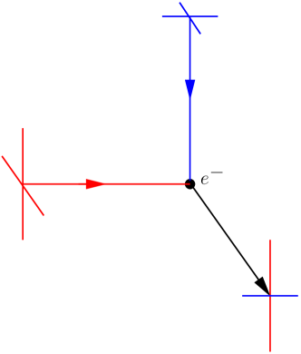
Figure 1: Polarization from Thomson scattering

Thomson scattering is proportional to the square of the scalar product $\epsilon 1.\epsilon 2$ of the incoming and outgoing photons polarizations, thus outgoing photons only carry polarization orthogonal to the scattering plane. Radiation fluxes from different directions are incoherent, therefore intensities from opposite incident directions add up and only even multipoles of the flux angular distribution contribute. In fact, only the monopole and the quadrupole remain because the scattering cross-section is quadratic in $\epsilon 1.\epsilon 2$. As $Q$ and $U$ are intensity differences, they only get contribution from the quadrupole.

Note that any polarization gets averaged out by successive rescatterings, therefore we only observe polarization from the last one, at the end of recombination. The scale of the fluctuations we can observe is of the order of the mean free path of photons when the last scattering occurs and cannot be larger than the thickness of the last scattering surface.

For density fluctuations, the local quadrupole anisotropies of the photon flux on the last scattering surface arise from velocity gradients, as sketched in figure 2. In the photon baryon fluid rest frame, the velocities of neighboring particles tend to diverge radially from and converge transversely to the scattering point when the fluid is accelerated from a hot spot (density dip, potential maximum) to a cold spot (density peak, potential dip). The reverse velocity scheme applies when the fluid is decelerated away from a cold spot. By Doppler shift, this induces a quadrupole flux anisotropy around the last scattering point, leading to radial polarization in the first case and to transverse polarization in the second case. This simple geometrical scheme does not apply to primordial gravitational waves which are quadrupolar by nature, and therefore do not need velocity gradients to generate CMB polarization.

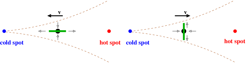
Figure 2: Polarization directions from velocity gradients. Polarization directions when the fluid is accelerated towards the cold spot (left panel) or decelerated towards a hot spot (right panel). The brown dashed curves are fluid stream lines. The small thin arrows are the fluid velocities in the fluid rest frame near the scattering point. The large thick arrows are the directions of the fluid motion near the scattering point relative to the hot and cold spots.

The above mechanism does not produce any circular polarization, and from now on, we forget about the $V$ Stokes parameter.

4 Polarized multipole expansion

As we are observing the celestial sphere, it is convenient to develop the CMB fluctuation on spherical harmonics. Because $Q\pm i\,U$ are spin 2 objects, they must be developed on spin 2 spherical harmonics [10]:

$$(Q\pm i\,U)(\vec{n})=\sum_{l\geq 2,\ |m|\leq l}a_{\pm 2lm}\,{}_{\pm 2}Y_{l}^{m}(\vec{n})$$ (3)

From these spin 2 objects, one can construct 2 real scalar quantities with opposite behavior under parity transformations:

$$\begin{array}[]{l}E(\vec{n})=\sum_{l\geq 2,\ |m|\leq l}a^{E}_{l\,m}\,Y_{l}^{m}(\vec{n})\qquad\mbox{ with positive parity}\\ B(\vec{n})=\sum_{l\geq 2,\ |m|\leq l}a^{B}_{l\,m}\,Y_{l}^{m}(\vec{n})\qquad\mbox{ with negative parity},\end{array}\ \ \mbox{ where }\ \ \begin{array}[]{l}a^{E}_{l\,m}=-\frac{a_{2lm}+a_{-2lm}}{2}\\ a^{B}_{l\,m}=i\frac{a_{2lm}-a_{-2lm}}{2}.\end{array}$$ (4)

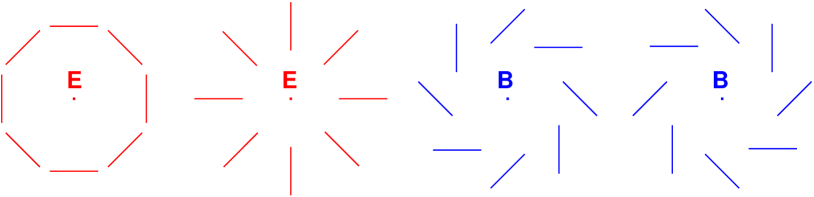
Figure 3: Typical $E$ or $B$ type polarization patterns. The opposite transformation properties under reflection appear clearly (adapted from Zaldarriaga [13]).

The different parity properties of $E$ and $B$ type polarization fluctuation are illustrated in figure 3. They arise from different parity properties of the velocity gradients, and trace the geometrical properties of the underlying fluctuations.

Including polarization, the statistical properties of Gaussian CMB fluctuations are characterized by four power spectra:

$$C^{TT}_{l}=\langle{a^{T}_{lm}}^{*}a^{T}_{lm}\rangle,\qquad C^{ET}_{l}=\langle{a^{E}_{lm}}^{*}a^{T}_{lm}\rangle,\qquad C^{EE}_{l}=\langle{a^{E}_{lm}}^{*}a^{E}_{lm}\rangle,\qquad C^{BB}_{l}=\langle{a^{B}_{lm}}^{*}a^{B}_{lm}\rangle$$ (5)

An example of the four expected spectra as predicted by the best model compatible with the results of the WMAP experiment [14] is displayed on figure 4. Notice that, because of the negative parity of $B$, its cross power spectra with both $T$ and $E$ are expected to vanish.

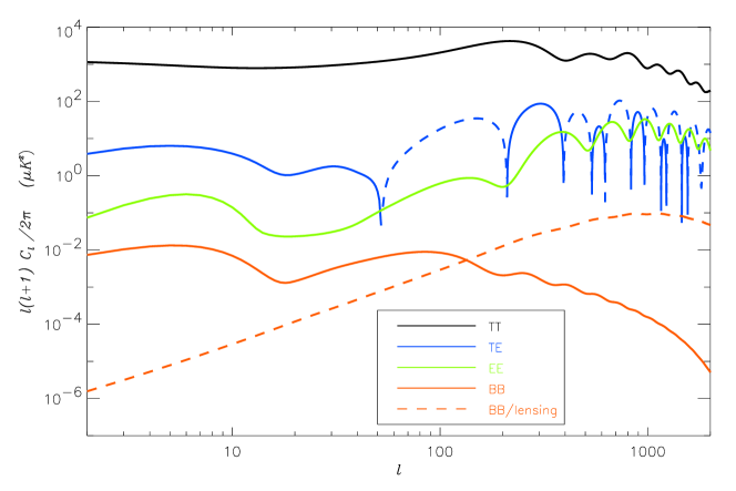
Figure 4: The four observable spectra $TT,\ TE,\ EE,\ BB$. The $TE$ spectrum can be negative (dotted segments), and apparent cusps occur when $TE$ changes sign. They correspond to the compression and expansion extrema of the $TT$ spectrum, when the fluid velocity vanishes. Note that the $EE$ spectrum is in phase opposition relative to $TT$. These spectra have been computed using the code CMBFAST [15] (http://www.cmbfast.org).

5 Information carried by CMB polarization

The CMB temperature fluctuations are the imprint on the last scattering surface of density and metric perturbations. They are classified as “scalar”, “vector” and “tensor” depending on their transformation properties under rotations. Vector perturbation get damped by expansion and only the scalar and tensor ones survive. The scalar contributions comprise total density fluctuations, also called curvature or adiabatic perturbations, and isocurvature fluctuations where only the relative densities of the different components vary. Tensor fluctuations are expected from the primordial gravity waves predicted in the inflationary scenario. CMB polarization allows to separate them from scalar perturbations (see e.g. [16, 13]).

E polarization: scalar fluctuations. Scalar perturbations only generate positive parity polarization patterns, and therefore can only produce $E$ type CMB polarization fluctuations. In the absence of isocurvature perturbations, the $TE$ spectrum is completely calculable from the $EE$ spectrum. This property is extremely well verified by the $TE$ spectrum observed by the WMAP collaboration (Figure 5).

Figure 5: The $TE$ spectrum as observed by WMAP. The solid line is computed from the best fit to the $TT$ spectrum, without additional free parameter, assuming adiabatic perturbations (Figure from reference [17], reproduced with permission of the AAS).

B Polarization: tensor fluctuations. On the contrary, tensor fluctuation can produce both $E$ and $B$ polarization [18, 19]. Therefore the relative intensity of B polarization modes is a constraint on the ratio $r$ of tensor to scalar fluctuations.

5.1 Link with the inflation paradigm

The inflation paradigm was introduced by Guth [21], Linde [22] and Albrecht & Steinhardt [23] to solve the horizon problem: the present observed Universe appears homogeneous on scales which have never been in causal contact, due to the finite light speed. In particular the CMB is homogeneous across the whole sky at the $10^{-5}$ level, although the “horizon” size at the time of decoupling is of order 1 degree on the sky sphere.

In inflationary models, the very early Universe undergoes a rapid expansion phase driven by the vacuum energy of some scalar field. This inflation must last long enough for the comoving size of the horizon before inflation to be larger than the present size of the horizon ($\simeq 1/H_{0}$). This implies an inflation factor of order $e^{40}$ to $e^{60}$, depending on when inflation ends (after GUT symmetry breaking and before baryogenesis).

Although the horizon problem, the near flatness of our universe and the elimination of unwanted relics (GUT’s monopoles, domain walls …) were the original motivations to propose inflation, this scenario also naturally provides the seeds of the present large scale structures. These seeds are the microscopic quantum fluctuations of the inflaton field, which are inflated to macroscopic adiabatic scalar perturbations during inflation. One of the generic predictions of inflation is the presence of acoustic peaks in the $C_{l}$ spectrum which have now been observed beyond any doubt [24, 25, 26, 27]. The reason is that perturbations begin to oscillate when they enter the horizon and all perturbations with the same size do so at the same time. The acoustic peaks arise from this coherent oscillation. The fact that the peaks in the $TE$ spectrum observed by WMAP are out of phase with the temperature peaks is a further confirmation of the acoustic scenario because polarization originates in velocity gradients. The dip in the $TE$ spectrum around $l\simeq 150$ indicates the presence of superhorizon size fluctuations at the time of decoupling, which is a strong indication in favor of inflation.

In much the same way, the space metric also undergoes quantum fluctuations which produce primordial gravity waves (tensor perturbations). The ratio between tensor and scalar perturbations, defined as $r=\left.\frac{C_{l}^{T}}{C_{l}^{S}}\right|_{l=2}$, is related to the energy scale of inflation $E_{\mathrm{inflation}}$. For example in the popular “slow-roll” approximation (see e.g. [20]),

$$r=0.1\,\left(\frac{E_{\mathrm{inflation}}}{2.\,10^{16}\,GeV}\right)^{4}$$

Therefore, detection of $B$-mode polarization will allow to measure this energy scale, but the quick decrease of $r$ with $E_{\mathrm{inflation}}$ may make it difficult. The primordial $BB$ spectrum in figure 4 (solid red line) corresponds to $r=0.1$.

6 Distortions by foregrounds

The polarized CMB spectra will be affected by various foregrounds. Apart from those related to galactic dust an synchrotron emission, which we shall not discuss here, some foreground effects, such as reionization and gravitational lensing, have an important cosmological significance.

6.1 Reionization

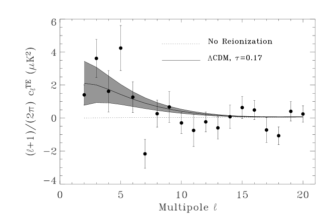
Figure 6: Zoom on the low $l$ region of the $TE$ spectrum as observed by WMAP. Dotted line: $\Lambda$CDM model with no reionization. Solid line: $\Lambda$CDM plus a reionization optical depth $\tau=0.17$. Grey area: the one sigma uncertainty from cosmic variance (Figure from reference [17], reproduced with permission of the AAS).

It has been known for a long time [28] that the universe is observed to be ionized, at least up to a redshift of $z\simeq 6$ (see e.g. [29]). This reionization is expected from the high energy photons produced in the collapse of the first generation of stars (for recent reviews, see [30]) and [31]). Present estimations place the beginning of reionization somewhere between $z=7$ and $z=30$ [16]. Reionization distorts the spectrum of CMB perturbations: free electrons re-scatter the CMB photons, diluting somewhat the temperature fluctuations. Exactly as on the last scattering surface, the local CMB quadrupole causes the rescattered CMB photons to be polarized. Because photons stream freely between their last scattering at recombination and their rescattering on reionized electrons, the polarized CMB fluctuations from reionization appear at larger scale, and therefore induce a low $l$ peak in the polarized power spectra. This reionization bump, below $l=20$, carries rich information on the reionization history of the universe [32, 33, 34]. The low $l$ peak appears on the $TE$, $EE$, $BB$ spectra in figure 4, where the reionization optical depth has been assumed to be 0.17 [17]. The WMAP experiment [14, 17] has claimed a first detection of polarization from reionization in the $TE$ spectrum (figure 6). They evaluate the reionization optical depth to be $\tau=0.17\pm 0.04$, larger than expected. This would be well described by an early reionization at redshift $11<z_{r}<30$ at the 95% confidence level. These results have trigered much work on early reionization, see for instance [35, 36, 37, 38, 39]. Forthcoming results of WMAP on the $EE$ spectrum will allow more precise statements. Future high precision measurements of large scale CMB polarization will be a very useful tool to understand early star formation.

6.2 Lensing of primordial polarized fluctuations: small scale B modes

One of the main distortions of the polarized CMB fluctuations spectrum arises from the lensing of the CMB photons by matter inhomogeneities on their way to us [40, 41]. Lensing does not produce nor rotate polarization, but deflection changes its spatial patterns. In particular it blurs the parity properties, thereby leaking $E$ modes into $B$ modes [42]. In figure 4, the dashed red line represents the $BB$ spectrum expected from lensing. One can see that it dominates at small scale and will do so at large scale if the energy scale of inflation is too low. Knox and Song [43], and independently Kesden, Cooray and Kamionkowski [44] have recently shown that $B$ modes from primordial gravity waves will be masked by lensing $B$ modes if the energy scale of inflation lies below $3.2\,10^{15}$ GeV.

Lensing of the CMB should not be only considered as a nuisance to be subtracted. It can be used as a tool to study the mass distribution between us and the last scattering surface. Hu and Okamoto [46, 47] and also Kesden, Cooray, and Kamionkowski [48] have devised an approach which treats the CMB statistically, but considers the foreground lensing potential as fixed. The breaking of anisotropy allows to consider $TB$ and $EB$ correlations which, combined with the the usual ones, can be used to reconstruct the lensing potential. This may provide a powerful tool to investigate the high redshift mass distribution.

7 Conclusion

The flatness of the universe and the harmonic structure of the CMB spectrum are now well established. The first observations of CMB polarization by DASI [49] and WMAP [17] point in the direction of inflation. We have seen that CMB polarization observations have a high potential to assess the cosmological scenario and in particular have much to say about inflation. Moreover, it carries information on early star formation and high redshift matter distribution. New results on all these issues will soon come from observations in progress or in preparation, see [3] in this issue.

We would like to thank François-Xavier Desert for many useful suggestions.

References

- [1] M.J. Rees. Polarization and spectrum of the primeval radiation in an anisotropic universe. ApJ, 153:L1, 1968.
- [2] M. M. Basko and A. G. Polnarev. Polarization and anisotropy of the RELICT radiation in an anisotropic universe. MNRAS, 191:207–215, April 1980.
- [3] J. Delabrouille, J. Kaplan, M. Piat, and C. Rosset. Polarization experiments. In The Cosmic Microwave Background: present status and cosmological perspectives, This issue of C. R. (Physique). Academie des Sciences, Paris, 2003.
- [4] S. Chandrasekhar. Radiative Transfer. Dover Publications, 1960.
- [5] J. D. Jackson. Classical Electrodynamics. John Wiley & Sons, 3rd edition, 1999.
- [6] M. Born and E. Wolf. Principles of Optics. Pergamon Press, 7th edition, 2000.
- [7] A Kosowsky. Cosmic Microwave Background Polarization. Annals Phys., 246:49, 1996.
- [8] M. Zaldarriaga and U. Seljak. An All-Sky Analysis of Polarization in the Microwave Background. Phys. Rev. D, 55:1830, 1997.
- [9] A. Cooray, A. Melchiorri, and J. Silk. Is the Cosmic Microwave Background Circularly Polarized? Phys.Lett. B, 554:1, 2003.
- [10] J.N. Goldberg et al. Spin-s Spherical Harmonics and ́. Jour. Math. Phys., 8:2155, 1967.
- [11] W. Hu and M. White. A CMB Polarization Primer. New Astronomy, 2:323, 1997.
- [12] M. Zaldarriaga. The nature of the E-B decomposition of CMB polarization. Phys.Rev., D64:103001, 2001.
- [13] M. Zaldarriaga. The Polarization of the Cosmic Microwave Background, volume Vol 2: Measuring and modelling the universe of Carnegie Observatories Astrophysics Series. Cambridge University Press, 2003. astro-ph/0305272.
- [14] C.L. Bennett et al. First Year Wilkinson Microwave Anisotropy Probe (WMAP) Observations: Preliminary Maps and Basic Results. ApJS, 148, 2003.
- [15] U. Seljak and M. Zaldarriaga. A line of sight approach to Cosmic Microwave Background anisotropies. ApJ, 469:437, 1996.
- [16] W. Hu. CMB Temperature and Polarization Anisotropy Fundamentals. Annals Phys., 303:203, 2003.
- [17] A. Kogut et al. Wilkinson Microwave Anisotropy Probe (WMAP) First Year Observations: TE Polarization. ApJS, 148, 2003.
- [18] U. Seljak and M. Zaldarriaga. Signature of Gravity Waves in Polarization of the Microwave Background. Phys.Rev.Lett., 78:2054, 1997.
- [19] M. Kamionkowski and A. Kosowsky. Detectability of Inflationary Gravitational Waves with Microwave Background Polarization. Phys.Rev., D57:685, 1998.
- [20] A. R. Liddle and D. H. Lyth. Cosmological inflation and large-scale structure. Cambridge University Press, 2000.
- [21] A. H. Guth. Inflationary universe: A possible solution to the horizon and flatness problems. Phys. Rev. D, 23:347, 1981.
- [22] A.D. Linde. A new inflationary universe scenario: a possible solution of the horizon, flatness, homogeneity, isotropy, and primordial monopole problems. Phys. Lett., 108B:389, 1982.
- [23] A. Albrecht and P. J. Steinhardt. Cosmologie for grand unified theories with radiation induced symmetry breaking. Phys. Rev. Lett., 48(1220), 1982.
- [24] C. B. Netterfield, M. J. Devlin, N. Jarolik, L. Page, and E. J. Wollack. A Measurement of the Angular Power Spectrum of the Anisotropy in the Cosmic Microwave Background. ApJ, 474:47, January 1997.
- [25] S. Hanany et al. MAXIMA-1: A Measurement of the Cosmic Microwave Background Anisotropy on Angular Scales of 10’-5. ApJL, 545:L5, December 2000.
- [26] P. de Bernardis et al. A flat Universe from high-resolution maps of the cosmic microwave background radiation. Nature, 404:955–959, April 2000.
- [27] A. Benoît et al. The Cosmic Microwave Background Anisotropy Power Spectrum measured by Archeops. A&A, 399:L19, 2003.
- [28] J. E. Gunn and B. A. Peterson. On the Density of Neutral Hydrogen in Intergalactic Space. ApJ, 142:1633, 1965.
- [29] A. Loeb and R. Barkana. The Reionization of the Universe by the First Stars and Quasars. ARA&A, 39:19, 2001.
- [30] Barkana and A. Loeb. In the Beginning: The First Sources of Light and the Reionization of the Universe. Phys. Rep., 349:125, 2001.
- [31] J. Miralda-Escude. The Dark Age of the Universe. Science, 300:1904, 2003.
- [32] M. Zaldarriaga. Polarization of the Microwave Background in reionized models. Phys.Rev.D, 55:1822, 1997.
- [33] M. Kaplinghat, M. Chu, Z. Haiman, G. P. Holder, L. Knox, and C. Skordis. Probing the Reionization History of the Universe using the Cosmic Microwave Background Polarization. ApJ, 583:24–32, January 2003.
- [34] G. Holder, Z. Haiman, M. Kaplinghat, and L. Knox. The Reionization History at High Redshifts II: Estimating the Optical Depth to Thomson Scattering from CMB Polarization. to appear in ApJ, 2003.
- [35] W. Hu and G.P. Holder. Model-Independent Reionization Observables in the CMB. Phys.Rev., D68:023001, 2003.
- [36] R. Barkana and A. Loeb. GRBs versus Quasars: Lyman-alpha Signatures of Reionization versus Cosmological Infall. submitted to ApJ, 2003. astro-ph/0305470.
- [37] L. Knox. CMB Signatures of Extended Reionization. In S. Hanany and K.A. Olive, editors, ”The Cosmic Microwave Background and its Polarization”, To appear in New Astronomy Reviews, 2003. astro-ph/0305588.
- [38] S. Peng Oh and Z. Haiman. Fossil HII Regions: Self-Limiting Star Formation at High Redshift. Submitted to MNRAS, 2003. astro-ph/0307135.
- [39] Ch. A. Onken and Jordi Miralda-Escude. History of Hydrogen Reionization in the Cold Dark Matter Model. submitted to ApJ, 2003. astro-ph/0307184.
- [40] U. Seljak. Gravitational Lensing Effect on Cosmic Microwave Background Anisotropies: A Power Spectrum Approach. ApJ, 463(1), 1996.
- [41] F. Bernardeau. Weak lensing detection in CMB maps. A&A, 324:15, 1997.
- [42] M. Zaldarriaga and U. Seljak. Gravitational lensing effect on Cosmic Microwave Background polarization. Phys. Rev. D, 58:23003, 1998.
- [43] L. Knox and Y.-S. Song. A limit on the detectability of the energy scale of inflation. Phys.Rev.Lett., 89:011303, 2002. astro-ph/0202286.
- [44] M. Kesden, A. Cooray, and M. Kamionkowski. Separation of Gravitational-Wave and Cosmic-Shear Contributions to Cosmic Microwave Background Polarization. Physical Review Letters, 89(1):011304, July 2002.
- [45] W.H. Kinney. The energy scale of inflation: is the hunt for the primordial B-mode a waste of time? In S. Hanany and K.A. Olive, editors, The Cosmic Microwave Background and its Polarization, To appear in New Astronomy Reviews, 2003. astro-ph/0307005.
- [46] W. Hu and T. Okamoto. Mass Reconstruction with CMB Polarization. ApJ, 574:566, 2002.
- [47] T. Okamoto and W. Hu. CMB Lensing Reconstruction on the Full Sky. Phys. Rev., D67:083002, 2003.
- [48] M. Kesden, A. Cooray, and M. Kamionkowski. Lensing Reconstruction with CMB Temperature and Polarization. Phys.Rev., D67:123507, 2003.
- [49] J. M. Kovac, E. M. Leitch, C. Pryke, J. E. Carlstrom, N. W. Halverson, and W. L. Holzapfel. Detection of polarization in the cosmic microwave background using DASI. Nature, 420:772, 2002.