Curvature radiation in pulsar magnetospheric plasma

Abstract

We consider the curvature radiation of the point-like charge moving relativistically along curved magnetic field lines through a pulsar magnetospheric electron-positron plasma. We demonstrate that the radiation power is largely suppressed as compared with the vacuum case, but still at a considerable level, high enough to explain the observed pulsar luminosities. The emitted radiation is polarized perpendicularly to the plane of the curved magnetic filed lines coincides with that of extraordinary waves, which can freely escape from the magnetospheric plasma. Our results strongly support the coherent curvature radiation by the spark-associated solitons as a plausible mechanism of pulsar radio emission.

1 Introduction

Although almost 35 years have passed since the discovery of pulsars, the mechanism of their radio emission still remains unknown. This is one of the most difficult problems of modern astrophysics. Soon after discovery, curvature radiation was suggested as a plausible mechanism for the observed pulsar radio emission (Radhakrishnan & Cooke, 1969; Komesaroff, 1970; Ruderman & Sutherland, 1975). In fact, curvature radiation is the most natural and practically unavoidable emission process in pulsar magnetosphere. Most of the pulsar models suggest creation of dense electron-positron plasma near the polar cap. These charged particles move relativistically with Lorentz factors $\gamma\sim 10^{2}-10^{3}$ along dipolar magnetic field lines. Therefore, they emit curvature radiation at the characteristic frequencies $\nu_{c}\sim\gamma^{3}c/r_{c}$, where $r_{c}$ is the radius of curvature of field lines, which falls into the observed pulsar radio band if $r_{c}\sim 10^{8}-10^{9}$ cm. This is a typical value of the radius of curvature of dipolar field lines at altitudes of about $10^{7}-10^{8}$ cm, where the observed pulsar radio emission is supposed to originate (Kijak & Gil, 1998, and references therein).

However, some serious problems are encountered while considering the curvature radiation in pulsars. The first, and probably the most important one, is related with coherency of the pulsar radiation. It is well known that the incoherent sum of a single particle curvature radiation is not enough to explain a very high brightness temperature of pulsar radio emission. Therefore, one is forced to postulate the existence of charged bunches containing at least $10^{15}$ electron charges in a small volume that can radiate the coherent curvature emission. However, it is not easy to form such charge bunches (see Melrose, 1992, for review). Moreover, even if a bunch can be formed, it is not automatic that it will emit coherent radiation. For example, bunches formed naturally by linear electrostatic waves (e.g. Ruderman & Sutherland, 1975) cannot provide any emission (Melikidze, Gil & Pataraya, 2000, hereafter MGP00, and references therein). The natural mechanism for the formation of charged bunches was first proposed by Karpman et al. (1975), who argued that the modulational instability in the turbulent plasma generates charged solitons, provided that species of different charge have different masses. Such charged solitons were observed in the laboratory electron-ion plasma (Sagdeev, 1976) and perhaps even in the Earth ionosphere (Petviashvili, 1976). In pulsar magnetospheric plasma, distribution functions of electrons and positrons are different, because plasma screens the electric field induced by co-rotation (Scharlemann, 1974; Cheng & Ruderman, 1977). This causes the effective relativistic masses of electrons and positrons to be different, which can result in a net charge of solitons formed in pulsar magnetosphere (Melikidze & Pataraya, 1980, 1984, MGP00). The net soliton charge can also be induced by admixture of ions in the plasma flow above the polar cap (Cheng & Ruderman, 1980; Gil, Melikidze & Geppert, 2003). One should mention here that to explain coherent radio emission we do not necessarily need stable solitons but only large scale (as compared with Langmuir wavelength) charge density fluctuations.

The second problem is related to the fact that the bunches (solitons) are surrounded by the magnetized plasma, which strongly affects the radiation process. The soliton size, which is determined by the level of the turbulence, is evidently larger than the wavelength of the Langmuir waves. A bunch is unable to emit radiation with the wavelength shorter than its longitudinal size. Therefore, the soliton should emit only at frequencies $\omega$ below the frequency of the plasma waves. In the pulsar frame of reference, the corresponding condition writes $\omega<2\sqrt{\gamma}\omega_{p}$, where $\gamma$ is the Lorentz factor of plasma motion, $\omega_{p}=(4\pi e^{2}n/m)^{1/2}$ is the plasma frequency, $n$ is the total number density of electrons and/or positrons, $e$ is and $m$ is the charge and the mass of electron, respectively. Since at the expected emission altitudes $\nu_{p}=\omega_{p}/2\pi\sim 1$ GHz (see eq. [3] in MGP00) and $\gamma\sim 10^{2}$, the coherent radiation should be emitted at frequencies $\nu\raisebox{-1.29167pt}{\mbox{$\stackrel{{\scriptstyle<}}{{{}_{\sim}}}\,$}}20$ GHz, as observed in radio pulsars.

There are three waves propagating in the pulsar plasma: the extraordinary wave $(\omega\approx kc)$ polarized perpendicularly to the plane set by the ambient magnetic field and the wave vector $k$, and the two ordinary waves polarized in this plane, that is, the superluminal wave $(\omega>kc)$ and subluminal wave $(\omega<kc)$. Under the condition $\omega<2\sqrt{\gamma}\omega_{p}$, emission of the superluminal wave is heavily suppressed by the Razin effect (Razin, 1960). The subluminal wave may, in principle, be emitted, but it cannot escape from the plasma. In fact, it is ducted along the curved magnetic field lines preserving direction of the wave vector and eventually decays as a result of the Landau damping (Barnard & Arons, 1986). The extraordinary wave escapes freely but in the infinitely strong, straight magnetic field it cannot be emitted because it does not interact with the plasma particles. However, in the curved magnetic field such wave can be emitted like in the vacuum case, in which a significant fraction of the curvature emission is polarized perpendicularly to the magnetic field line plane (e.g. Jackson, 1975; Gil & Snakowski, 1990).

The aim of this paper is to calculate the curvature radiation within the plasma under condition

$$\varepsilon\equiv\frac{\omega^{2}}{4\gamma\omega_{p}^{2}}\ll 1.$$ (1)

We consider emission from a point charge (modelling a small soliton/bunch) moving circularly in the cylindrically symmetric background. The magnetic field, which is assumed to be infinitely strong, has circular field lines, and the electron-positron plasma moves relativistically (with Lorentz factor $\gamma$) along these field lines. We find that the point charge emits curvature radiation in the extraordinary mode. The power of this radiation is suppressed by a factor $\varepsilon$ (eq. [1]), as compared with the vacuum case but still remains rather high. It was found recently that the Vela pulsar emits radio waves polarized predominantly in the direction perpendicular to the plane of dipolar magnetic field lines (Lai et al., 2001), strongly suggesting that these are escaping extraordinary waves. Our results demonstrate that such radiation can be generated within the pulsar magnetosphere by means of the coherent curvature radiation. This radiation can also leave the magnetospheric plasma and reach a distant observer.

MPG00 proposed the spark-associated soliton model for pulsar radio emission, in which the charged solitons are formed by nonlinear evolution of plasma waves triggered by a sparking discharge of a high accelerating potential drop above the polar cap. These relativistic solitons emit the coherent curvature radio emission at altitudes of about 50 stellar radii in typical pulsars. The total luminosities emitted by an ensamble of solitons are consistent with the observed pulsar fluxes. The formation of charged solitons in pulsar magnetosphere, as well as their coherent curvature radiation, is well justified by MGP00. The only deficiency of this model is that the curvature radiation was calculated in vacuum approximation. We argue in this paper that the soliton coherent curvature radiation is still a plausible mechanism of the observed pulsar radio emission even when the presence of the ambient plasma is taken into account.

2 Wave equations

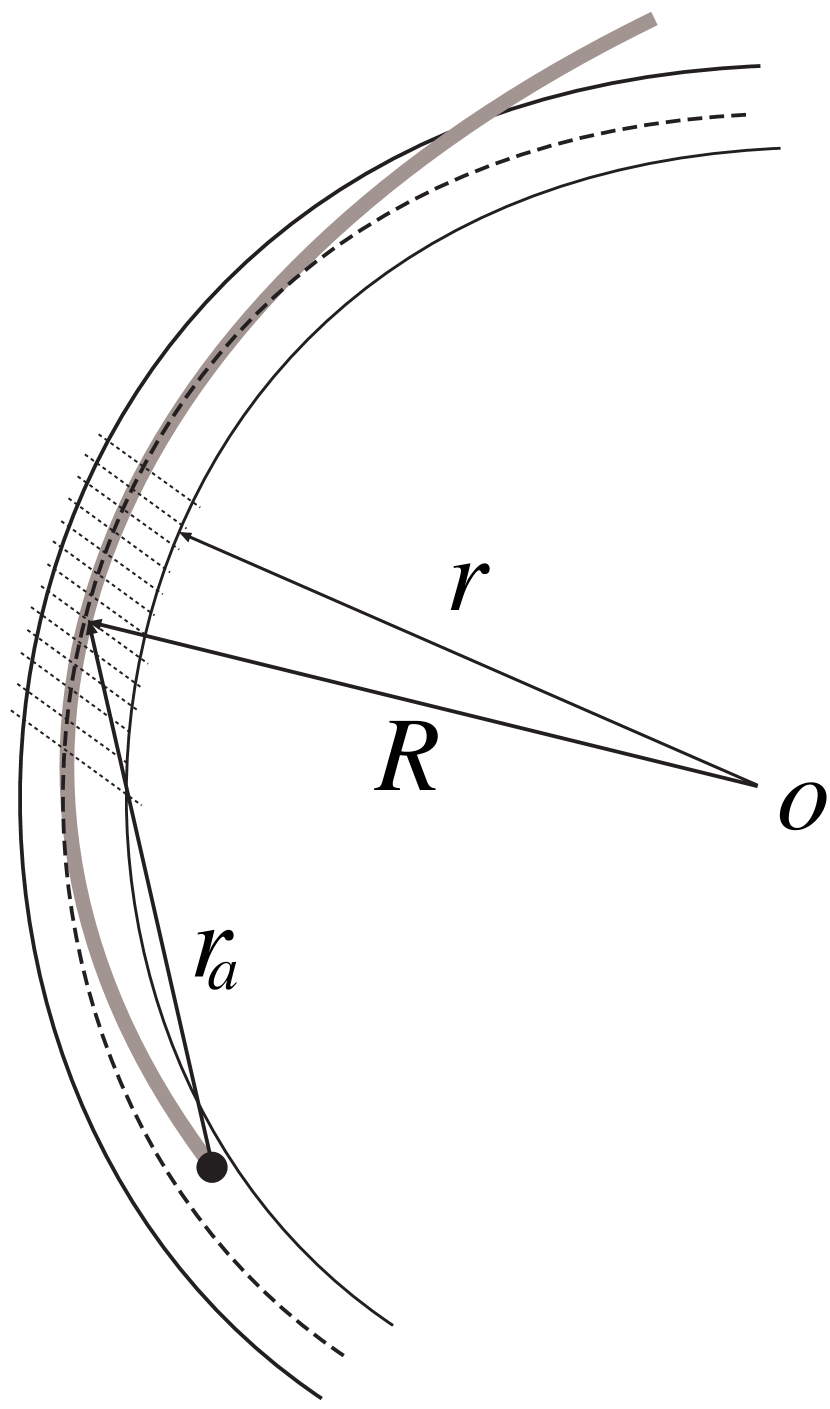
Figure 1: Schematic picture of the radiation region (marked by dotted parallel lines) and the system of cylindrical coordinates $(r,\theta,z)$, with $z$-axis directed upright to the plane of the figure. The charged particle moves along the dashed circle with radius $R$, which is locally tangent to a dipolar magnetic field line marked by a thick shadowed line. The thick black dot represents the pulsar and $r_{a}$ is radio emission altitude.

We now examine the curvature radiation from the point-like charge moving relativistically along a curved trajectory within the electron-positron plasma. We find the radiation power by calculating the work done on this charge by the excited electromagnetic field (e.g. Melrose, 1980). It is convenient to considered the curvature radiation in the cylindrical coordinates $(r,\theta,z)$. The force lines of the infinitely strong magnetic field are assumed to be concentric arcs with the radius of curvature $r$ being much larger than the size of the considered region of emission, marked by dotted parallel lines in Figure 1. The charged particle moves along the dashed circle with radius R. The thick shadowed line represents the actual magnetic field lines, which are locally modelled by concentric arcs. The thick dot represents the pulsar and $r_{a}$ is a radio emission altitude.

The wave equation for the electromagnetic vector potentials writes

$${\frac{1}{c^{2}}}\frac{\partial^{2}\mbox{\boldmath$A$}}{\partial t^{2}}+\triangle{\mbox{\boldmath$A$}}=-\frac{4\pi}{c}\mbox{\boldmath$J$},$$ (2)

provided that vector and scalar potentials are subject to the Lorentz gauge condition

$${\frac{1}{c}}\frac{\partial\Psi}{\partial t}+{{\bf\nabla}\cdot\mbox{\boldmath$A$}}=0.$$ (3)

The scalar potential $\Psi$ satisfies the wave equation as well, provided that the total charge of the system is conserved. The electric field of the wave is defined as

$$\mbox{\boldmath$E$}=-{\frac{1}{c}}\frac{\partial\mbox{\boldmath$A$}}{\partial t}-\nabla\Psi.$$ (4)

We use equations (2) and (3) as a complete system of equations. Let us note that in the infinitely strong magnetic field the particles are forced to move exclusively along the field lines and, consequently, the current can be excited only along the $\theta$-direction.

Making the Fourier transform

$$f(r,s,k_{z},\omega)=\int\exp(i\omega t-is\theta-ik_{z}z)f(r,\theta,z,t)dtd\theta dz,$$ (5)

where $f$ denotes $\Psi$ and components of $A$, $J$ and $E$, we get the following set of equations

$$\Psi=s\frac{c}{\omega r}A_{\theta}+\frac{k_{z}c}{\omega}A_{z}-i\frac{c}{\omega r}\frac{\partial}{\partial r}rA_{r};$$ (6)

$$\frac{\partial}{\partial r}\frac{1}{r}\frac{\partial}{\partial r}rA_{r}+\left(\frac{\omega^{2}}{c^{2}}-\frac{s^{2}}{r^{2}}-k^{2}_{z}\right)A_{r}-2i\frac{s}{r^{2}}A_{\theta}=0;$$ (7)

$$\frac{\partial}{\partial r}\frac{1}{r}\frac{\partial}{\partial r}rA_{\theta}+\left(\frac{\omega^{2}}{c^{2}}-\frac{s^{2}}{r^{2}}-k^{2}_{z}\right)A_{\theta}+2i\frac{s}{r^{2}}A_{r}=-\frac{4\pi}{c}J_{\theta};$$ (8)

$$\frac{\partial}{\partial r}\frac{1}{r}\frac{\partial}{\partial r}rA_{z}+\left(\frac{\omega^{2}}{c^{2}}-\frac{s^{2}}{r^{2}}-k^{2}_{z}\right)A_{z}=0.$$ (9)

One should remember that according to the Landau prescription, $\omega$ is assumed to have a small positive imaginary part. We do not write down it explicitly here but will restore it in the appropriate place (see bellow eq. [24]).

Now we need to find the current density associated with the point charge $J^{\rm part}$ and current density $J^{\rm plasma}$ excited in plasma by the wave. If we assume that the emitting particle rotates with the velocity $V$ (the corresponding Lorentz factor is $\Gamma$) along a circle with the radius $R$, we can introduce the corresponding current density as $j_{\theta}=(QV/R)\delta(r-R)\delta(\theta-Vt/R)\delta(z)$, where $Q$ is a charge of the emitting particle. Making the Fourier transform we get

$$J^{\rm part}_{\theta}=2\pi Q\frac{V}{R}\delta(r-R)\,\delta\!\left(\omega-s\frac{V}{R}\right).$$ (10)

In the infinitely strong magnetic field, only $\theta$-component of the electric field of the emitted wave excites the currents in the plasma. Assuming that the plasma is cold and moves with the velocity $v$, we get

$$J^{\rm plasma}_{\theta}=i\frac{\omega_{p}^{2}}{4\pi}\frac{1}{\gamma^{3}}\frac{\omega}{\left(\omega-s\,\frac{v}{r}\right)^{2}}E_{\theta},$$ (11)

(see details in Appendix A). Here $\gamma=(1-v^{2}/c^{2})^{-1/2}$ in the plasma Lorentz factor. The Fourier component of the longitudinal electric field (eq. [4]) can be expressed via the potentials in the form

$$E_{\theta}=i\left(\frac{\omega}{c}A_{\theta}-\frac{s}{r}\Psi\right).$$ (12)

Our objective is to find such solution of equations (6–12), which remains finite as $r\to 0$ and comprises an outgoing wave as $r\to\infty$.

3 Short wavelength approximation

Ultrarelativistic particles emit waves with the wavelength much shorter than the curvature radius of their trajectory. Therefore, we can solve the wave equations in the short wave approximation, $\omega r/c\sim s\gg 1$. Let us start with the so-called WKB approximation, in which $A\propto\exp(i\int k_{r}dr)$ and therefore the solution splits into two waves

$$k_{r}^{2}=\frac{\omega^{2}}{c^{2}}-\frac{s^{2}}{r^{2}}-k_{z}^{2}$$ (13)

and

$$\omega^{2}-\left(\frac{s^{2}}{r^{2}}+k_{z}^{2}+k_{r}^{2}\right)c^{2}=\frac{\omega_{p}^{2}}{\gamma^{3}(\omega-s\frac{v}{r})^{2}}\left(\omega^{2}-\frac{s^{2}}{r^{2}}c^{2}\right).$$ (14)

Equation (13) describes the extraordinary wave ($\omega=kc$) polarized perpendicularly to the plane set by the local magnetic field and $k$ vector, while the ordinary wave polarized in this plane is described by equation (14). Under the condition expressed by equation (1), equation (14) has a solution corresponding to the nearly transverse wave with the dispersion law in the form

$$\omega^{2}=\left(\frac{s}{r}c\right)^{2}\left(1-\frac{\left(k_{r}^{2}+k_{z}^{2}\right)c^{2}}{4\gamma^{2}\omega_{p}^{2}}\right)\;\;{\rm if}\;\;\left(k_{r}^{2}+k_{z}^{2}\right)c^{2}<<\omega_{p}^{2}.$$ (15)

The WKB approximation is not valid close to the classical reflection radius $r_{0}$, defined as

$$\omega^{2}-\frac{s^{2}}{r_{0}^{2}}c^{2}-k^{2}_{z}c^{2}=0.$$ (16)

At $r\approx r_{0}$, the refraction indices $N\equiv kc/\omega$ of extraordinary (eq. [13]) and ordinary (eq. [15]) waves are very close to each other ($\omega=kc$), thus providing conditions for the wave coupling. In this region $k_{r}$ goes to zero, thus forming a caustic zone.

Consequently, we should solve differential equations (6–12) for the electromagnetic potentials in the region $r\approx r_{0}$ and then match the obtained solution with the appropriate WKB solution (Eqs. [13] or [14]). Note that because the particle emits nearly along the local magnetic field, the radius of the particle trajectory $R$ should be also close to $r_{0}$. It is therefore convenient to use the radial variable

$$x\equiv\frac{r-r_{0}}{r_{0}}s^{2/3}.$$ (17)

In the region of interest $x\sim 1$ and correspondingly $|r-r_{0}|\sim r_{0}s^{-2/3}\ll r_{0}$. The power series expansion in small $s^{-1/3}\ll 1$ allows to reduce equations (7–9) to the form

$$A_{r}^{\prime\prime}+2xA_{r}-2is^{-1/3}A_{\theta}=0,$$ (18)

$$A_{\theta}^{\prime\prime}+2xA_{\theta}-2is^{-{1}/{3}}A_{r}=D,$$ (19)

$$A_{z}^{\prime\prime}+2xA_{z}=0,$$ (20)

(see Appendix B for details), where

$$D \equiv -4\pi r_{0}^{2}s^{-{4}/{3}}\left(J_{\theta}^{\rm{plasma}}+J_{\theta}^{\rm{part}}\right)$$ (21)

$$= 8\frac{\omega_{p}^{2}\gamma}{\omega^{2}}\frac{\left(2\left(x+a\right)A_{\theta}+is^{{1}/{3}}A_{r}^{\prime}\right)}{\left(1+2s^{-{2}/{3}}\gamma^{2}\left(a+x\right)\right)^{2}}-8\pi^{2}VQs^{-{2}/{3}}\delta\left(x-X\right)\delta\left(\omega-s\frac{V}{R}\right),$$

$$X=-a-\frac{1}{2}\frac{s^{{2}/{3}}}{\Gamma^{2}}\;\;{\rm and}\;\;\;a=\frac{1}{2}\frac{s^{{2}/{3}}k_{z}^{2}c^{2}}{\omega^{2}},$$ (22)

where prime denotes differentiation with respect to $x$-coordinate and $X$ denotes $x$-coordinate of the emitting particle (see Appendix B). We do not assume any relationship between $A_{r}$ and $A_{\theta}$ and thus we retain terms proportional to a small factor $s^{-1/3}$ in equations (18) and (19).

The gauge condition expressed by equation (3) still permits a gauge transformation $\Psi\to\Psi-\partial\Phi/\partial t$, ${\mbox{\boldmath$A$}}\to{\mbox{\boldmath$A$}}+\nabla\Phi$, provided that $\Phi$ satisfies d’Alembert’s equation, which reduces to $\Phi^{\prime\prime}+2x\Phi=0$ if $\omega r\gg 1$ and $|r-r_{0}|\ll r_{0}$. Therefore, one can choose $A_{z}=0$ (c.f. eq. [20]) and solve equations (18) and (19) together with equation (3) or equation (6). The solution must comprise an evanescent wave at $x<X$ and an outgoing wave at $x>X$.

The Green function for equations (18) and (19) can be found from the solution of the corresponding homogeneous equations matched at the point $x=X$ according to the following matching conditions

$$A_{\theta}^{\prime}(X+0)-A^{\prime}_{\theta}(X-0)=-8\pi^{2}QVs^{-2/3}\delta\left(\omega-s\frac{V}{R}\right)\;\;{\rm and}\;\;A^{\prime}_{r}(X+0)=A^{\prime}_{r}(X-0),$$ (23)

which can be obtained straightforwardly integrating equations (18) and (19) between limits $X-0$ and $X+0$.

Let us consider the first term of $D$ (see eq. [21], which is just the right hand side of eq. [19]). The nominator in this term (which according to eq. [B9] is proportional to $E_{\theta}$) should be small, due to the condition expressed by equation (1). Thus, in the zeroth approximation in $\varepsilon$ (eq. [1]) the following relationship holds

$$A_{\theta}=-i\frac{s^{1/3}}{2(x+a+i0)}A_{r}^{\prime}.$$ (24)

Here we take into account the fact that according to the Landau prescription $\omega$ and consequently $a$ have a small imaginary part. Substituting the obtained relation into equation (18) we get a closed equation for $A_{r}$. Let us note, that equation (24) means that $E_{\theta}=0$. Therefore in order to calculate the emission power we need the next approximation in $\varepsilon$ (see the next section).

Now it is convenient to introduce the dimensionless function $u(x)$ such that

$$A_{r}=\frac{8\pi^{2}QV}{s}\frac{X+a}{X}i\delta(\omega-sV/R)u,$$ (25)

(see Appendix B for details), which satisfies the following equation

$$u^{\prime\prime}-\frac{u^{\prime}}{x+a+i0}+2xu=0.$$ (26)

The matching conditions (eq. [23]) can be now reduced to

$$u(X+0)-u(X-0)=1\;{\rm and}\;u^{\prime}(X+0)-u^{\prime}(X-0)=0.$$ (27)

Equation (26) has the Airy type asymptotics $u\to\exp(\pm(2\sqrt{2}/3)ix^{3/2})$. Therefore, we should look for the solution which satisfies the conditions $u\to\exp(-(2\sqrt{2}/3)(-x)^{3/2})$ as $x\to-\infty$ and $u\to\exp(i(2\sqrt{2}/3)x^{3/2})$ as $x\to\infty$. Then we can find $A_{r}$ and $A_{\theta}$ from equations (24) and (25), and match them to the WKB solution (eq. [13]) as $x\to\infty$.

It is straightforward to calculate the electric field of the waves in the far zone using equations (4), (6) and (24) as

$$\left(E_{r},E_{\theta},E_{z}\right)\propto\left(\frac{k_{z}c}{\omega},\;0,\;-\frac{s^{1/3}}{\sqrt{2x}}\right)\exp\left(i\frac{2\sqrt{2}}{3}x^{3/2}\right).$$ (28)

This solution is valid in the region $1\ll x\ll s^{2/3}$ (see eq. [17]), where it is smoothly matched to the global WKB solution expressed by equation (13). One can see that the outgoing wave constitutes the extraordinary mode polarized predominantly in the direction perpendicular to the plane of the curved magnetic field lines.

Unfortunately equation (26) cannot be solved by using any known special functions, and has to be solved numerically. For the numerical solution, it is convenient to reduce equation (26) to the Rikkati type equation

$$w^{\prime}+w^{2}-\frac{w}{x+a+i0}+2x=0,$$ (29)

where $w=u^{\prime}/u$. We need only the imaginary part of $u$, because, as it is shown in the next section, the emissivity of the particle is expressed via ${\rm Im}u(X)$ (see eq. [31,32]). Using the matching conditions expressed by equation (27), we can express ${\rm Im}u(X)$ by the solution of equation (29), that is

$${\rm Im}u(X)=\frac{w_{-}{\rm Im}w_{+}}{(w_{-}-{\rm Re}w_{+})^{2}+({\rm Im}w_{+})^{2}}.$$ (30)

Starting from a large negative $x$ for which $w=\sqrt{2}\sqrt{-x}$ (an evanescent wave) and integrating numerically to $x=X$, we found a solution $w_{-}\equiv w(X-i0)$. On the other hand starting from a large positive $x$, for which $w=i\sqrt{2}\sqrt{x}$ (an outgoing wave) and integrating to some $x=\epsilon\ll 1$, then integrating (in the complex plane) along the semicircle $x=\epsilon\exp{i\phi}$, and finally integrating further along the real axis to the point $x=X$, we found another solution $w_{+}\equiv w(X+i0)$.

4 Emissivity of curvature radiation

The emitted power can be found by calculating the work done by the radiative electric field on the emitting particle

$$P=-\int dtd\mbox{\boldmath{$r$}}j^{\rm part}_{\theta}(t,{\bf r})E_{\theta}(t,{\bf r})$$ (31)

(e.g. Melrose, 1980). Note that $E_{\theta}=0$ in the zeroth approximation in $\varepsilon$ (see eq. [24]), therefore we should find the next approximation. It can be done easily substituting into the left hand side of equation (19) the values found in the zeroth approximation. We find that

$$E_{\theta}=2i\pi^{2}s^{-1}\Gamma^{4}\frac{k_{z}^{2}c}{\omega_{p}^{2}}\frac{Q}{\gamma}\frac{\left(1-\frac{\gamma^{2}}{\Gamma^{2}}\right)^{2}}{\left(1+\frac{k_{z}^{2}c^{2}}{\omega^{2}}\Gamma^{2}\right)}\delta\left(s-\omega\frac{R}{V}\right)u\left(x\right).$$ (32)

Now we can write the emissivity in the form

$$\eta\equiv\frac{d^{3}P}{dtd\nu d\mu}=\frac{c}{\pi}\Lambda\frac{Q^{2}\Gamma^{4}}{R^{2}}\left(1-\frac{\gamma^{2}}{\Gamma^{2}}\right)^{2}F\left(\nu,\mu\right),$$ (33)

where

$$F\left(\nu,\mu\right)=\frac{\nu^{2}\mu^{2}}{\left(1+\mu^{2}\right)}{\rm{Im}}u\left(X\right),$$ (34)

and dimensionless frequency $\nu$ and angle $\mu$ are defined as

$$\nu=\frac{\omega}{\omega_{c}}=\omega\frac{R}{c\Gamma^{3}}\;\;\;{\rm and}\;\;\;\mu=\frac{k_{z}}{k}\Gamma=\frac{k_{z}c}{\omega}\Gamma.$$ (35)

Let us note that a position $X$ of the emitting particle can be expressed by means of $\nu$ and $\mu$ as $X=-0.5\nu^{2/3}\left(1+\mu^{2}\right)$. The parameter

$$\Lambda=\frac{1}{4\gamma}\left(\frac{c\Gamma^{3}}{\omega_{p}R}\right)^{2}\ll 1$$ (36)

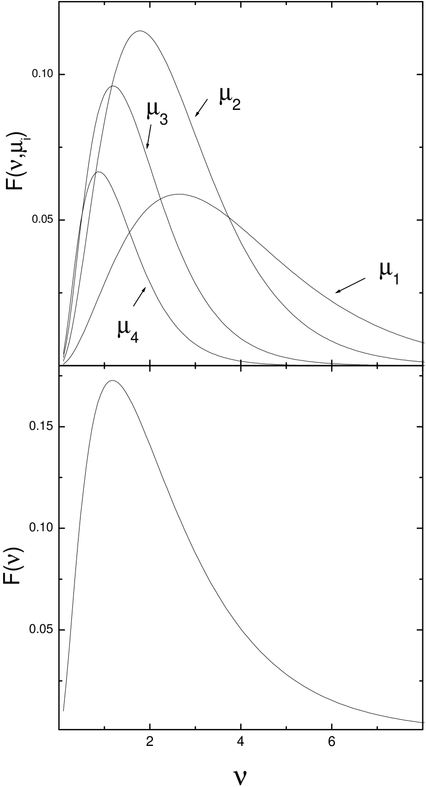
Figure 2: Distribution of the radiation power emitted in all directions $F(\nu)=\int F(\nu,\mu)d\mu$ (lower panel) and in various directions $F(\nu,\mu_{i})$ (upper panel) over the dimensionless frequency $\nu=\omega/\omega_{c}=\omega Rc^{-1}\Gamma^{-3}$, where $\mu_{1}=0.5$, $\mu_{2}=1$, $\mu_{3}=1.5$ and $\mu_{4}=2$.

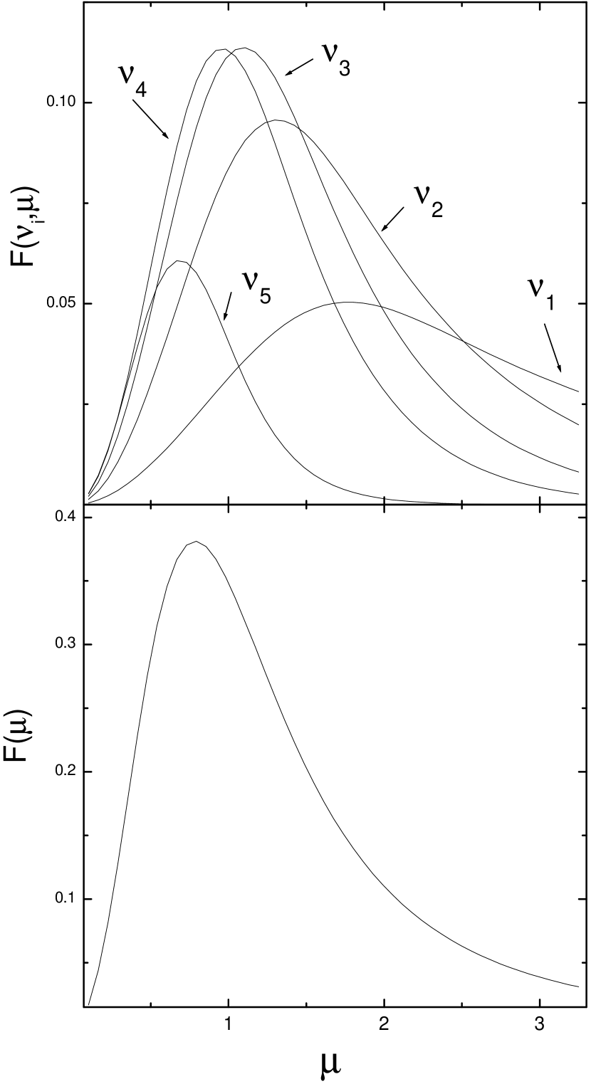
Figure 3: Distribution of the radiation power emitted at all frequencies $F(\mu)=\int F(\nu,\mu)d\nu$ (lower panel) and at various frequencies $F(\nu_{i},\mu)$ (upper panel) over the dimensionless angle $\mu=k_{z}c\Gamma/\omega$, where $\nu_{1}=0.5$, $\nu_{2}=1$, $\nu_{3}=1.5$, $\nu_{4}=2$ and $\nu_{5}=4$.

describes the suppression of the emissivity of the curvature radiation by the surrounding plasma. Actually, this is the ratio of the curvature radiation frequency to the plasma waves frequency, thus it corresponds to the condition expressed by equation (1) at the frequency $\omega=\omega_{c}\equiv c\Gamma^{3}/R$ (see also discussion below eq. [42]). As a consistency check let us note that it follows from equation (33) that $\eta=0$ if $\Gamma=\gamma$ (no radiation from uniform plasma motion), as expected. Function $F\left(\nu,\mu\right)$ is plotted in Figures 2 and 3 for various values of $\nu$ and $\mu$. Let us note that $\mu=1$ corresponds to the radiation angle $1/\Gamma$ from the plane of the source motion and $\nu=1$ corresponds to the characteristic frequency of curvature radiation $\nu_{c}=c\Gamma^{3}/2\pi R$. The polarization of this radiation is that of the extraordinary wave. The numerical values on the vertical axes in Figs. 2 and 3 can be useful in estimating the emissivity of curvature radiation of the point-like charge $Q$ moving relativistically (Lorentz factor $\Gamma$) through the relativistic plasma (Lorentz factor $\gamma$) in pulsar magnetosphere. Note that the emissivity is zero if $\mu=0$, which means that although all the radiation is concentrated within the angle $\sim 1/\Gamma$ around the plane of the charge trajectory, there is no radiation exactly in this plane.

The total luminosity from the charge can be obtained as $L_{1}=\int\eta d\mu d\nu$, where $\eta$ is the emissivity described by equation (33). One can find by numerical integration that $\int F(\mu,\nu)d\mu d\nu=0.53$ and obtain

$$L_{1}\approx 0.1\Lambda c\frac{Q^{2}\Gamma^{4}}{R^{2}}\left(1-\frac{\gamma^{2}}{\Gamma^{2}}\right)^{2}.$$ (37)

5 How can the particle emit radiation polarized perpendicularly to the plane of its trajectory?

According to our results the escaping waves are polarized almost perpendicularly to the plane of the magnetic field curvature, whereas the wave itself propagates nearly in this plane. Thus, this wave constitutes the extraordinary plasma mode. At first sight this conclusion seems counterintuitive. It is generally believed that in the infinitely strong magnetic field the extraordinary wave cannot be excited because the electric field of this wave is perpendicular to the external magnetic field and therefore it does not interact with the plasma. However, this statement is correct only in the case of the straight magnetic field. It is the curvature of field lines which makes a difference. For example (Luo, 1993) and (Luo & Melrose, 1995) demonstrated that the extraordinary mode can be generated in the infinitely strong magnetic field provided that the field lines are twisted. In this paper we show that the extraordinary mode can be excited even if the curved field lines lie in the plane, as it is in the case of a dipolar pulsar magnetic field.

To illustrate that let us consider the vacuum case first. The curvature radiation is polarized predominantly in the plane of the particle trajectory, however about 15% of the total power is emitted with the polarization perpendicular to this plane (Jackson, 1975, p. 675). Of course, the radiation which is emitted exactly in the plane of the particle trajectory is completely polarized in this plane. However, the radiation emitted at the angle about $1/\Gamma$ to the plane of the particle trajectory ($k_{z}/k\sim 1/\Gamma$) is elliptically polarized.

In the case of the plasma in the infinitely strong magnetic field, a charged particle can emit only waves with a nonzero component of the electric field along the external magnetic field. According to the standard classification, these waves are referred to as the ordinary plasma modes. Strictly speaking the WKB approximation is violated in the radiation formation region, and therefore one cannot introduce the normal modes there. However, one can speak in terms of the normal modes heuristically. At the condition (1) the particle emits subluminal, quasi-transverse Alfven waves (the emission of the superluminal ordinary mode is suppressed by the Razin effect). The Alfven wave polarized in the plane of the curved external magnetic field does not propagate outwards, because it is ducted along the curved magnetic field and eventually decays by the Landau damping (Barnard & Arons, 1986). However, just like in the vacuum case, there are waves with $k_{z}/k\sim 1/\Gamma$ and they are polarized perpendicularly to the plane of the external magnetic field line. The polarization plane of such a wave would rotate by the angle about unity as it propagates the distance $l\sim Rk_{z}/k\sim R/\Gamma$, if the adiabatical walking condition

$$(N-1)kl\gg 1$$ (38)

was satisfied (Cheng & Ruderman, 1979). Here $N$ is the refraction index of the wave, which in our case can be estimated as

$$N-1\sim\frac{1}{2\Gamma^{2}}+\frac{1}{2}\left(\frac{k_{z}}{k}\right)^{2}\sim\frac{1}{\Gamma^{2}},$$ (39)

(see e.g. Barnard & Arons, 1986, or eq.(15)). Taking into account that $k\sim\Gamma^{3}/R$, one gets straightforwardly $(N-1)kl\sim 1$. So, the adiabatical walking condition (38) is not satisfied and therefore the wave escapes from the plasma retaining the initial polarization in the direction perpendicular to the magnetic field lines plane. In the far zone this wave should be classified as the extraordinary wave. Thus the extraordinary mode can be emitted in the curved infinitely strong magnetic field via the linear coupling of the normal modes in the radiation formation region.

It is interesting to compare the expression for the luminosity of the curvature radiation in plasma (Eq.[37]) with the power of single-particle curvature radiation in vacuum $p=(2/3)cQ^{2}\Gamma^{4}R^{-2}$ (Jackson, 1975). As one can see, equation (37) has a quite intuitive form. The coefficient $0.1\approx(2/3)(1/7)$ is related to the fact that this luminosity corresponds to the ”perpendicularly” polarized radiation, which contains only about 1/7 of the full power of curvature radiation (Jackson, 1975). Thus, the term $\Lambda\left(1-{\gamma^{2}}/{\Gamma^{2}}\right)^{2}$ in equation (37) represents the influence of the plasma, while the factor $0.1$ represents the weaker extraordinary mode of curvature radiation.

6 Implications for pulsars and discussion

The two-stream instability induced by a sparking discharge of the high potential drop above the polar cap easily excites the strong Langmuir turbulence at altitudes $10^{7}-10^{8}$ cm (Usov, 1987; Asseo & Melikidze, 1998), where the pulsar radiation is supposed to originate (e.g. Kijak & Gil, 1998). As shown by MGP00 this instability can lead to the formation of charged relativistic solitons in pulsar magnetospheric plasma, which may play a role of point-like charged bunches that can emit coherent curvature radiation. The size of the solitons is about the characteristic instability length-scale, which can be estimated as

$$d{{}^{\prime}}\sim\left(\frac{\omega{{}^{\prime}}_{p}}{c}\right)^{-1}\left(\frac{W{{}^{\prime}}}{mc^{2}n{{}^{\prime}}}\right)^{-1/2},$$ (40)

where $W$ is the energy density of the Langmuir waves and the characteristic plasma “temperature” (the kinetic energy spread) is about $mc^{2}$. All primed values refer to the proper plasma frame of reference, in which the transverse size of the soliton should be about the same as the longitudinal size (by the causality argument). Taking into account that in the pulsar frame the longitudinal size decreases $\gamma$ times whereas the transverse size remains the same, one can assume that our bunches have a form of pancakes. The soliton emits at wavelengths about its longitudinal size $\lambda\sim d=d^{\prime}/\gamma$, therefore its transverse size is about $\gamma d$. Note that emission from two points separated by the transverse distance $d_{\bot}$ is added coherently only within the angle $\sim\lambda/d_{\bot}$. Because the relativistic emission is concentrated within the angle $\sim 1/\gamma$, one can see that the transverse size of a coherently radiating bunch cannot exceed $\sim\gamma d$.

The solitons in a real turbulence do not survive for a long time. The stronger the turbulence, the shorter the soliton life time. The soliton emits as a single entity if it survives for a radiation formation time, which is defined as a time during which the phase of the emitted waves changes by about $2\pi$ in the emitter frame of reference. This time is about $\lambda/(c\Gamma)\sim d/(c\Gamma)$ in the soliton frame. Because the soliton cannot decay for a time shorter than it takes for the light to propagate across the soliton itself, the above condition does not place any restrictions on the proposed emission mechanism. What we need in fact are not stable solitons, but only long wavelength fluctuations, whose existence is guaranteed by the modulation instability criterium (MPG00, eqs. [A20] and [A23]).

The coherency condition requires that the radiated waveleght is much larger than the longitudinal size of the emitting soliton. This is equivalent to the condition expressed by equation (1). Adopting $\omega_{c}={c\Gamma^{3}}/{R}$ and $\omega_{p}=\left({4\pi e^{2}n}/{m}\right)^{1/2}$, where $n=\kappa n_{{\rm GJ}}=1.4\times 10^{11}\kappa r_{6}^{-3}\left(\dot{P}_{-15}/P\right)^{1/2}$ cm^-3 is the plasma number density at the altitude $r=r_{6}\times 10^{6}$ cm, $n_{\rm GJ}$ is the Goldreich & Julian (1969) number density, $R\sim 10r$ is the radius of curvature of dipolar field lines, $\Gamma=\Gamma_{2}100$, $\gamma=\gamma_{2}100$ and $\kappa$ is the Sturrock (1971) multiplication factor, we obtain

$$\varepsilon=10^{-4}\left(\frac{r_{6}}{\kappa}\right)\left(\frac{\Gamma_{2}^{6}}{\gamma_{2}}\right)\left(\frac{P}{\dot{P}_{-15}}\right)^{0.5},$$ (41)

which should be much less than unity (say at least $0.1$), where $P$ is the pulsar period in seconds and $\dot{P}_{-15}=\dot{P}/10^{-15}$ is the period derivative in units of $10^{-15}$ s/s. The actual value of $\kappa$ is somewhat uncertain, with estimates ranging from $1$ to $10^{4}.$ The lower values of $\kappa<100$ correspond to the stationary acceleration models (e.g. Hibschman & Arons, 2001), while in the non-stationary sparking scenario being of interest here, one can expect larger values of $\kappa\approx 10^{2}-10^{4}$ (Ruderman & Sutherland, 1975; Melrose, 2000). However we will estimate $\varepsilon$ as a function of $\kappa$ treated as a free parameter. One can see from the above equation that for emission altitudes $10<r_{6}<100$ (Kijak & Gil, 1998) $\varepsilon\raisebox{-1.29167pt}{\mbox{$\stackrel{{\scriptstyle<}}{{{}_{\sim}}}\,$}}0.1$ if $\kappa\raisebox{-1.29167pt}{\mbox{$\stackrel{{\scriptstyle>}}{{{}_{\sim}}}\,$}}100$ (for $P=\dot{P}_{-15}=1$, $\gamma_{2}=2$ and $\Gamma_{2}=4$). Thus, the basic condition (eq.[1]) for the spark associated soliton curvature radiation is certainly satisfied. Now let us consider the energetics of relevant processes.

6.1 Radiation luminosity of the turbulent plasma

Let us consider the emitting region within a tube of open dipolar field lines, whose radial extent $\Delta r\sim r_{a}$ (see Fig. 1) and the cross-section surface area is $S$. The total number of solitons can be estimated as $N\sim Sr_{a}/(2{\cal V})$, where ${\cal V}$ is the soliton volume, and we assumed that $\lambda\gg c\pi/{\sqrt{\gamma}}\omega_{p}$, thus $\varepsilon\sim\Lambda\ll 1$ (eqs. [1] and [41]). Assuming reasonably that $\Gamma\sim 2\gamma$ (see MPG00) the total luminosity of ${\cal N}$ solitons may be estimated as

$$L\approx 0.1\Lambda cQ^{2}\Gamma^{4}R^{-2}{\cal N},$$ (42)

where $Q$ is the point charge moving relativistically (with Lorentz factor $\Gamma$) along a circle with radius $R$ and $\Lambda=\omega^{2}_{c}/4\omega_{p}^{2}\gamma$ is the suppression factor defined by equation (36). The charge of the soliton is $Q=e\delta n{\cal V}$, where $\delta n$ is the difference between the densities of positrons and electrons within the soliton. Since the charge density within the soliton is determined by the Langmuir wave energy density $W$ (e.g. MGP00), then we have

$$\frac{\delta n}{n}\sim\left(\frac{W}{nmc^{2}\gamma}\right)^{2}.$$ (43)

Noting that $Q^{2}{\cal N}=(1/2)e^{2}\left(\delta n/n\right)^{2}n^{2}r_{a}{\cal V}S=\left(1/8\pi\right)\left(1/\gamma c^{3}\right)\left(\delta n/n\right)^{2}\omega_{p}^{2}r_{a}{\cal V}L_{0}$, where $L_{0}\equiv nmc^{3}\gamma S$ is the total kinematic power of the plasma flow (section 6.2), and remembering that the soliton volume is estimated from equation (40), the total soliton luminosity can be written in the form

$$L\sim 2.5\times\varepsilon^{1.5}\left(\frac{\Gamma_{2}^{3}}{\gamma_{2}^{2}}\right)\left(\frac{W}{\gamma mnc^{2}}\right)^{2.5}L_{0}.$$ (44)

Here we assumed that $r_{a}/R\sim 0.1$ for dipolar field lines at altitudes $r_{a}\sim(10^{7}-10^{8})$ cm. This luminosity can be compared with the observed pulsar radio luminosity (sections 6.3 and 6.4).

6.2 Pulsar kinematic luminosity

Since the kinematic flux is conserved along the tube of open dipolar field lines, we can calculate $L_{0}=nmc^{3}\gamma S$ near the polar cap, where $r_{6}$ is about $1$ and $S=\pi r_{p}^{2}\sim 3\times 10^{8}P^{-1}{\rm cm}^{2}$ is the polar cap surface area. Thus, the kinematic luminosity

$$L_{0}\approx 10^{24}\gamma\kappa\dot{P}_{-15}^{1/2}P^{-3/2}\,\,{\rm erg~{}s^{-1}}.$$ (45)

Since the product $0.05\raisebox{-1.29167pt}{\mbox{$\stackrel{{\scriptstyle<}}{{{}_{\sim}}}\,$}}\dot{P}_{-15}^{1/2}P^{-3/2}\raisebox{-1.29167pt}{\mbox{$\stackrel{{\scriptstyle<}}{{{}_{\sim}}}\,$}}10^{2}$, with a typical value being about unity and $\gamma\sim 100$ we have a typical value ${\cal L}_{0}\sim\kappa 10^{26}$ erg s^-1, where $\kappa>100$,

6.3 Observed pulsar radio luminosity

The pulsar radio luminosities $L_{R}$ can be obtained from measured fluxes and estimated pulsar distances. If $l=log(S_{400}D^{2})$, where $S_{400}$ is the mean flux density at 400 MHz given in mJy and $D$ is the pulsar distance in kpc, then

$$L_{R}=3.5\times 10^{25+l}~{}{\rm erg\ s}^{-1}.$$ (46)

According to Figure 9 in Taylor, Manchester & Lyne (1993, Pulsar Catalogue), $1\raisebox{-1.29167pt}{\mbox{$\stackrel{{\scriptstyle<}}{{{}_{\sim}}}\,$}}l\raisebox{-1.29167pt}{\mbox{$\stackrel{{\scriptstyle<}}{{{}_{\sim}}}\,$}}3$, with median value $<l>\sim 2$. Thus, the pulsar radio luminosities $3.5\times 10^{26}\raisebox{-1.29167pt}{\mbox{$\stackrel{{\scriptstyle<}}{{{}_{\sim}}}\,$}}L_{R}\raisebox{-1.29167pt}{\mbox{$\stackrel{{\scriptstyle<}}{{{}_{\sim}}}\,$}}3.5\times 10^{28}$ (erg s^-1), with median value ${\cal L}_{R}\simeq 3.5\times 10^{27}$ erg $s^{-1}$.

6.4 Comparison with observed luminosities

Now, using equations (41) and (45) we can rewrite equation (44) in the form

$$L=2.5\times 10^{20}\left({P^{-0.75}}{P_{-15}^{-0.25}}\right)\left(\frac{r_{6}^{1.5}}{\kappa^{0.5}}\right)\left(\frac{\Gamma_{2}^{12}}{\gamma_{2}^{3.5}}\right)\left(\frac{W}{\gamma m_{e}nc^{2}}\right)^{2.5}.$$ (47)

Assuming $\gamma_{2}\sim 2$, $\Gamma_{2}\sim 4$ and $\kappa\sim 100$ we can estimate the luminosity as $L\sim 5\times 10^{27}$ erg s^-1 (close to the median value ${\cal L}_{R}$), provided that $\left({W}/{\gamma m_{e}nc^{2}}\right)\sim 0.5$. This requirement does not seem too excessive. In fact, the two-stream instability due to overlapping of adjacent plasma clouds associated with successive sparks (Usov, 1987; Asseo & Melikidze, 1998) should provide a high enough level of turbulence, because energies of the plasma and the beam are of the same order. Thus, one can expect that about 50% of the beam energy will be transferred to the plasma waves. Let us note that the luminosity is quite sensitive to estimations of the soliton volume. The longitudinal size of the soliton is defined by the Langmuir turbulence (eq.[40]), but the cross-section may can be estimated using coherency conditions according to the radiated wavelength. Then the luminosity can be higher by at least one order of magnitude. Moreover, the term involving $\gamma_{2}$ and $\Gamma_{2}$ can drastically increase the value of $L$ under minor changes of Lorentz factors. Therefore, the model of curvature radiation of the spark-associated solitons developed by MGP00 in vacuum approximation is still a plausible explanation of pulsar coherent radiation, once the influence of the ambient plasma is taken into account. The power of curvature radiation is suppressed by plasma but not drastically with respect to the vacuum case. The polarization of curvature radiation emitted in plasma is that of the extraordinary mode, so it can escape from the pulsar magnetosphere.

Interestingly, Lai et al. (2001) argued recently that the polarization direction of radio waves received from the Vela pulsar is perpendicular to the planes of dipolar magnetic field lines. It is instructive to follow their argument, which strongly implies that the observed radiation from this pulsar represents the extraordinary plasma mode. In fact, Lai et al. (2001) were able to demonstrate that in the fiducial phase corresponding to the fiducial plane (containing the rotation and the magnetic axes as well as the line-of-sight) the radiation is polarized perpendicularly to the plane of the dipolar magnetic field lines. This argument can be extended to every phase within the pulse window, since the position angle swing in this pulsar is known to satisfy perfectly the geometrical rotation vector model (Radhakrishnan & Cooke, 1969). This means that in the Vela pulsar the polarization of observed radio emission is consistent with the curvature radiation originating in pulsar magnetospheric plasma.

Appendix A Current in the plasma

In order to calculate the current density in the plasma let us start with the equation of motion which in the relativistic case writes

$$m\gamma^{3}\frac{dv}{dt}=eE_{\theta}.$$ (A1)

In the Fourier components we have

$$\frac{dv}{dt}=-i\left(\omega-s\frac{d\theta}{dt}\right)v.$$

Since $d\theta/dt=v/r$, thus the equation of motion writes

$$v=\frac{i}{\gamma^{3}}\frac{e}{m}\frac{E_{\theta}}{\left(\omega-\frac{s}{r}v\right)}.$$ (A2)

The electric field is expressed by equation (12). Let us use the continuity equation in the form

$$\frac{\partial n}{\partial t}+\nabla\cdot(n\mbox{\boldmath$v$})=0.$$

Assuming that the perturbation of the density can be expressed as $n\rightarrow n+\delta n$, then for the corresponding Fourier components we can write $\partial n/\partial t=-i\omega\delta n$ and $\nabla\cdot(n\mbox{\boldmath$v$})=\mbox{\boldmath$v$}\nabla n+n\nabla\cdot\mbox{\boldmath$v$}=iv(s/r)\delta n+iv(s/r)n$. Then using equation (A2) we obtain

$$\delta n=\frac{i}{\gamma^{3}}\frac{q_{e}n}{m}\frac{s}{r}\frac{E_{\theta}}{\left(\omega-\frac{s}{r}v\right)^{2}}.$$ (A3)

Assuming that the unperturbed charge density equals to zero, we can express the charge density perturbation as $\rho=2e\delta n$. Now we can find the current density from the following equation

$$\frac{\partial\rho}{\partial t}+\nabla\mbox{\boldmath$J$}=0,$$

which in the Fourier transforms writes

$$-i\omega\rho+i\frac{s}{r}J_{\theta}=0.$$ (A4)

Substituting equation (A3) into (A4) we arrive at equation (11).

Appendix B Wave equation in short wave approximation

We are looking for the solution of equations (6 – 9) in an narrow region $r-r_{0}\ll r_{0}$, therefore we can substitute $r$ with $r_{0}$ into coefficients, which vary slightly in this region. Then we can expand the coefficients which vary significantly to the first order in $r-r_{0}$, those are the coefficients in the curly brackets in equations (7 – 9), which become zero at $r=r_{0}$ and the coefficient in the denominator of equation (11), which is close to zero at $v\rightarrow c$ and $k_{z}\ll\omega/c$. Using the approximation $s\gg 1$, $k_{z}c\ll\omega$ and $\gamma\gg 1$ from definitions expressed by equations (16) and (17) we get

$$\omega=\frac{s}{r_{0}}c\left(1+\frac{1}{2}\frac{r_{0}^{2}}{s^{2}}k_{z}^{2}\right)$$ (B1)

and

$$\frac{1}{r}=\frac{1}{r_{0}}\left(1-s^{-2/3}x\right).$$ (B2)

Then using a definition

$$a=\frac{1}{2}s^{2/3}\frac{k^{2}_{z}c}{\omega^{2}}\;,$$ (B3)

it is straightforward to obtain the following formulae

$$\frac{\omega^{2}}{c^{2}}-\frac{s^{2}}{r^{2}}-k^{2}_{z}=2\frac{s^{4/3}}{r_{0}^{2}}x$$ (B4)

and

$$\left(\omega-\frac{s}{r}v\right)=\frac{1}{2\gamma^{2}}\frac{sc}{r_{0}}\left(1+\left(\frac{\gamma k_{z}c}{\omega}\right)^{2}+2s^{-{2}/{3}}\gamma^{2}x\right)=\frac{1}{2\gamma^{2}}\frac{sc}{r_{0}}\left(1+2s^{-{2}/{3}}\gamma^{2}\left(a+x\right)\right),$$ (B5)

We also need an evaluation of expressions for the currents (see eqs. [10] and [11]). The argument of the first $\delta$-function in equation (10) can be evaluated using the condition $\omega R=sV$, which follows from the argument of the second $\delta$-function. Therefore, we get

$$\delta\left(r-R\right)=\frac{s^{2/3}}{r_{0}}\delta\left(x-X\right),$$ (B6)

where

$$X=-\frac{s^{2/3}}{2}\left(\frac{k_{z}^{2}c^{2}}{\omega^{2}}+\frac{1}{\Gamma^{2}}\right)$$ (B7)

describes the position of the emitting particle. Using equation (B6), we can express the current density excited by the emitting particle (eq. [10]) as

$$4\pi r_{0}^{2}s^{-{4}/{3}}J_{\theta}^{\rm{part}}=8\pi^{2}s^{-{2}/{3}}VQ\delta\left(x-X\right)\delta\left(\omega-s\frac{V}{R}\right).$$ (B8)

Using equation (6) we can rewrite the expression for the electric field (eq. [12]) in the form

$$E_{\theta}=i\frac{c}{\omega}\left(2\frac{s^{{4}/{3}}}{r_{0}^{2}}x+k_{z}^{2}\right)A_{\theta}-\frac{c}{\omega}\frac{s^{\frac{5}{3}}}{r_{0}^{2}}A_{r}^{\prime},$$ (B9)

and with the use of equations (B5) and (B9) the expression for the plasma current density (eq. [11]) can be written as

$$-4\pi r_{0}^{2}s^{-{4}/{3}}J_{2}^{\rm{plasma}}=8\frac{\omega_{p}^{2}\gamma}{\omega^{2}}\left(1+2s^{-{2}/{3}}\gamma^{2}\left(a+x\right)\right)^{-2}\left(2\left(x+a\right)A_{\theta}+is^{{1}/{3}}A_{r}^{\prime}\right).$$ (B10)

Now using equations (B8) and (B10) we obtain the right hand side of equation (19) as it is defined by equation (21).

Now we need to find the matching condition for $A_{r}$. Using equation (24) we have

$$A_{\theta}^{\prime}=-\frac{i}{2}\frac{s^{{1}/{3}}}{\left(x+a+i0\right)}A_{r}^{\prime\prime}-\frac{1}{\left(x+a+i0\right)}A_{\theta},$$ (B11)

and getting $A_{r}^{\prime\prime}$ from equation (18) and substituting it into equation (B11) we get

$$A_{r}=-is^{-{1}/{3}}\frac{x+a}{x}A_{\theta}^{\prime}.$$ (B12)

Now using the matching condition for $A_{\theta}^{\prime}$ (eq. [23]) we obtain the following matching condition for $A_{r}$

$$A_{r}\left(X+0\right)-A_{r}\left(X-0\right)=i8\pi^{2}VQs^{-1}\delta\left(\omega-s\frac{V}{R}\right)\frac{X+a}{X}.$$ (B13)

With the help of the above equation, the matching condition expressed by equation (27) follows from definition expressed by equation (25).

Appendix C Emissivity

The reverse Fourier transform writes (c.f. eq. [5])

$$f\left(\theta,z,t\right)=-\frac{1}{\left(2\pi\right)^{3}}\int\limits_{-\infty}^{\infty}\int\limits_{-\infty}^{\infty}\int\limits_{-\infty}^{\infty}f\left(s,k_{z},\omega\right)\exp\left(-i\left(\omega t-k_{z}z-s\theta\right)\right)d\omega dk_{z}ds.$$ (C1)

Substituting the Fourier transforms of the current density and the electric field to equation (31) we obtain

$$P = -\frac{1}{\left(2\pi\right)^{6}}\int\limits_{-\infty}^{\infty}rdrd\theta dzdtJ_{\theta}^{\rm{part}}\left(\omega^{\prime},r,s^{\prime},k_{z}^{\prime}\right)E_{\theta}^{\ast}\left(\omega,r,s,k_{z}\right)$$ (C2)

$$\times \exp\left(i\left(\omega-\omega^{\prime}\right)t-i\left(k_{z}-k_{z}^{\prime}\right)z-i\left(s-s^{\prime}\right)\theta\right)d\omega dk_{z}dsd\omega^{\prime}dk_{z}^{\prime}ds^{\prime},$$

where $E^{*}_{\theta}$ is a complex conjugate of $E_{\theta}$. Then using the following relation

$$\int\limits_{-\infty}^{\infty}\exp\left\{i\left(k_{z}-k_{z}^{\prime}\right)z+i\left(s-s^{\prime}\right)\theta\right\}d\theta dz=\left(2\pi\right)^{2}\delta\left(k_{z}-k_{z}^{\prime}\right)\delta\left(s-s^{\prime}\right),$$ (C3)

we obtain the emissivity of the charged particle in the form

$$\frac{d^{3}P}{dtd\omega dk_{z}}=-\frac{1}{\left(2\pi\right)^{4}}\int\limits_{-\infty}^{\infty}rdrJ_{\theta}^{\rm{part}}\left(\omega^{\prime},r,s,k\right)E^{*}_{\theta}\left(\omega,r,s,k\right)e^{-i\left(\omega-\omega^{\prime}\right)t}dsd\omega^{\prime}.$$ (C4)

Now we can integrate over $s$ and $\omega^{\prime}$ using

$$\int\limits_{-\infty}^{\infty}\delta\left(\omega^{\prime}-s\frac{V}{R}\right)\delta\left(s-\omega\frac{R}{V}\right)e^{-i\left(\omega-\omega^{\prime}\right)t}dsd\omega^{\prime}=1,$$ (C5)

and over $r$ using delta-function $\delta(x-X)$ in the expression for $J^{\rm part}_{\theta}$ (see eq. [10]). Then substituting $\omega$ and $k_{z}$ by the dimensionless values $\nu$ and $\mu$ (eq. [35]) we obtain equation (33).

References

- Asseo & Melikidze (1998) Asseo, E., & Melikidze, G. I. 1998, MNRAS, 301, 59
- Barnard & Arons (1986) Barnard, J. J., & Arons, J. 1986, ApJ, 302, 138
- Cheng & Ruderman (1977) Cheng, A. F., & Ruderman, M. A. 1977, ApJ, 212, 800
- Cheng & Ruderman (1979) Cheng, A. F., & Ruderman, M. A. 1979, ApJ, 229, 348
- Cheng & Ruderman (1980) Cheng, A. F., & Ruderman, M. A. 1980, ApJ, 235, 576
- Gil, Melikidze & Geppert (2003) Gil, J., Melikidze, G. I., & Geppert, U. 2003, A&A, in press (astro-ph/0305463)
- Gil & Snakowski (1990) Gil, J., & Snakowski, J. K., 1990, A&A, 234, 237
- Goldreich & Julian (1969) Goldreich, P., & Julian, H. 1969, ApJ, 157, 869
- Hibschman & Arons (2001) Hibschman, J. A., & Arons, J. 2001, ApJ, 554, 624
- Jackson (1975) Jackson, J. D. 1975, Classical Electrodinamics (John Wiley & Sons, NY)
- Karpman et al. (1975) Karpman, V.I., Norman, C.A., ter Haar, D., & Tsitovich, V.N. 1975, Phys. Scripta, 11, 271
- Kijak & Gil (1998) Kijak, J., & Gil, J. 1998, MNRAS, 299, 855
- Komesaroff (1970) Komesaroff, M.M. 1970, Nature, 225, 612
- Lai et al. (2001) Lai, D., Chernoff, D. F., & Cordes, J. M. 2001, ApJ, 549, 1111
- Luo (1993) Luo, Q., Proc. Astr. Soc. Australia, 1993, 10, 258
- Luo & Melrose (1995) Luo, Q., & Melrose, D. B., 1995, MNRAS, 276, 372
- Melikidze & Pataraya (1980) Melikidze, G. I., & Pataraya, A. D. 1980, Astrofizika, 16, 161
- Melikidze & Pataraya (1984) Melikidze, G. I., & Pataraya, A. D. 1984, Astrofizika, 20, 157
- Melikidze, Gil & Pataraya (2000) Melikidze, G. I, Gil, J., & Pataraya, A. D. 2000, ApJ, 544, 1081 (MGP00)
- Melrose (1980) Melrose, D. B. 1980, Plasma astrophysics: Nonthermal processes in diffuse magnetized plasmas. Vol. 2 - Astrophysical applications (Gordon and Breach, NY)
- Melrose (1992) Melrose, D. B. 1992, in IAU Colloq. 128, Magnetospheric Structure and Emission Mechanisms of Radio Pulsars, ed. T. H. Hankins, J. M. Rankin & J. A. Gil (Zielona Góra: Pedagogical Univ.Press), 307
- Melrose (2000) Melrose, D. B. 2000, in ASP Conf. Ser. 202, Pulsar Astronomy - 2000 and Beyond, ed. M. Krame, N. Wex & R. Wielebinski (San Francisco: ASP), 721
- Petviashvili (1976) Petviashvili, V. I. 1976, Soviet J. Plasma Phys., 2, 247
- Radhakrishnan & Cooke (1969) Radhakrishnan V., & Cooke D. J. 1969, Astrophys. Lett., 3, 225
- Razin (1960) Razin, V. A. 1960, Radiophysica, 3, 921
- Ruderman & Sutherland (1975) Ruderman, M. A., & Sutherland, P. G. 1975, ApJ, 196, 51
- Sagdeev (1976) Sagdeev, R. Z. 1979, Rev. Mod. Phys., 51, 1
- Scharlemann (1974) Scharlemann, E. T. 1974, ApJ, 193, 217
- Sturrock (1971) Sturrock, P. A. 1971, ApJ, 164, 529
- Taylor, Manchester & Lyne (1993) Taylor, J.H., Manchester, R.N., & Lyne, A.G. 1993, ApJS, 88, 259 (Pulsar Catalog)
- Usov (1987) Usov, V. V. 1987, ApJ, 320, 333