The Dwarf Spheroidal Companions to M31: Variable Stars in Andromeda II

Abstract

We present the results of a variable star search in Andromeda II, a dwarf spheroidal galaxy companion to M31, using Hubble Space Telescope Wide Field Planetary Camera 2 observations. Seventy-three variables were found, one of which is an anomalous Cepheid while the others are RR Lyrae stars. The anomalous Cepheid has properties consistent with those found in other dwarf spheroidal galaxies. For the RR Lyrae stars, the mean periods are 0.571 day and 0.363 day for the fundamental mode and first-overtone mode stars, respectively. With this fundamental mode mean period and the mean metallicity determined from the red giant branch ($\langle{\rm[Fe/H]}\rangle=-1.49$), Andromeda II follows the period-metallicity relation defined by the Galactic globular clusters and other dwarf spheroidal galaxies. We also find that the properties of the RR Lyrae stars themselves indicate a mean abundance that is consistent with that determined from the red giants. There is, however, a significant spread among the RR Lyrae stars in the period-amplitude diagram, which is possibly related to the metallicity spread in Andromeda II indicated by the width of the red giant branch in Da Costa et al. In addition, the abundance distribution of the RR Lyrae stars is notably wider than the distribution expected from the abundance determination errors alone. The mean magnitude of the RR Lyrae stars, $\langle V_{\rm RR}\rangle=24.87\pm 0.03$, implies a distance $d=665\pm 20$ kpc to Andromeda II. This matches the distance derived from the mean magnitude of the horizontal branch stars by Da Costa et al., $d=680\pm 20$ kpc. We also demonstrate that the specific frequency of anomalous Cepheids in dwarf spheroidal galaxies correlates with the mean metallicity of their parent galaxy, and that the Andromeda II and Andromeda VI anomalous Cepheids appear to follow the same relation as those in the Galactic dwarf spheroidals.

1 Introduction

There have been many studies of the stellar populations of the Galactic dwarf spheroidal (dSph) galaxies (see Mateo 1998 and references therein) which have enabled astronomers to better understand chemical evolution and star formation histories in less complex environments than for spiral or elliptical galaxies. In particular, the nature of dwarf galaxies has become important for understanding the formation of galaxies in general, as it is now believed that the halos of more massive galaxies were formed, at least in part, by the “cannibalism” of dwarf galaxies. This process continues today, with the accretion of the Sagittarius dSph galaxy into the halo of our own Galaxy being a prime example (Ibata, Gilmore, & Irwin 1994).

An important method for investigating the properties of dSph galaxies is to determine the parameters of their variable stars. For example, the simple presence of RR Lyrae stars (RRLs) is indicative of an older stellar population (age $>10$ Gyr). Due to their nearly uniform luminosities, RRLs can also be used to determine the distance to the system in which they are found. Every dSph galaxy surveyed for variable stars has also been found to contain at least one anomalous Cepheid (AC). This type of Cepheid variable derives its name from having a period-luminosity relationship that does not follow either the classical Cepheid or Population II Cepheid relationships. ACs are believed to be either young, metal-poor stars or stars that have formed from mass-transfer in a binary system (see, for example, the discussion in Pritzl et al. 2002, hereafter Paper I).

The dSph companions of the Milky Way Galaxy have all been surveyed for variable stars. Recently, we have begun a variability survey of the dSph companions to the Andromeda Galaxy using the Hubble Space Telescope (HST). We found the dSph galaxy Andromeda VI (And VI) to contain a significant population of RRLs and a number of ACs (Paper I). In this paper we present the results of our survey of Andromeda II (And II). And II, while having a mean metallicity slightly higher than that of And VI, has been shown to have a substantial metallicity spread (Côté, Oke, & Cohen 1999; Da Costa et al. 2000, hereafter DACS00). Here we show that the RRLs in And II also appear to have a broad metallicity distribution. We also discuss some of the other properties traced out by the RRLs and present the discovery of one AC. The relation of the AC specific frequency and the mean metallicity of the parent galaxy is also examined.

Figure 1: And II color-magnitude diagram. The RR Lyrae stars and the anomalous Cepheid are shown as plus symbols.

2 Observations and Reductions

Observations of And II were taken by the HST Wide Field Planetary Camera 2 (WFPC2) as part of the GO Program 6514 on 1997 August 29 and 1997 September 3, using the same orientation. Three 1200 s integrations through the F555W filter and seven 1300 s integrations through the F450W filter were taken during the first set of observations. Identical exposure times were used for the second set of observations, but there were four F555W and eight F450W integrations. The images were offset from the center of the dSph galaxy in order to avoid bright foreground stars (cf. Fig. 1 of DACS00).

The point-spread function fitting photometry was performed with allframe (Stetson 1994) as described in Paper I. The aperture and charge-transfer efficiency corrections along with the $B$,$V$ calibrations were carried out in the same fashion as outlined in Paper I. The main difference in the calibration of the And II dataset is the availability of the photometry from the combined WFPC2 images by DACS00, which form the basis of their color-magnitude diagram (CMD). We were able to compare our photometric calibrations with that of DACS00.

The results of this comparison are presented in Table 1. Here we list, for each wide-field CCD, the mean magnitude difference (in the sense this study – DACS00) and the standard deviation of the mean of the differences, along with the magnitude range over which the comparison was made, and the number of stars. Candidate variables have been excluded from the calculation. There are obvious systematic offsets between the two sets of photometry but it is reassuring to note that there are no signs of any trend with magnitude. The origin of these differences is unclear although, given the different photometry techniques and calibration processes employed (see Paper I and DACS00), the existence of such zero point differences is not particularly surprising. DACS00 demonstrated that their WFPC2 photometry agrees well with independently calibrated ground-based photometry for stars in the field of And II. Consequently, we have chosen to adjust the photometry of this study by the mean differences given in Table 1 to align it with that of DACS00.

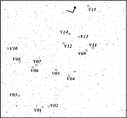
Figure 2: Finding charts for the And II variable stars. The WFC2 ($1.2\arcmin$x$1.3\arcmin$), WFC3 ($1.3\arcmin$x$1.2\arcmin$), and WFC4 ($1.2\arcmin$x$1.2\arcmin$) images are each shown in a panel. North and east directions are shown with the arrow pointing toward the north.

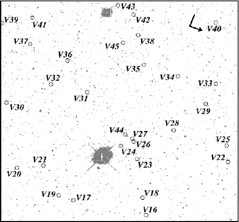
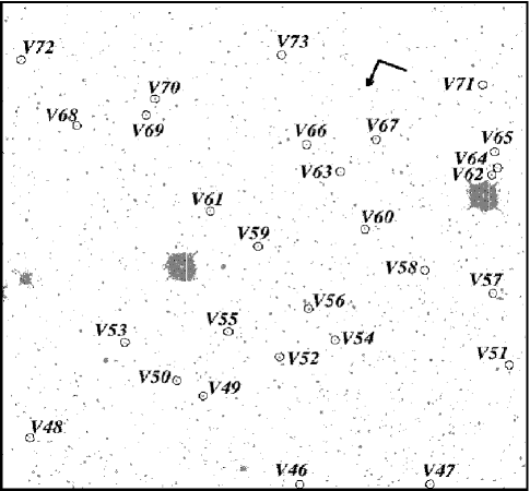
Figure 2 cont: Finding charts for the And II variable stars. The WFC2 ($1.2\arcmin$x$1.3\arcmin$), WFC3 ($1.3\arcmin$x$1.2\arcmin$), and WFC4 ($1.2\arcmin$x$1.2\arcmin$) images are each shown in a panel. North and east directions are shown with the arrow pointing toward the north.

Figure 2 cont: Finding charts for the And II variable stars. The WFC2 ($1.2\arcmin$x$1.3\arcmin$), WFC3 ($1.3\arcmin$x$1.2\arcmin$), and WFC4 ($1.2\arcmin$x$1.2\arcmin$) images are each shown in a panel. North and east directions are shown with the arrow pointing toward the north.

3 Variable Stars

As for Paper I, we searched the photometry data for variable stars using a routine created by Dr. Peter Stetson called daomaster. This routine compares the rms scatter in the magnitudes to that expected from the photometric errors returned by the allframe program. There were only a handful of RRLs found on the PC and no ACs. Because the PC covers only a small area of sky compared to the WF CCDs, and because of the lack of sufficiently bright stars for reliable aperture corrections on the PC, we do not include the PC data in our results.

Figure 1 shows the location of the variable stars in the CMD created by DACS00. We removed the DACS00 photometric data from the CMD for those stars which were found to be variable in this paper and instead plotted them as plusses representing the mean magnitude and color of the variable star. The RRLs can be seen filling in the gap in the CMD along the horizontal branch (HB). About 1.2 mag brighter than the HB is the single AC we found in this survey. The periods, magnitudes, and light curves were determined using the programs created by A. C. Layden as outlined in Paper I. We note that due to the method we have used to calibrate the data to the $B$, $V$ system, the colors and magnitudes for the variable stars have inherent uncertainties on the order of 0.02-0.03 mag. Not withstanding this fact, we find that our method allows us to analyze the general properties of the And II variable star population.

The stars that lie to the blue of the red giant branch and those DACS00 stars found within and near the instability strip on the HB in Figure 1 were examined for variability, but no additional variables were found. Two plausible explanations for the non-variability, especially for those stars found within the instability strip, are either (a) these stars are not variables, but errors in the photometry, particularly in the colors, have scattered them into an apparent location in the instability strip, or (b) these are indeed variables but the limited time coverage of the observations meant that we did not detect the variability.

DACS00 performed an initial variable star search of And II. In their paper they report detecting approximately 30 candidate variable stars. Fig. 3 of DACS00 shows the location of these variables in the And II CMD and it shows a lot of dispersion among the RRLs. As discussed in Paper I the reason for such a dispersion is that the magnitudes and colors plotted by DACS00 come from 2 pairs of combined frames which, consequently, do not correctly sample the variable star light curves. They also show light curves for four of the RRLs they detected (see Fig. 6 of DACS00). These RRLs match V57, V60, V05, and V33 in this survey, going from the top-down in their figure. The periods for V57 and V05 match well in both studies, while the periods found for V60 and V33 in this survey and DACS00 are aliases of each other. The method used in this paper to obtain the photometry for the variable stars results in having more data points than were available to DACS00 allowing a more reliable choice of the period here.

A total of 73 variable stars were found on the WFC chips, one of which is an AC. This star will be discussed in the following section. Table 2 presents the photometric properties for these variable stars while their individual photometric $B$ and $V$ data are in Tables 3 and 4. Column 1 of Table 2 lists the star’s ID, while the next two columns give the RA and Dec. Finding charts for the variable stars are shown in Figure 2. Column 4 lists the period of each star. The intensity-weighted $\langle V\rangle$ and $\langle B\rangle$ magnitudes along with the magnitude-weighted colors $(\bv)_{\rm mag}$ are shown in columns 5-7. Columns 8 and 9 give the $V$ and $B$ amplitudes of the variable stars. The remaining columns will be discussed later in the paper. In Figure 3 we present the light curves for all of the variable stars.

Figure 5: And II variable star light curves. The observations are shown as filled circles and the fitted templates are displayed as curves.

Figure 3 cont: And II variable star light curves. The observations are shown as filled circles and the fitted templates are displayed as curves.

Figure 3 cont: And II variable star light curves. The observations are shown as filled circles and the fitted templates are displayed as curves.

Figure 3 cont: And II variable star light curves. The observations are shown as filled circles and the fitted templates are displayed as curves.

4 And II Anomalous Cepheid

We were able to find one AC, V14, in the field-of-view of the WFPC2. This follows the trend of at least one AC being found in every dSph galaxy surveyed for variable stars. ACs are believed to be either stars that have increased mass due to mass transfer in a binary system (Renzini, Mengel, & Sweigart 1977) or stars from an intermediate age population (Demarque & Hirshfeld 1975; Norris & Zinn 1975) although metal-poor abundances are required in both cases. The main way to recognize ACs is by their higher luminosity when compared to the RRLs in a system, typically 0.5-2.0 mag brighter than the HB.

The ACs follow a period-luminosity relation different than that for classical Cepheids or Population II Cepheids, hence the name “anomalous.” In Paper I we revised the period-luminosity relations for the ACs (see §4.1 in Paper I). Using the data from Table 2 and given $(m-M)_{0}=24.17\pm 0.06$ and $E(\bv)=0.06\pm 0.01$ for And II from DACS00, we find $A_{V}=3.1E(\bv)=0.19\pm 0.03$ resulting in $M_{V}=-0.75$ mag and $M_{B}=-0.43$ mag for V14. This places the AC in And II with the other known ACs (see Table 4 of Paper I) in the period-luminosity diagram in Figure 4. V14 falls nicely along the first-overtone AC line in both $M_{B}$ and $M_{V}$.

We note that the light curve shape of V14 is quite asymmetric which would lead one to think it is pulsating in the fundamental mode. Yet, it is clearly a first-overtone mode pulsator as seen in Figure 4. This reinforces the view we expressed in Paper I that the shape of the light curve isn’t as clear an indicator of pulsation mode for an AC as is its location in a plot of the absolute magnitude versus the logarithm of the period. Given the $B$ and $V$ amplitudes for V14 in Table 2, this star also falls nicely among the other first-overtone mode AC pulsators in the period-amplitude diagram shown as Fig. 7 of Paper I.

Figure 9: Absolute magnitude versus period diagrams for anomalous Cepheids. Only those anomalous Cepheids with quality light curves are shown for the (a) $B$ and (b) $V$ filters. The dashed lines represent the fits to the fundamental and first-overtone anomalous Cepheids taken from Paper I. The data for the dwarf spheroidal galaxies besides And II were taken from Paper I. The And II AC V14 is shown as the filled square.

5 And II RR Lyrae

RRLs are useful when examining the stellar populations of a system. Their periods, amplitudes, and magnitudes are probes of the distance, metallicity, and age of the system in which they belong. We found 72 RRLs in our field-of-view of And II, with 64 pulsating in the fundamental mode (RRab) and eight pulsating in the first-overtone mode (RRc). Their mere presence indicates that there are stellar populations of age $>10$ Gyr in And II. Due to the low amplitudes of the RRc stars and the uncertainties in our photometry, it is likely that we did not detect all of this type of RRLs. We compare the period distribution of the RRL population of And II to those of other dSph galaxies in Figure 5 using the sources listed in Table 6 of Paper I and the values derived above for And II. The mean metallicity increases from the top, Ursa Minor, to the bottom, Fornax. It should be noted that although the mean metallicity of Fornax is $\langle{\rm[Fe/H]}\rangle=-1.3$ dex (Mateo 1998), the RRLs may originate from the metal-poor end of Fornax’s metallicity distribution (Bersier & Wood 2002). Looking at the RRab stars, there appears to be an overall trend of these stars shifting toward shorter periods as the metallicity increases. And II shows more of a spread in period among its RRab stars as compared to the other dSph galaxies. It is uncertain how much of this distribution may be due to the spread in metallicity that is known to exist in this dSph galaxy ($\sigma_{\rm int,[Fe/H]}\approx 0.36$ dex, DACS00).

The mean periods for the RRLs are $\langle P_{ab}\rangle=0.571$ day and $\langle P_{c}\rangle=0.363$ day. In comparison to the period-metallicity relationship defined by the Galactic globular clusters, the mean period for the RRab stars is consistent with the mean metallicity in And II as determined from the red giant branch. For the RRc stars, however, the mean period is slightly longer than that expected if these stars have the same mean metallicity as the red giants. As discussed above, the RRc mean period may be unreliable as it is possible we are missing many of these stars. Nevertheless, the ratio of RRc stars to the total number of RRLs, $N_{c}/N_{RR}$, is 0.11, consistent with the relatively high mean metallicity of And II. If we place And II in Table 6 of Paper I using the mean metallicity from the red giant branch, it follows the trend in which the mean period for the RRab stars decreases as the metallicity increases. To illustrate this, we reproduce the metallicity versus mean RRab period diagram of Paper I (see Fig. 10 of that paper) in Figure 6, but now include And II. With the exception of $\omega$ Centauri and M2, there is a clear trend of increasing mean period with decreasing ${\rm[Fe/H]}$ for the Galactic globular clusters. As noted in Paper I, the mean periods of the RRab stars in the dSph galaxies fill in the gap between the metal-rich and metal-poor Galactic globular clusters. And II clearly also follows this trend – it lies in Figure 6 among the Galactic globular clusters which have similar metallicities to the And II mean abundance.

Figure 10: Period distribution plots for the RR Lyrae stars in dwarf spheroidal galaxies. The plots are arranged so that the mean metallicity of the dwarf spheroidal galaxy increases from the top down. For each dwarf spheroidal galaxy, the vertical arrows indicate the mean periods for the RRc (left) and RRab (right) stars.

Figure 11: Mean period for the RRab stars versus the metallicity of the parent system. The Andromeda dwarf spheroidal galaxies are shown as open squares. The Galactic dwarf spheroidal galaxies are indicated by open circles. Galactic globular clusters with at least 15 RRab stars are shown as filled circles, along with $\omega$ Centauri (filled square). Large Magellanic Cloud globular clusters with a minimum of 15 RRab stars are shown as open triangles.

We find the mean magnitude of the And II RRLs to be $\langle V\rangle=24.87\pm 0.03$ mag, where the uncertainty is the aperture correction uncertainty, the photometry zeropoint uncertainty, and the spline-fitting uncertainty added in quadrature to the standard error of the mean. This matches the estimate of the level of the HB by DACS00, $V_{\rm HB}=24.93\pm 0.03$ mag based on the mean magnitude of the HB stars. We used the same equation as DACS00 to estimate the absolute magnitude of the RRLs,

$$M_{V,{\rm RR}}=0.17{\rm[Fe/H]}+0.82$$ (1)

from Lee, Demarque, & Zinn (1990). We find $M_{V,{\rm RR}}=+0.57$ and $A_{V}=3.1E(\bv)=0.19\pm 0.03$ given $\langle{\rm[Fe/H]}\rangle=-1.49\pm 0.11$ and $E(\bv)=0.06\pm 0.01$ from DACS00. As a result, we estimate the distance to And II to be $665\pm 20$ kpc, which matches the estimate made by DACS00 of $680\pm 20$ kpc.

5.1 RR Lyrae Period-Amplitude Diagram

The period-amplitude diagram provides an excellent diagnostic of the properties of the RRLs since neither of these quantities is dependent on distance or reddening. It is generally true that the position of RRLs in a period-amplitude diagram is dependent on its metallicity (Sandage 1993b). Still, there are other factors besides metallicity, such as evolution and age, that may shift a RRL’s position in the diagram. There is a clear division between the shorter period, smaller amplitude RRc stars and the RRab stars in the And II period-amplitude diagram (Figure 7). A wide spread in $\log\,P$ is seen among the RRab stars for a given $A_{B}$, that may or may not be due to the spread in ${\rm[Fe/H]}$ for And II (DACS00).

There may also be some aliasing in the periods. As with And VI (Paper I), we used the period-finding routines created by Dr. Andrew Layden (Layden & Sarajedini 2000 and references therein) to find the best period for each variable. We also asked Dr. Gisella Clementini to determine what periods she would find for a small number of our variable stars using her period-finding program GRATIS (GRaphical Analyzer of TIme Series, see Clementini et al. 2000, 2003). The periods she found matched those determined from Andrew Layden’s program to $\pm 0.001$ day. For And VI we were able to make use of the period-amplitude diagram to see if the period adopted for each star was reasonable. However, the red giant branch population of And II shows a large abundance dispersion which may well also occur among the RRLs. This limits the usefulness of the period-amplitude diagram in determining the most appropriate period. Therefore, we have adopted for each star the best-fit period that was returned from Layden’s period-fitting program with no further screening.

Figure 12: Period-amplitude diagram for the RR Lyrae stars in And II. The amplitudes shown are for the $B$ filter.

Sandage, Katem, & Sandage (1981) detected a shift in period between the RRLs in M3 and M15 in the period-amplitude diagram. Sandage (1981; 1982a,b) later found that this period shift was dependent on the metallicity of a cluster where metal-poor clusters tend to have longer periods for a given amplitude when compared to metal-rich clusters. Using M3 as the fiducial cluster with zero period shift, Sandage (1982a,b) found

$$\Delta\log\,P=-(0.129A_{B}+0.088+\log\,P).$$ (2)

Sandage found that more metal-rich clusters have $\langle\Delta\log\,P\rangle\geq-0.01$, while the more metal-poor clusters have $\langle\Delta\log\,P\rangle\leq-0.05$. Between these two values, a gap exists where few RRLs are found. On the other hand, as discussed in Paper I (see §5.2), dSph galaxies have been shown to contain RRLs within the $-0.05\leq\Delta\log\,P\leq-0.01$ range (Sextans: Mateo et al. 1995; Leo II: Siegel & Majewski 2000; Andromeda VI: Paper I). We list in column 10 of Table 2 the $\Delta\log\,P$ values for the RRab stars of And II. In Figure 8 we plot these values against $\log\,P$ for each RRab star. It is clear in the figure that a number of And II RRab stars are found in-between $-0.05\leq\Delta\log\,P\leq-0.01$. We find that a majority of the RRab stars are found in the metal-rich region of the diagram ($\Delta(\log\,P)>-0.01$). This is consistent with the mean metallicity of And II. When comparing And II to And VI (see Fig. 12 of Paper I), we see that there is a larger range in $\Delta\log\,P$ values in And II than in And VI. This suggests that there is a sizable abundance spread among the And II RRLs, a result that is perhaps not unexpected given the large abundance dispersion among the red giants in this dSph galaxy. The mean period shift for And II is 0.01, which means that the RRab in And II are slightly more metal-rich than M3. Using

$$\Delta\log\,P=0.116{\rm[Fe/H]}+0.173$$ (3)

from Sandage (1982a), we find ${\rm[Fe/H]}=-1.41$ for And II. This estimate of the mean metal abundance of the And II RRLs is consistent with the mean abundance for And II red giants found by DACS00, $\langle{\rm[Fe/H]}\rangle=-1.49$.

Figure 13: Period shift versus period for the RRab in And II. The dashed lines represent the zone in which few Galactic globular cluster RRab stars are found.

5.2 Metallicity Estimates from RR Lyrae

Alcock et al. (2000) developed a relation between the metallicity of a RRab star and its period and $V$-band amplitude. This was done in order to estimate the metallicity of the RRab stars in the Large Magellanic Cloud. Using the RRab stars in M3, M5, and M15, Alcock et al. found,

$${\rm[Fe/H]}_{\rm ZW}=-8.85(\log\,P_{ab}+0.15A_{V})-2.60{\rm,}$$ (4)

where ZW refers to the Zinn & West (1984) scale. The metallicity of the RRab stars in those systems was predicted with an accuracy of $\sigma_{\rm[Fe/H]}=0.31$ per star. For the LMC, Alcock et al. found good agreement between the median metallicity from their relation and those from previous estimates. We applied this relation to our And VI RRLs (see §5.3 of Paper I) and found the mean of the RRL metallicity distribution generated from this relation to agree well with the mean metallicity for the red giants determined by Armandroff, Jacoby, & Davies (1999) using the red giant branch mean $V-I$ color. The width of the metallicity distribution, however, was essentially identical to that expected from the uncertainty ($\sim 0.3$ dex) in the individual abundance determinations using this relation. Consequently, from these data, there is no evidence to support (or rule out) an abundance spread among the And VI RRLs.

Figure 14: [Fe/H] distribution plots for (a) the RRab stars in And II, (b) the RGB stars in And II from DACS00, and (c) the RRab stars in And VI from Pritzl et al. (2002). The individual [Fe/H] values for the RRab stars were calculated using Eq. 2 in Alcock et al. (2000) and have an individual uncertainty of $\sim 0.3$ dex. The abundances for the RGB stars have errors of $\sim 0.08$ dex (DACS00). Although there is no reason to expect it to be true, the distributions for the And II RRab stars and RGB stars are comparable. Their widths are much larger than that found for the And VI RRab stars ($\sigma\sim 0.3$).

We applied this equation to the RRab in And II and list the individual metallicities in column 11 in Table 2. Figure 9a shows the distribution of the individual ${\rm[Fe/H]}$ from the RRab in And II. There is a wide range among the metallicity values similar to the histogram of metallicity values derived from red giant colors for And II as found by DACS00 and shown in Figure 9b. We also plot in Figure 9c the [Fe/H] distribution from the RRab stars in And VI (Paper 1). This figure emphasizes the differences between the metallicity distributions. Where the width of the [Fe/H] distribution for the And VI RRab stars was on the order of the uncertainty of the Alcock et al. equation ($\sigma\sim 0.3$), the width for the And II stars is clearly larger than this.

Due to the wide spread in the metallicities, we did not attempt to fit a gaussian to the distribution as was done for And VI in Paper I. However, we find the mean to be ${\rm[Fe/H]}=-1.46$ and the median to be ${\rm[Fe/H]}=-1.36$. These both agree well with the mean metallicity found by DACS00 using the colors of the red giant branch stars, $\langle{\rm[Fe/H]}\rangle=-1.49\pm 0.11$. It appears that the mean metallicity values resulting from RRLs and red giants in And II are consistent. Even though the metallicity distributions for the RGB and RRab stars are comparable, there is no reason why one should expect this. The mapping from the RGB to the instability strip is a complex function of (at least) metallicity, age distributions, and evolution within the instability strip as well as whatever parameters control mass-loss. Most And II RGB stars do not become a RRL, which is clear from looking at the stellar distribution along the HB. Nevertheless, it is intriguing that the range of abundances from the RGB and RRab stars is similar and they both show a peak in the distribution near the metal-rich end.

Studying cluster and field RRLs with a wide range of metallicities, Sandage (1993a) related the metallicities to the average periods of RRLs through the relations

$${\rm[Fe/H]}_{\rm ZW}=(-\log\,\langle\,P_{ab}\rangle-0.389)/0.092$$ (5)

$${\rm[Fe/H]}_{\rm ZW}=(-\log\,\langle\,P_{c}\rangle-0.670)/0.119{\rm.}$$ (6)

Siegel & Majewski (2000) and Cseresnjes (2001) found that these relations applied well to the RRLs in dSph galaxies. We found in Paper I that the RRab estimate for And VI was within the combined errors of the estimate and that of Armandroff, Jacoby, & Davies (1999). The RRc abundance estimate, however, was lower than expected from the RRab and red giant branch stars, perhaps as a consequence of incompleteness in the sample of RRc stars, especially at shorter periods. The mean periods for the RRLs in And II are $\langle P_{ab}\rangle=0.571\pm 0.005$ day and $\langle P_{c}\rangle=0.363\pm 0.005$ day giving ${\rm[Fe/H]}_{\rm ZW}=-1.58\pm 0.04$ (internal error) for the RRab and ${\rm[Fe/H]}_{\rm ZW}=-1.93\pm 0.05$ (internal error) for the RRc. The metallicity estimate from the RRab stars, although slightly lower than the estimate made by DACS00, is within the combined errors. Once again, however, the estimate from the RRc stars is lower than that for the RRab and the red giant branch stars. It is possible that we have not detected all the RRc stars, especially at shorter periods, resulting in an inappropriate mean period (see §5).

6 The Frequency of Anomalous Cepheids in dSph Galaxies

Mateo, Fischer, & Krzeminski (1995) examined the specific frequency of ACs (the number of ACs per $10^{5}L_{V,\odot}$) in the Galactic dSph galaxies and found a strong correlation between the specific frequency of ACs and the total luminosities of the parent galaxies: low luminosity dSph galaxies have higher specific frequencies of ACs. Interpretation of this correlation, however, is complicated. For example, Draco, Ursa Minor, and Carina all have similar luminosities and similar AC specific frequencies, but they have very different stellar populations. Draco and Ursa Minor are dominated by old stars and thus, in these particular dSphs, the ACs must have their origin in the binary mass transfer mechanism. On the other hand, Carina has a strong intermediate-age population and consequently, at least some of the ACs in this dSph may originate as single younger stars, rather than from (old) mass transfer binaries. Given these differences, there is no obvious reason why Carina should end up with a similar specific frequency to Draco and Ursa Minor. Similarly, Leo I has a dominant and relatively young intermediate-age metal-poor population (Gallart et al. 1999), yet its specific frequency of ACs is notably lower than that of Draco, Ursa Minor and Carina. Mateo et al. (1995) noted that dSph luminosities are strongly correlated with mean abundance (lower abundances for lower luminosities) and that this might be the underlying cause of the AC specific frequency - luminosity correlation: regardless of the origin of the ACs, they occur more frequently in metal-poorer environments.

Figure 15: Specific frequency of anomalous Cepheids in dwarf spheroidal galaxies as a function of (a) the $M_{V}$ and (b) the mean [Fe/H] of the galaxy. The Galactic dwarf spheroidal galaxies are shown as open circles and the M31 ones are shown as filled circles. In both plots, there are clear trends that the Galactic dwarf spheroidal galaxies follow as shown by the least squares fit lines fit to their data. Both And II and And VI follow these trends.

There are now several more surveys for variable stars in dSph galaxies, including our surveys of the M31 dSph galaxies, than were available to Mateo et al. (1995). This may help disentangle the independent parameter(s) that drive the AC frequencies. In Table 5, we present revised values for Mateo et al. Table 7; we include the results from the latest surveys. For example, Dall’Ora et al. (2003) have identified 15 ACs in Carina, almost twice as many as previously known. In Table 5, Column 1 lists the dSph galaxy and column 2 is the mean [Fe/H]. The absolute magnitude of the galaxy is in column 3, and the structural parameters for each galaxy are given in columns 4–6 as the position angle measured from the North to the East, the ratio of the semi-minor axis to the semi-major axis, and the exponential scale length. The latter parameters are taken from the references given in the notes to the table. The percentage of the dSph luminosity surveyed and the number of ACs found are listed in columns 7 and 8, respectively. The specific frequencies of the ACs are then given in column 9, along with the logarithms of the specific frequencies and their uncertainties in column 10. $S$ is defined as the number of ACs per $10^{5}L_{V,\odot}$ and was calculated for only the fraction of the dSph’s luminosity that was surveyed for variable stars. The uncertainties in the $\log\,S$ values were determined by assuming that the number of observed ACs is subject to Poisson statistics.

In order to calculate the luminosity surveyed in And VI and And II, we first determined the orientation and location of the region covered by the WFPC2 images relative to the galaxy. We then calculated the intensity of the WFPC2 overlap region relative to the entire galaxy by approximating the surface brightness distribution of the galaxy by the relation $I=I_{0}e^{-(r/r_{0})^{n}}$ (Sersic 1968), and making the appropriate allowance for the ellipticities. The $V$-band surface brightness profile parameters were taken from Caldwell et al. (1992) for And II and from Caldwell (1999) for And VI. From the luminosity fractions just calculated and the total visual magnitudes of the galaxies (column 3 of Table 5) we then derive the ($V$-band) luminosity encompassed by our images of each galaxy to which the AC surveys apply. The same process was applied for the Fornax dSph galaxy according to the survey area of the Bersier & Wood (2002) survey.

Using the data from Table 5, the logarithm of the specific frequency of ACs is plotted against $M_{V}$ for each galaxy in Fig. 10a, while in Fig. 10b, the logarithm of the specific frequency is plotted against the mean [Fe/H] for each dwarf. The Galactic dSph galaxies are shown as open circles and the M31 dSph galaxies as filled circles. In each plot the solid line is an unweighted least squares fit to the Galactic dSph data only. We confirm in Fig. 10a that a $\log\,S$ – (visual) luminosity correlation exists (correlation coefficient is 0.86) for the Galactic dSph galaxies. The correlation between $\log\,S$ and mean abundance shown in Fig. 10b is not as strong (correlation coefficient 0.74) but it is nevertheless significant – a correlation test shows that there is only a 4% probability (2.3-sigma) that the distribution of $\log\,S$ vs [Fe/H] arises by chance. This supports the contention of Mateo et al. (1995) that the mean abundance of dSph galaxies may be the underlying factor that governs the frequency of occurrence of AC variables, at least for the Galactic dSphs.

The addition of data for the M31 dSphs then allows us to investigate, at least in a preliminary way, whether these correlations apply also to the AC populations in dSph galaxies other than those of the Galaxy. The points for And II and And VI in Figs. 10a and 10b, indicate that these galaxies do appear to follow the relations as defined by the Galactic dSphs, but results for additional M31 dSphs are required to strengthen this conclusion. We will return to this question in our third paper in this series, where we will explore the variable star population, including ACs, of the M31 companions And I and And III.

7 Summary & Conclusions

Although it is one of the more metal-rich dSph galaxies, the properties of the variable stars in And II agree well with the trends defined by other dSph galaxies. We have found 73 variable stars in And II using HST/WFPC2 observations, one of which is an AC. The AC is found to have a period, absolute magnitude, and amplitude consistent with other ACs. The 72 RRLs were made up of 64 RRab stars and 8 RRc stars with mean periods of $\langle P_{ab}\rangle=0.571\pm 0.005$ day and $\langle P_{c}\rangle=0.382\pm 0.005$ day. The mean $V$ magnitude of the RRLs was found to be $24.87\pm 0.03$ mag resulting in a distance of $665\pm 20$ kpc for And II on the Lee, Demarque, & Zinn (1990) distance scale.

Using relations from Sandage (1982a, 1993a) and Alcock et al. (2000), we find that the properties of the RRab stars in And II yield estimates of the mean abundance of these stars that are in good agreement with the mean metallicity determined from both the colors (DACS00) and the line strengths (Côté et al. 1999) of And II’s red giants. With these results And II then follows the general trend seen in the Galactic globular clusters and Galactic dSphs in which the mean RRab period decreases with increasing metallicity. In addition, the And II RRLs show considerable spread in the period-amplitude diagram. We take this as an indication that there is a sizable abundance spread among these stars and have attempted to quantify this spread through use of the Alcock et al. (2000) relation. This yields an abundance distribution for the RRL which is considerably broader than that expected from the errors in the individual abundance determinations and contrasts with the case for And VI (Paper I) where there was no evidence for any intrinsic abundance spread among the RRL stars. The And II RRL abundance distribution is approximately uniform and has some features in common with the large metallicity spread derived by Côté et al. (1999) and DACS00 for the red giant branch stars (see Fig. 9).

We have investigated the existence of a relationship between the specific frequency of ACs and mean metallicities for dSph galaxies. As originally suggested by Mateo et al. (1995), we find for the Galactic dSphs there is a clear trend for higher specific frequencies at lower abundances. The M31 dSph galaxies And II and And VI also appear to follow this trend. However, more information on the frequency of occurrence of ACs in additional M31 dSph galaxies is required before we can fully compare the two sets of dSphs in this parameter plane.

Table 1: Photometric Differences

Chip	$\Delta V$	# $V$ Stars	$\Delta B$	# $B$ Stars
	$21.5<V<25.5$		$23.0<B<26.0$
WFC2	–0.050 $\pm$ 0.002	302	–0.100 $\pm$ 0.003	261
WFC3	–0.076 $\pm$ 0.002	487	–0.094 $\pm$ 0.003	435
WFC4	–0.070 $\pm$ 0.002	405	–0.062 $\pm$ 0.003	360

Note. — difference = magnitude in present study – Da Costa et al. (2000) magnitude

Table 2: Light Curve Properties

ID	RA (2000)	Dec (2000)	Period	$\langle V\rangle$	$\langle B\rangle$	$(B-V)_{\rm mag}$	$A_{V}$	$A_{B}$	$\Delta\log\,P$	[Fe/H]	Classification
(1)	(2)	(3)	(4)	(5)	(6)	(7)	(8)	(9)	(10)	(11)	(12)
V01	1:16:20.49	33:26:11.8	0.407	24.808	25.211	0.410	0.35	0.50	$\cdots$	$\cdots$	c
V02	1:16:20.25	33:26:13.4	0.546	24.963	25.343	0.396	0.62	0.88	0.06	-1.10	ab
V03	1:16:21.73	33:26:13.9	0.520	24.800	25.178	0.412	0.83	1.18	0.04	-1.19	ab
V04	1:16:19.88	33:26:35.6	0.540	24.812	25.144	0.350	0.64	0.90	0.06	-1.08	ab
V05	1:16:20.52	33:26:37.0	0.583	24.926	25.274	0.403	1.06	1.50	-0.05	-1.93	ab
V06	1:16:21.61	33:26:34.0	0.590	24.870	25.267	0.447	1.08	1.52	-0.05	-2.01	ab
V07	1:16:21.48	33:26:36.1	0.481	24.781	25.154	0.408	0.83	1.17	0.08	-0.89	ab
V08	1:16:22.27	33:26:34.6	0.552	24.812	25.246	0.477	1.02	1.43	-0.01	-1.67	ab
V09	1:16:19.54	33:26:54.4	0.547	24.939	25.401	0.468	0.37	0.53	0.11	-0.77	ab
V10	1:16:23.03	33:26:40.6	0.605	24.870	25.288	0.444	0.73	1.03	0.00	-1.64	ab
V11	1:16:19.30	33:26:57.1	0.778	24.929	25.412	0.496	0.58	0.81	-0.08	-2.41	ab
V12	1:16:20.68	33:26:54.4	0.514	24.901	25.370	0.504	0.92	1.30	0.03	-1.26	ab
V13	1:16:20.11	33:27:01.4	0.544	24.855	25.271	0.453	0.85	1.20	0.02	-1.39	ab
V14	1:16:20.57	33:27:01.5	0.578	23.608	23.990	0.419	0.91	1.29	$\cdots$	$\cdots$	AC
V15	1:16:20.21	33:27:21.7	0.470	24.889	25.311	0.463	0.99	1.39	0.06	-1.01	ab
V16	1:16:23.80	33:26:38.1	0.346	24.848	25.086	0.248	0.42	0.59	$\cdots$	$\cdots$	c
V17	1:16:23.55	33:26:14.9	0.575	24.944	25.371	0.456	0.82	1.16	0.00	-1.57	ab
V18	1:16:24.20	33:26:35.1	0.700	24.933	25.201	0.285	0.59	0.84	-0.04	-2.01	ab
V19	1:16:23.55	33:26:10.0	0.489	24.800	25.096	0.372	1.24	1.75	0.00	-1.50	ab
V20	1:16:23.88	33:25:54.6	0.508	24.941	25.276	0.371	0.92	1.31	0.04	-1.22	ab
V21	1:16:24.16	33:26:02.1	0.456	24.821	25.156	0.373	0.95	1.34	0.08	-0.84	ab
V22	1:16:25.81	33:26:56.4	0.398	24.850	25.133	0.293	0.43	0.61	$\cdots$	$\cdots$	c
V23	1:16:25.12	33:26:29.2	0.540	24.845	25.177	0.347	0.58	0.82	0.07	-1.00	ab
V24	1:16:25.30	33:26:22.9	0.697	24.857	25.283	0.458	0.86	1.21	-0.09	-2.35	ab
V25	1:16:26.21	33:26:54.2	0.519	25.021	25.426	0.464	1.17	1.65	-0.02	-1.63	ab
V26	1:16:25.52	33:26:26.2	0.696	24.862	25.228	0.376	0.47	0.66	-0.02	-1.83	ab
V27	1:16:25.59	33:26:25.5	0.509	24.868	25.216	0.381	0.89	1.25	0.04	-1.19	ab
V28	1:16:26.14	33:26:36.9	0.549	24.796	25.239	0.458	0.58	0.81	0.07	-1.07	ab
V29	1:16:27.08	33:26:43.4	0.385	24.914	25.163	0.261	0.47	0.67	$\cdots$	$\cdots$	c
V30	1:16:25.41	33:25:44.1	0.545	24.861	25.308	0.462	0.55	0.78	0.07	-1.00	ab
V31	1:16:26.36	33:26:06.9	0.505	24.915	25.270	0.369	0.51	0.73	0.11	-0.65	ab
V32	1:16:26.25	33:25:55.3	0.651	24.824	25.248	0.429	0.36	0.51	0.03	-1.43	ab
V33	1:16:27.66	33:26:44.2	0.517	24.872	25.316	0.463	0.63	0.88	0.08	-0.90	ab
V34	1:16:27.53	33:26:32.0	0.449	24.744	25.023	0.334	1.13	1.60	0.05	-1.02	ab
V35	1:16:27.52	33:26:20.7	0.483	24.794	25.068	0.324	1.07	1.52	0.03	-1.22	ab
V36	1:16:26.98	33:25:57.5	0.538	25.085	25.392	0.329	0.66	0.93	0.06	-1.09	ab
V37	1:16:27.07	33:25:44.7	0.751	25.017	25.271	0.266	0.51	0.72	-0.06	-2.18	ab
V38	1:16:28.21	33:26:15.7	0.695	24.897	25.301	0.441	0.94	1.33	-0.10	-2.45	ab
V39	1:16:27.35	33:25:34.2	0.509	24.902	25.126	0.292	1.13	1.61	0.00	-1.50	ab
V40	1:16:29.17	33:26:37.2	0.665	24.895	25.235	0.364	0.74	1.04	-0.04	-2.01	ab
V41	1:16:27.73	33:25:42.4	0.566	24.897	25.253	0.405	1.07	1.51	-0.04	-1.83	ab
V42	1:16:28.68	33:26:12.0	0.341	24.780	25.214	0.454	0.59	0.83	$\cdots$	$\cdots$	c
V43	1:16:28.77	33:26:06.3	0.490	24.931	25.280	0.379	0.85	1.19	0.07	-0.99	ab
V44	1:16:25.63	33:26:23.0	0.572	24.829	25.271	0.452	0.47	0.66	0.07	-1.08	ab
V45	1:16:27.89	33:26:12.1	0.797	24.842	25.310	0.473	0.34	0.48	-0.05	-2.18	ab
V46	1:16:25.41	33:25:37.8	0.620	24.833	25.203	0.414	0.95	1.34	-0.05	-2.02	ab
V47	1:16:26.77	33:25:31.4	0.763	24.807	25.140	0.379	1.01	1.43	-0.09	-2.32	ab
V48	1:16:22.39	33:25:44.2	0.736	24.873	25.335	0.483	0.65	0.92	-0.07	-2.28	ab
V49	1:16:24.02	33:25:30.0	0.544	24.919	25.314	0.409	0.54	0.77	0.08	-0.98	ab
V50	1:16:23.68	33:25:29.1	0.575	24.708	25.112	0.420	0.64	0.90	0.04	-1.32	ab
V51	1:16:27.10	33:25:10.7	0.673	24.706	25.093	0.422	0.91	1.29	-0.08	-2.29	ab
V52	1:16:24.66	33:25:20.8	0.472	24.810	25.181	0.399	0.75	1.07	0.10	-0.71	ab
V53	1:16:22.98	33:25:26.2	0.316	24.861	25.246	0.398	0.47	0.66	$\cdots$	$\cdots$	c
V54	1:16:25.18	33:25:15.7	0.454	24.916	25.263	0.380	0.88	1.24	0.09	-0.73	ab
V55	1:16:24.02	33:25:19.7	0.595	24.833	25.151	0.355	0.85	1.20	-0.02	-1.73	ab
V56	1:16:24.77	33:25:12.5	0.604	24.921	25.333	0.446	0.90	1.27	-0.03	-1.86	ab
V57	1:16:26.63	33:25:01.4	0.496	24.944	25.238	0.351	1.15	1.63	0.01	-1.43	ab
V58	1:16:25.83	33:25:01.4	0.282	24.839	25.232	0.403	0.41	0.58	$\cdots$	$\cdots$	c
V59	1:16:23.98	33:25:06.1	0.557	24.830	25.178	0.355	0.42	0.59	0.09	-0.91	ab
V60	1:16:25.03	33:24:58.4	0.560	24.912	25.182	0.322	1.08	1.53	-0.03	-1.81	ab
V61	1:16:23.33	33:25:03.4	0.442	24.871	25.200	0.372	0.92	1.30	0.10	-0.68	ab
V62	1:16:26.12	33:24:44.7	0.466	24.886	25.143	0.310	1.11	1.57	0.04	-1.14	ab
V63	1:16:24.53	33:24:51.5	0.502	24.797	25.038	0.289	1.05	1.48	0.02	-1.33	ab
V64	1:16:26.15	33:24:43.5	0.530	24.823	25.178	0.423	1.17	1.65	-0.03	-1.71	ab
V65	1:16:26.06	33:24:41.3	0.686	24.907	25.244	0.384	0.95	1.35	-0.10	-2.41	ab
V66	1:16:24.06	33:24:49.3	0.467	24.883	25.219	0.378	0.94	1.34	0.07	-0.92	ab
V67	1:16:24.77	33:24:45.2	0.466	24.900	25.231	0.386	1.06	1.50	0.05	-1.07	ab
V68	1:16:21.58	33:24:57.8	0.736	24.824	25.240	0.423	0.41	0.58	-0.03	-1.97	ab
V69	1:16:22.26	33:24:52.9	0.430	24.737	25.128	0.404	0.48	0.67	$\cdots$	$\cdots$	c
V70	1:16:22.28	33:24:50.2	0.707	25.011	25.474	0.475	0.52	0.73	-0.03	-1.96	ab
V71	1:16:25.65	33:24:32.5	0.474	24.958	25.358	0.421	0.70	0.99	0.11	-0.66	ab
V72	1:16:20.70	33:24:50.3	0.469	24.841	25.190	0.390	0.99	1.40	0.06	-1.00	ab
V73	1:16:23.43	33:24:37.9	0.698	24.761	25.128	0.432	1.12	1.58	-0.08	-2.19	ab

Table 3: Photometry of the Variable Stars ($B$)

	V01			V02
HJD-2450000	$B$	$\sigma_{B}$		$B$	$\sigma_{B}$
690.268	25.118	0.156		$\cdots$	$\cdots$
690.319	25.254	0.117		24.594	0.107
690.336	25.285	0.164		0.000	0.000
690.386	25.288	0.139		24.867	0.108
690.403	$\cdots$	$\cdots$		25.020	0.108
690.454	24.921	0.080		25.183	0.119
690.471	24.930	0.124		25.171	0.108
695.226	25.348	0.131		24.916	0.103
695.242	25.519	0.154		24.835	0.087
695.293	25.156	0.061		$\cdots$	$\cdots$
695.310	25.090	0.106		25.007	0.182
695.360	24.828	0.127		25.198	0.214
695.377	$\cdots$	$\cdots$		25.284	0.137
695.385	24.880	0.121		25.325	0.115
695.444	24.963	0.144		25.267	0.140

Note. — The complete version of this table is in the electronic edition of the Journal. The printed edition contains only a sample.

Table 4: Photometry of the Variable Stars ($V$)

	V01			V02
HJD-2450000	$V$	$\sigma_{V}$		$V$	$\sigma_{V}$
690.185	24.712	0.164		25.147	0.171
690.201	24.779	0.061		25.202	0.106
690.251	$\cdots$	$\cdots$		25.085	0.090
695.092	$\cdots$	$\cdots$		25.109	0.118
695.108	$\cdots$	$\cdots$		25.019	0.119
695.158	24.894	0.097		25.194	0.097
695.174	24.956	0.091		24.983	0.074

Note. — The complete version of this table is in the electronic edition of the Journal. The printed edition contains only a sample.

Table 5: Frequency of Anomalous Cepheids in Dwarf Spheroidal Galaxies

Galaxy	$\langle{\rm[Fe/H]}\rangle$	$M_{V}$	PA	$1-b/a$	$r_{\rm exp}$	Surveyed L	$N_{\rm AC}$	$S$	$\log\,S$	References
			(degrees)		(arcmin)	(%)
Ursa Minor	–2.2	–8.9	53	0.55	5.8	90	6	2.3	$0.36^{+0.15}_{-0.23}$	1,2,3,14
Carina	–2.0	–8.9	65	0.33	5.5	100	15	4.8	$0.68^{+0.10}_{-0.13}$	1,2,15,18
Draco	–2.0	–8.9	82	0.29	4.5	55	5	3.8	$0.58^{+0.16}_{-0.26}$	1,2,13
Leo II	–1.9	–10.2	12	0.13	1.5	100	4	0.40	$-0.40^{+0.18}_{-0.30}$	1,2,12
Sculptor	–1.8	–10.7	99	0.34	6.5	55	3	0.35	$-0.46^{+0.20}_{-0.36}$	1,2,3,16
Sextans	–1.7	–10.0	56	0.40	9.1	75	6	1.0	$0.00^{+0.18}_{-0.30}$	1,2,3
Leo I	–1.7	–11.7	79	0.30	1.6	100	12	0.30	$-0.52^{+0.11}_{-0.16}$	1,2,3,5,11
Fornax	–1.3	–13.7	48	0.30	10.5	34	18	0.22	$-0.66^{+0.09}_{-0.11}$	1,3,8,9,10
And VI	–1.6	–11.3	160	0.23	1.4	21	6	1.1	$0.04^{+0.14}_{-0.24}$	4,6,7,8
And II	–1.5	–11.7	155	0.30	1.6	18	1	0.14	$-0.85^{+0.31}_{-inf}$	3,8,17

Note. — PA is the position angle measured from the North to the East. References: (1) Mateo (1998); (2) Mateo et al. (1995); (3) Caldwell et al. (1992); (4) Caldwell (1999); (5) Gallart et al. (1999); (6) Armandroff et al. (1999); (7) Pritzl et al. (2002); (8) This paper; (9) Bersier & Wood (2002); (10) Light et al. (1986); (11) Hodge & Wright (1978); (12) Siegel & Majewski (2000); (13) Baade & Swope (1961); (14) Nemec et al. (1988); (15) Saha et al. (1986); (16) Kaluzny et al. (1995); (17) Da Costa et al. (2000); (18) Dall’Ora et al. (2003)

References

- Alcock et al. (2000) Alcock, C., et al. 2000, AJ, 119, 2194
- Armandroff, Jacoby, & Davies (1999) Armandroff, T. E., Jacoby, G. H., & Davies, J. E. 1999, AJ, 118, 1220
- Baade & Swope (1961) Baade, W., & Swope, H. H. 1961, AJ, 66, 300
- Bersier & Wood (2002) Bersier, D., & Wood, P. R. 2002, AJ, 123, 840
- Caldwell (1999) Caldwell, N. 1999, AJ, 118, 1230
- Caldwell et al. (1992) Caldwell, N., Armandroff, T. E., Seitzer, P., & Da Costa, G. S. 1992, AJ, 103, 840
- Clementini et al. (2000) Clementini, G., et al. 2000, AJ, 120, 2054
- Clementini et al. (2003) Clementini, G., Gratton, R., Bragaglia, A., Carretta, E., Di Fabrizio, L., & Marcella, M. 2003, AJ, 125, 1309
- Côté, Oke, & Cohen (1999) Côté, P., Oke, J. B., & Cohen, J. G. 1999, AJ, 118, 1645
- Cseresnjes (2001) Cseresnjes, P. 2001, A&A, 375, 909
- Da Costa et al. (2000) Da Costa, G. S., Armandroff, T. E., Caldwell, N., & Seitzer, P. 2000, AJ, 119, 705 (DACS00)
- Dall’Ora et al. (2003) Dall’Ora, M., et al. 2003, AJ, 126, 197
- Demarque & Hirshfeld (1975) Demarque, P., & Hirshfeld, A. W. 1975, ApJ, 202, 346
- Gallart et al. (1999) Gallart, C., Freedman, W. L., Aparicio, A., Bertelli, G., & Chiosi, C. 1999, AJ, 118, 2245
- Hodge & Wright (1978) Hodge, P. W., & Wright, F. W. 1978, AJ, 83, 228
- Ibata, Gilmore, & Irwin (1994) Ibata, R. A., Gilmore, G., & Irwin, M. J. 1994, Nature, 370, 194
- Kaluzny et al. (1995) Kaluzny, J., Kubiak, M., Szymanski, M., Udalski, A., Krzeminski, W., & Mateo, M. 1995, A&AS, 112, 407
- Layden & Sarajedini (2000) Layden, A. C., & Sarajedini, A. 2000, AJ, 119, 1760
- Lee, Demarque, & Zinn (1990) Lee, Y. W., Demarque, P., & Zinn, R. 1990, ApJ, 350, 155
- Light, Armandroff, & Zinn (1986) Light, R. M., Armandroff, T. E., & Zinn, R. 1986, AJ, 92, 43
- Mateo (1998) Mateo, M. 1998, ARA&A, 36, 435