Morphology of Rising Hydrodynamic and Magneto-hydrodynamic Bubbles from Numerical Simulations

Abstract

Recent Chandra and XMM-Newton observations of galaxy cluster cooling flows have revealed X-ray emission voids of up to 30 kpc in size that have been identified with buoyant, magnetized bubbles. Motivated by these observations, we have investigated the behavior of rising bubbles in stratified atmospheres using the Flash adaptive-mesh simulation code. We present results from 2-D simulations with and without the effects of magnetic fields, and with varying bubble sizes and background stratifications. We find purely hydrodynamic bubbles to be unstable; a dynamically important magnetic field is required to maintain a bubble’s integrity. This suggests that, even absent thermal conduction, for bubbles to be persistent enough to be regularly observed, they must be supported in large part by magnetic fields. Thermal conduction unmitigated by magnetic fields can dissipate the bubbles even faster. We also observe that the bubbles leave a tail as they rise; the structure of these tails can indicate the history of the dynamics of the rising bubble.

1 INTRODUCTION

Cooling flows have been known for some time to exist at the centers of some clusters of galaxies (see Fabian 1994 for a review). The X-ray emissivity of the intracluster medium (ICM) increases with the square of the plasma density, and as the ICM is very centrally concentrated, radiative energy losses are greatest at the center of a cluster. In rich clusters these losses over the life of the cluster can be significant enough, in the absence of thermal conduction, to cause the plasma to contract gradually within the cluster potential and flow inward with velocities of order a few tens of km s^-1. It has been understood that — again, in the absence of conduction – the cooling gas must become thermally unstable to the formation of a multiphase medium below about 0.1 $\mathrm{keV}$, but the fate of this cold gas – as stars, cold X-ray-absorbing clouds, or even brown dwarfs – has been a mystery. The possibility that some energetic feedback mechanism could shut off the cooling flows has been subject to debate, as well as the role played by thermal conduction and magnetic fields.

Recent high-resolution X-ray observations by the Chandra and XMM-Newton satellites have dramatically changed this picture (Böhringer et al., 2002). First, no evidence from spatially resolved spectroscopy has been observed for the presence of gas colder than about 1–2 $\mathrm{keV}$ (e.g., Schmidt et al. 2001; Peterson et al. 2001; Kaastra et al. 2001; Tamura et al. 2001; Matsushita et al. 2002). Second, high-resolution imaging has provided evidence for large-scale motions that can heat the ICM (e.g., McNamara et al. 2000; McNamara et al. 2001; Forman et al. 2002; Blanton et al. 2003). For years it has been known that many of the same clusters that harbor cooling flows also contain large central galaxies with active nuclei. However, the extent to which these active galactic nuclei (AGN) influence the dynamical state of the cooling ICM has only become apparent through the new X-ray observations. These observations show that AGN produce massive outflows of magnetized plasma that displace the cooling gas. The ‘bubbles’ thus produced are known to be magnetized because radio observations show regions of synchrotron emission coinciding with the regions of low X-ray emission, and the polarization of this radiation shows Faraday rotation effects consistent with dynamically important magnetic fields (e.g., Allen et al. 2001; Nulsen et al. 2002). The emerging picture is that bubbles represent the late stages of propagation of the magnetized, relativistic jets produced by AGN into the ICM, after they have slowed and reached approximate pressure equilibrium with the ICM (Reynolds et al., 2002).

The influence of these magnetized bubbles on the cooling ICM is still poorly understood. How efficiently does the bubble plasma mix with the ICM? Does it heat the cooling flow sufficiently to avoid the formation of multiphase gas and the possible formation of stars? If so, how – by radiative heating, magnetic reconnection, or some other process? What fraction of the total energy budget of a cluster is contributed by magnetic fields and cosmic rays? Could these active regions be sites for the acceleration of the ultra-high-energy cosmic rays seen in some air-shower experiments?

Owing to the geometrical and physical complexity of the AGN-cooling flow environment, numerical simulations are the best theoretical tools available for addressing these questions. While bubbles in liquids are well-studied (see, e.g., Magnaudet and Eames 2000; Harper 1972), bubbles in cluster cooling flows should differ from bubbles in liquids in several important ways. In particular, molecular forces present in liquids (e.g., surface tension, viscosity) will not play a significant role, and magnetic fields may be important. These differences will affect the dynamics and stability properties of bubbles.

Several numerical studies have been performed recently of rising bubbles in the context of cluster cooling flows. Churazov et al. (2001) used 2-D hydrodynamic simulations in a cooling-flow model atmosphere to gain insight into the bubbles observed in M87. Brüggen and Kaiser (2002, 2001) studied 2-D spherical and elliptical magnetohydrodynamic (MHD) bubbles rising in a hydrostatic background medium with an isothermal $\beta$-model density profile (Cavaliere and Fusco-Femiano, 1976),

$$\rho(r)\propto[1+(r/r_{c})^{2}]^{-3\beta/2}\ ,$$ (1)

where $r_{c}\sim 200$ $\mathrm{keV}$ is the core radius and $\beta$ was taken to be 0.5. Brüggen et al. (2002) performed 3-D hydrodynamic bubble simulations with continuous energy injection. More recently, Basson and Alexander (2003) have performed 3-D hydrodynamic simulations of both the active and inactive phases of AGN jets propagating into $\beta$-model density profiles, including radiative cooling. In addition, several papers have addressed the detectability in radio and X-rays of cluster bubbles, including Churazov et al. (2001), Brüggen and Kaiser (2001), Ensslin and Heinz (2002), and Soker et al. (2002). Finally, bubbles in stratified atmospheres have been studied in the context of contact binary stars by Brandenburg and Hazlehurst (2001).

In this paper, we study the general question of the behavior of a buoyant gas bubble rising in a denser gas, investigating the relative importance of the effects of geometry, stratification, density contrast, and thermal and magnetic pressure on the stability of the bubble. Most of the previous studies (both 2-D and 3-D) have used finite-difference methods to evolve the gas on relatively low-resolution grids, up to about 400 zones on a side. Brüggen (2003) and Brüggen and Kaiser (2002) used the Flash code (Fryxell et al., 2000), which has an adaptive mesh (MacNeice et al., 2000) to achieve an effective resolution of 4,000$\times$2,000 zones for purely hydrodynamic calculations. We also employ Flash, but in addition to hydrodynamic bubbles we study the effects of magnetic fields with different spatial configurations, exploiting a new MHD module we have developed for Flash. In addition, because we do not treat the bubbles as self-gravitating, we are able to use for the hydrodynamic case a version of the piecewise parabolic method (PPM) that has been modified to handle nearly hydrostatic flows (Zingale et al., 2002). Our initial model is deliberately simplified as a first step in a research program to better understand the dynamics of bubbles in clusters; thus we postpone detailed observational comparisons to a later paper.

The paper is organized as follows: in § 2 we describe the construction of our initial models and the numerical methods used. In § 3 we discuss the results of our purely hydrodynamic calculations. In § 4 we discuss results of simulations of hot bubbles rising in background magnetic fields, and in § 5 we consider magnetized bubbles initially supported partly by force-free magnetic fields. In § 6 we summarize our conclusions.

2 INITIAL MODELS

We consider as initial models an under-dense circular bubble in an isothermal, stratified atmosphere with an imposed constant gravitational acceleration in the $y$-direction. An ideal equation of state is used, with a ratio of specific heats $\gamma=5/3$. The sound speed was chosen, through the temperature and mean molecular weight, so that our standard simulation domain would span approximately three pressure scale heights. For most of our simulations, we simulate 2-D boxes in planar geometry. We vary the stratification by varying the gravitational acceleration. We also vary the size of the bubble.

We perform simulations in which the density contrast between the bubble and the background is caused by a higher temperature in the bubble in horizontal pressure equilibrium with its surroundings (the ‘hot bubble’ case) and also in which the pressure support for the under-dense bubble comes from an azimuthal magnetic field (the ‘magnetized bubble’ case). In the ‘hot bubble’ case, we perform simulations with and without a background magnetic field. The bubble is in horizontal pressure equilibrium at every point inside the bubble; since the bubbles considered here are significant fractions of a pressure scale height, the bubble’s pressure structure is itself somewhat stratified.

The physics in the simulations presented is all scale-free. For numerical reasons, we choose scales for the simulations so that numbers simulated are all near unity. Thus, our simulations were performed with a domain size of $40\times 50$ cm, and the bubble radius of $3$ cm. The base density and pressure are taken to be of order unity ($\rho_{0}=1$, $p_{0}\approx.64$) and gravitational acceleration is $0.04~{}\mathrm{cm\ s^{-2}}$. For comparison to the astrophysical systems of interest, however, we rescale the results when plotting figures. We rescale by scaling the length scales by a factor $L$, the gravitational acceleration by $G$, and the density by $R$. In that case, the hydrodynamic quantities scale as

$$x = Lx^{\prime}$$ (2)

$$t = \sqrt{\frac{L}{G}}t^{\prime}$$ (3)

$$v = \sqrt{LG}v^{\prime}$$ (4)

$$g = Gg^{\prime}$$ (5)

$$\rho = R\rho^{\prime}$$ (6)

$$p = \left(RGL\right)p^{\prime},$$ (7)

where the primed quantities represent the simulated values, and unprimed represent the scaled values. Here, $x$ is a length, $t$ time, $v$ velocity, $g$ the gravitational acceleration, $\rho$ density, and $p$ pressure. The values presented here are all scaled by factors to be roughly consistent with the model of Abel 2052 used in Soker et al. (2002): $L=(3\mathrm{kpc})/(1~{}\mathrm{cm})$, $G=(7\times 10^{-9}~{}\mathrm{cm\ s^{-2}})/(.04~{}\mathrm{cm\ s^{-2}})$, and $R=(4\times 10^{-26}~{}\mathrm{g\ cm^{-3}})/(1~{}\mathrm{g\ cm^{-3}})$. With these scalings, the physical background temperature is approximately $1.6\times 10^{7}$ K, and the sound speed is approximately $0.41\mathrm{kpc}~{}\mathrm{Myr}^{-1}$.

We perform our simulations with the Flash code (Fryxell et al., 2000). The Flash code is an adaptive-mesh reactive hydrodynamics code that has both hydrodynamic and magneto-hydrodynamic solvers. The Flash code’s main hydrodynamic solver has undergone a rigorous validation and verification process (Calder et al., 2002). The method we use for performing our magnetic calculations is described in Powell et al. (1999). The two solvers use similar methods, although the MHD solver uses lower-order reconstructions than the PPM solver, meaning for the same number of grid points, it is ‘lower resolution’. We use the techniques described in Zingale et al. (2002) to maintain hydrostatic equilibrium; in particular, we use the initialization procedure described therein and the boundary conditions. The modification to PPM to provide more accurate stable solutions was not found to significantly effect the very dynamic solutions described here, and was not used with either solver. Unless otherwise noted, the simulations described here were performed with an effective grid size of $512\times 640$ — with an unrefined grid of $128\times 160$ and two further levels of mesh refinement applied where there are large second derivatives of density or pressure, as described in Fryxell et al. (2000).

We use reflecting boundaries on the left and right, and the hydrostatic boundaries described in Zingale et al. (2002) with ‘outflow’ velocities. In simulations with magnetic fields, the magnetic boundary conditions are reflecting on the left and right, and zero-gradient at the top and bottom.

Because the gas is miscible, there is no surface tension. We can estimate the magnitudes of other unmodelled effects such as viscosity, conduction, and cooling effects (Spitzer, 1962). If the gas is a completely ionized hydrogen gas, scaling by the typical values relevant to this problem allows us to write

$${\mathrm{Re}}=UL/\nu=400\,T_{7}^{-5/2}\left(\frac{\ln\Lambda}{32}\right)\left(\frac{n_{i}}{10^{-2}\mathrm{cm^{-3}}}\right)\left(\frac{U}{0.1~{}\mathrm{kpc}~{}\mathrm{Myr}^{-1}}\right)\left(\frac{L}{18~{}\mathrm{kpc}}\right),$$ (8)

where the Reynolds number, Re, expresses the relative importance of inertial to viscous forces, $T_{7}$ is the temperature in units of $10^{7}K$, $\ln\Lambda$ is the Coulomb logarithm, measuring the range of length scales over which collisions are important, $n_{i}$ is the number density of ions, and $\nu$ is the kinematic viscosity. The length scale used, $L=18~{}\mathrm{kpc}$, is a typical size of the bubbles we study, and the velocity scale, $U=0.1~{}\mathrm{kpc}~{}\mathrm{Myr}^{-1}$ is, as we will see, a typical bubble velocity.

Considerable effort has gone into investigating the relatively low numerical dissipation in PPM and other shock-capturing schemes as well as the issue of convergence of solutions of these methods (Sytine et al., 2000; Garnier et al., 1999; Porter and Woodward, 1994). While there is not complete agreement about these results and their interpretation, it is apparent that the intrinsic viscosity of methods such as PPM, even at the highest attainable resolutions, prevents simulation of high Reynolds number flows. Because the Reynolds number of the flow is certainly larger than can be obtained in these simulations (the 18 kpc bubble is resolved with only 77 points), the omission of an explicit viscosity is appropriate.

Similarly, one can compute a Peclet number, Pe, which expresses the relative importance of heat transport by convection to that of thermal diffusion:

$${\mathrm{Pe}}=UL/D_{\mathrm{th}}=9\,T_{7}^{-5/2}\left(\frac{\ln\Lambda}{32}\right)\left(\frac{n_{i}}{10^{-2}\mathrm{cm^{-3}}}\right)\left(\frac{U}{0.1~{}\mathrm{kpc}~{}\mathrm{Myr}^{-1}}\right)\left(\frac{L}{18~{}\mathrm{kpc}}\right).$$ (9)

Here $D_{\mathrm{th}}$ is the thermal diffusivity, which is approximately

$$D_{\mathrm{th}}=0.209\,T_{7}^{5/2}\left(\frac{\ln\Lambda}{32}\right)^{-1}\left(\frac{n_{i}}{10^{-2}\mathrm{cm^{-3}}}\right)^{-1}\mathrm{kpc}^{2}/\mathrm{Myr}.$$ (10)

Here we see that thermal diffusion may be significant; it will certainly be significant at the interface between the bubble and the ambient medium. We do not include thermal conductivity in the simulations, and we discuss heat diffusion out of the bubble in §6.

Another neglected effect is radiative cooling of any hot bubbles. If the radiative cooling is dominated by free-free emission, then we will have

$$\frac{dT}{dt}=2300\,T_{7}^{1/2}\left(\frac{\bar{g}_{\mathrm{ff}}}{1.103}\right)\left(\frac{n_{i}}{10^{-2}\mathrm{cm^{-3}}}\right)K\mathrm{Myr}^{-1},$$ (11)

where $dT/dt$ is the change in temperature per unit time. In this case, gas at 1 $\mathrm{keV}$ $\approx 10^{7}K$ will take time scales of order $5000\mathrm{Myr}$ to radiate away significant amounts of its internal energy, meaning that such radiative cooling can be neglected for the current simulations. However, using more realistic cooling rates such as in Tucker and Rosner (1983), we have

$$\frac{dT}{dt}=48000\,T_{7}^{-1/2}\left(\frac{n_{i}}{10^{-2}\mathrm{cm^{-3}}}\right)K\mathrm{Myr}^{-1},$$ (12)

so that the cooling time scale at $10^{7}~{}K$ is 210 $\mathrm{Myr}$, meaning that cooling would be starting to play a role during these simulations were it included.

3 HYDRODYNAMIC BUBBLES

We first examine our reference case – a simulation with $g=-7\times 10^{-9}~{}\mathrm{cm\ s^{-2}}$ and a density at the bottom of the simulation domain of $\rho=4\times 10^{-26}~{}\mathrm{g\ cm^{-3}}$. With these parameters, our box (150 $\mathrm{kpc}$ tall) contains $3.1$ pressure scale heights. The density contrast between the bubble and the maximum density in the box is 100:1, and there are no magnetic fields. The bubble radius is $r=9~{}\mathrm{kpc}$, making the whole bubble a little more than one-third of a pressure scale height in size. This simulation is in 2D planar coordinates. The evolution of density is shown in Fig. 1.

As we have scaled our results to Abell 2052, our bubble size (in units of pressure scale heights) is consistent with that of bubbles observed in that cluster (approximately 0.35). In other clusters, bubbles are seen with sizes of approximately 0.1–0.9 pressure scale heights: examples are 0.08 in Abell 478(Sun et al., 2003); 0.25–0.37 in Abell 2597(McNamara et al., 2001); 0.64–0.9 in Hydra A(McNamara et al., 2000).

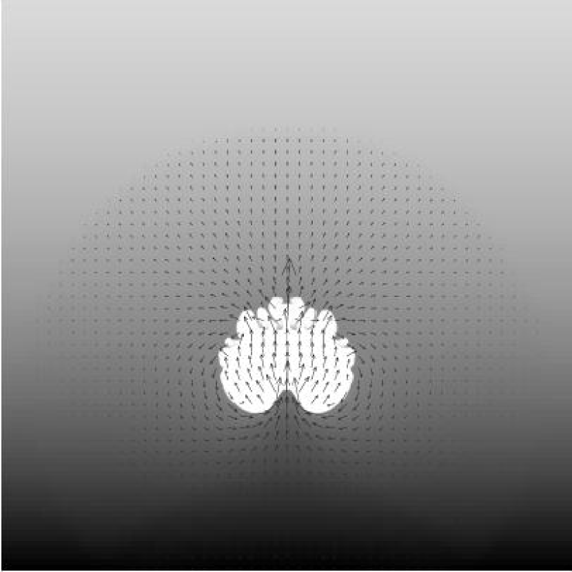
Figure 2: A plot of the velocity field around the bubble in the fiducial case (Fig. 1) at time $t\approx 72~{}\mathrm{Myr}$. Of particular note is the two emerging large-scale rolls on either side of the bubble, which will eventually form a stagnation line under the bubble, generating the high-density ‘tail’.

In the absence of magnetic effects, nothing prevents the complete disruption of the bubble. The bubble’s motion itself generates vortical motion in the surrounding fluid of the same size as the bubble and with rise velocity of the bubble, as shown in Fig. 2. These motions will then be able to rip the bubble apart on order of a bubble rise time, $t_{R}=\sqrt{4R/|g|}$, with $R$ being the bubble’s radius, and $g$ being the local gravitational acceleration. These effects have been studied previously (e.g., Harper 1972 and Layzer (1955)).

The bubble will also be susceptible to growth of the Rayleigh-Taylor instability at the top. Since we are dealing with large density contrasts, the Rayleigh-Taylor growth time (from linear theory) will be $t_{RT}=1/\sqrt{kg}=\sqrt{R/(2\pi gn)}$ for the mode that is $1/n$ the size of the bubble; however, modes of size on order the bubble radius, or small modes near the sides of the bubble will be suppressed because of the geometry of the bubble. Comparing time scales, the Rayleigh-Taylor instability will disrupt the bubble on small scales near the center of the bubble quickly, but the disruption of the entire bubble will be caused by induced vortical motions in the fluid. The shear along the side of the bubble will also be unstable to the Kelvin-Helmholtz instability; this will generate secondary instabilities as the evolution progresses.

The large scale motions of the fluid can be seen in Fig. 2 at time $t\sim 70~{}\mathrm{Myr}$. Two large rolls extend out, and their convergence under the bubble results in an up-welling and compression of material, forming a slight high-density tail in the wake of the bubble.

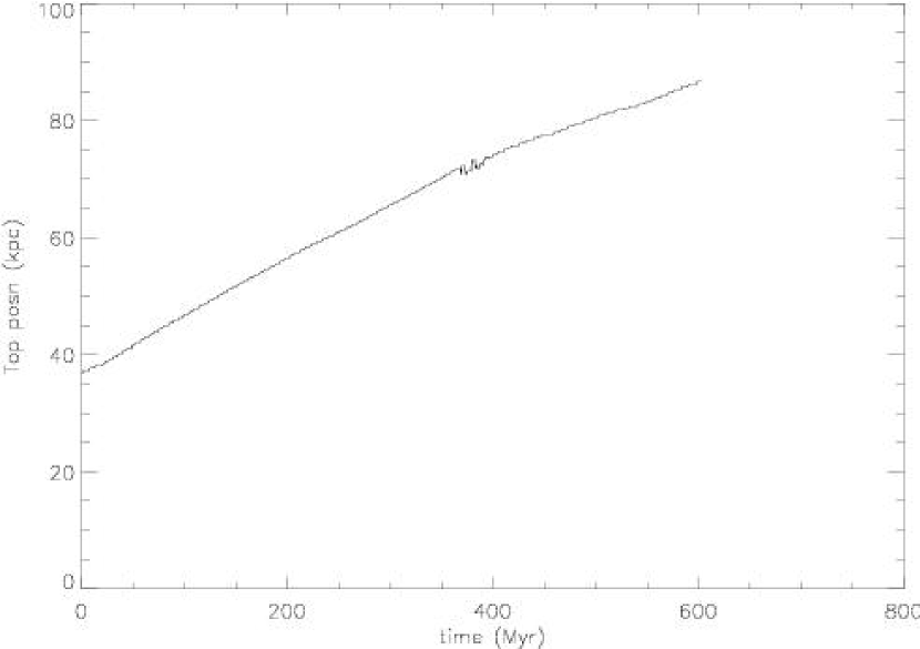
Figure 3: The position of the top of the rising bubble in our reference bubble case as shown in Fig. 1. After an initial acceleration, the bubble begins to slow down as it rises as both its relative buoyancy changes and it entrains heavier material from the environment. The irregularity at $t\approx 375\mathrm{Myr}$ is due to vortical motions pulling down the clump that had been the head of the bubble; some indication of this is shown in the middle frame of Fig. 1.

The position of the bubble top as a function of time is shown in Fig. 3. This position was calculated by horizontally averaging density throughout the domain and finding the first position from the top of the domain of a density jump; this local drop in density represents the presence of an under-dense fluid. Because our underdensities were so large, the position measured this way was insensitive to the precise value of the threshold we chose to mark the density jump. This measure allows us to track the top of a ‘bubble’ even when no coherent bubble exists. The bubble slows down over time primarily due to the entrainment of material from the environment as the bubble is disrupted.

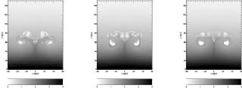
Figure 4: The state of the bubble at $t\approx 580~{}\mathrm{Myr}$ as resolution is decreased; at right, the reference case; middle, with resolution decreased to 3/8 of the full resolution ($192\times 240$); right, with resolution decreased to 3/16 ($96\times 120$). Plotted is density.

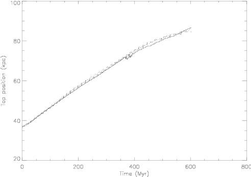
Figure 5: The position of the top of a $r=9\mathrm{kpc}$ bubble vs time for three resolutions. Solid line the resolution used in this study; dotted line decreased to a factor of 3/8; and dashed line decreased to a factor of 3/16.

As resolution varies, the small-scale structure varies, but the overall behavior remains the same, as is shown in Fig. 4 and Fig. 5. In these simulations, there is no modeled dissipation mechanism such as viscosity or thermal or material diffusion. In this case, only the numerical dissipation on small scales limits the amount of small scale structure. The small scale structure affects entrainment of ambient (denser) material, so that as resolution increases and numerical dissipation decreases, late-time heights change, but the early behavior is nearly identical.

A typical rise velocity for the still largely intact bubble can be seen from looking at the early-time slope in Fig. 3; it is approximately $0.1~{}\mathrm{kpc}~{}\mathrm{Myr}^{-1}$. That this is near the sonic velocity ($0.41~{}\mathrm{kpc}~{}\mathrm{Myr}^{-1}$) is not a coincidence. The density contrasts we consider here are large enough that the buoyant acceleration felt by the bubble is approximately $g$; since in an isothermal atmosphere the scale height is $H=c_{s}^{2}/(\gamma g)$, where $c_{s}$ is the sound speed, the velocity that the bubble picks up as it rises a significant fraction of a scale height is on the order $c_{s}$. The disruption of the bubble and entrainment of denser material before a scale height is reached prevents the bubble from accelerating past the sound speed.

3.1 Effects of Density Contrast

We ran simulations with density contrasts between the bubble and the maximum density in the box of 100:1 and 10:1. While there are some differences between the resulting structures (compare Figs.1 and 6), caused partly by the different growth of the Rayleigh-Taylor instability at the top of the bubble, the underlying dynamics are broadly similar. One way of understanding this is that in both cases, the bubble densities are very much less than the surrounding environment, so that it is the momentum of the fluid in the environment, not the bubble, which dominates the dynamics. Quantitatively, the Atwood number, $A=(\rho_{1}-\rho_{2})/(\rho_{1}+\rho_{2})$ is $0.82$ in the 10:1 case, and $0.98$ in the 100:1 case – so while the bubble density changes by a factor of 10, the Atwood number, which controls both the buoyant force and the evolution of the Rayleigh-Taylor instability, changes only by 20%.

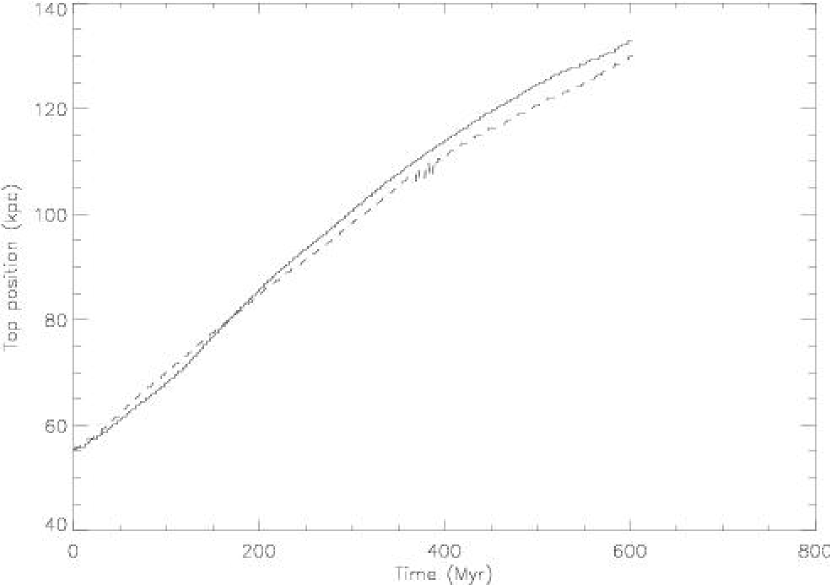
Figure 7: The position of the top of a rising bubble as shown in Fig. 3 (dashed line) and with the same parameters except a lower, 10:1, density contrast (solid line).

In particular, looking at the position of the top of the bubble versus time (in Figs. 3 and 7) we see a very similar evolution after the initial acceleration phase. Perhaps surprisingly, the bubble with the larger density (the 10:1 case) actually rose slightly further during the course of the simulation. In the late-time evolution, it is the entrainment of higher-density fluid which determines the buoyancy, and thus the acceleration, of the bubble. The bubble in the 10:1 case entrained less ambient fluid, thus its buoyancy ended up being greater than in the nominally more buoyant 100:1 case.

3.2 Effects of Geometry

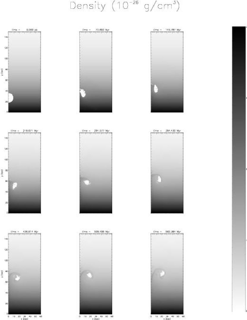
Figure 8: The evolution of a 9 $\mathrm{kpc}$ radius bubble in a 100:1 density contrast in cylindrical coordinates. The bubble is torn into two tori with a train of higher density material. Plotted is density.

In the purely hydrodynamic case it is possible to perform the same simulations described above in 2-D axisymmetric cylindrical coordinates, making the bubble a sphere instead of a cylinder. In this more physically relevant case, the bubble deforms into tori (Fig. 8), rather than the wing-like shape found in planar coordinates, as the shedded vorticity from the bubble rising becomes a vortex ring rather than two parallel lines of vorticity.

Because in this geometry there is less volume near the center of the bubble than there is towards the edges, the vortices that form can advect essentially all of the material from within the bubble into the vortex structure, so that the bubble becomes a rising vortex ring which then undergoes secondary instabilities. Also because of the geometry, the effect of the initial Rayleigh-Taylor instability in disrupting the bubble is diminished, although it does not vanish; the material that is disrupted by the Rayleigh-Taylor instability forms a smaller, secondary vortex ring that leads the larger ring.

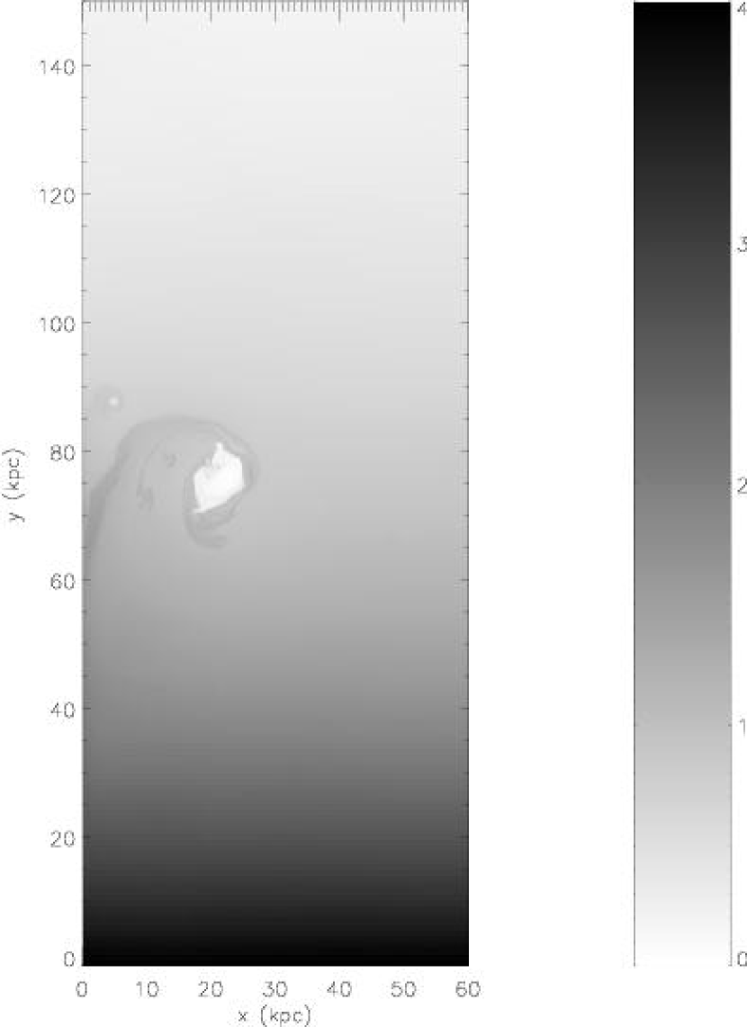
Figure 9: The effect of differing density contrasts for the simulations in cylindrical symmetry. Left, 10:1; right, 100:1. Frames are taken at time $t\approx 580~{}\mathrm{Myr}$. Density is plotted.

This simulation was performed with several density differences which all exhibited similar behavior. Fig. 8 shows the evolution of one of these cylindrical cases with a density contrast of 100:1 and a 9 $\mathrm{kpc}$ radius bubble. Fig. 9 shows the final frame of this simulation along with the corresponding frame of a simulation performed with a 10:1 density contrast. As with the planar case, although there are differences in the small-scale structure, the medium- and large-scale behavior is essentially unchanged.

3.3 Effects of Bubble Size

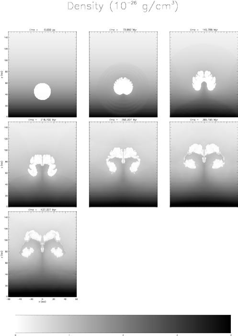
Figure 10: The evolution of a $r=15~{}\mathrm{kpc}$ bubble in a 100:1 density contrast, $g=-7\times 10^{-9}\mathrm{cm\ s^{-2}}$ atmosphere. The Raleigh-Taylor instability grows much further in this case, as there are more modes to grow on the larger bubble. The larger growth rate means that significant evolution has occurred before the induced vortical motions begin to rip the bubble apart in earnest; thus there is a much larger ‘head’ to the structure than in the base case in Fig. 1. The simulation was ended early as the bubble approached the boundaries of the domain. Density is plotted.

Simulations were also performed with a larger and a smaller bubble in the planar case. In the case of the larger $r=15\ \mathrm{kpc}$ bubble of Fig. 10, the Raleigh-Taylor instability plays a much larger role in the evolution of the bubble than in the previous case, as there are more modes that can grow on the larger top of the bubble. Conversely, the $r=10\ \mathrm{kpc}$ bubble (Fig. 11) tends to remain flat across the top, and is primarily disrupted by the induced vortical motions.

3.4 Effects of Stratification

The isothermal atmosphere surrounding the bubble has an exponential density profile provided by a constant gravitational field in the negative $y$-direction. Changing the stratification, through the gravitational acceleration, has two major effects. Immediately, it changes the time scale on which the dynamics occurs, as shown in the scaling relations in §2. The stratification also tends to elongate vortical motions in the atmosphere, due to lower densities at higher positions.

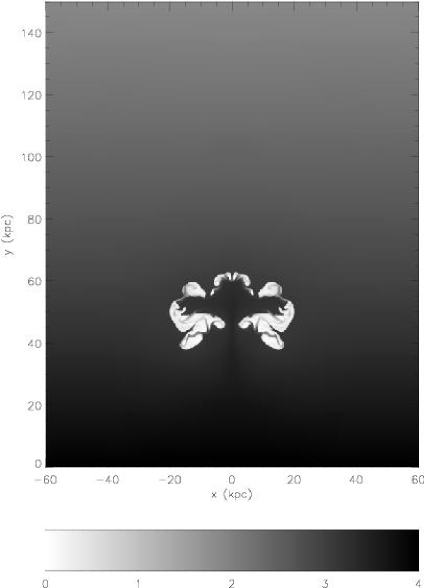
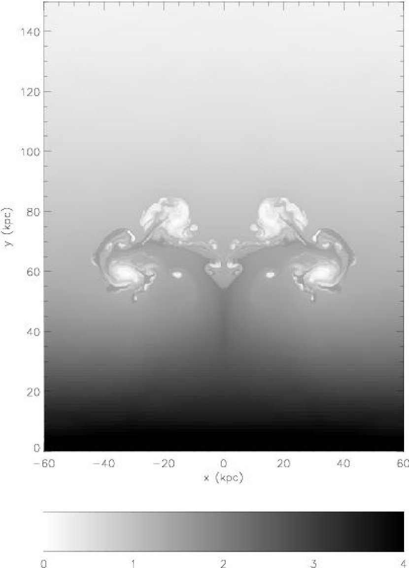
Figure 13: The effect of stratification on the evolution of the bubble; shown at left is the density field for the simulation with $g=-1.75\times 10^{-9}\mathrm{cm\ s^{-2}}$ at $t\approx 580\ {\mathrm{Myr}}$, and on the right, that for $g=-7\times 10^{-9}\mathrm{cm\ s^{-2}}$ at $t\approx 290\ {\mathrm{Myr}}$. Plotted is density.

In Fig. 12 we show the evolution of a bubble moving through a less stratified domain, with the gravity set to be one quarter of its value in our reference case. In Fig. 13, we compare the final frame of the evolution with the frame from the corresponding time (taking into account the change of the buoyant time scale) of our reference case.

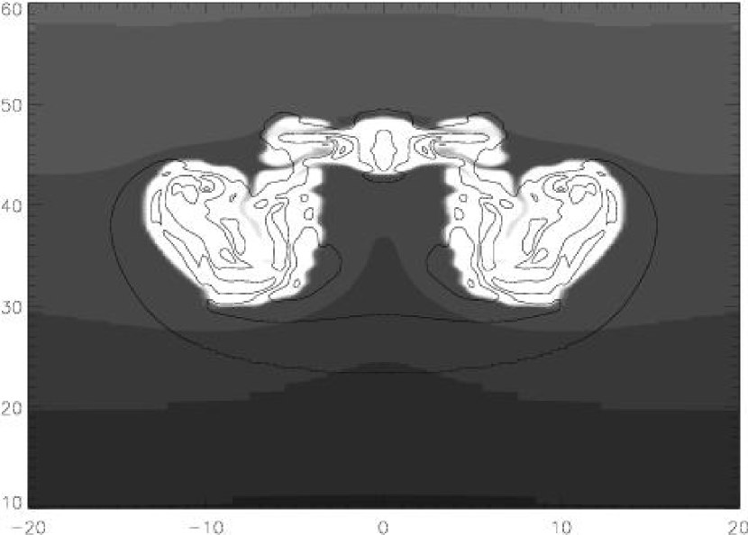
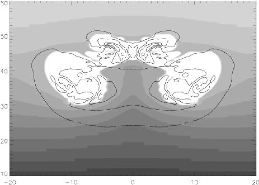
Figure 14: Scaled total velocity contours superimposed on the density field; shown at left are results for the simulation with $g=-1.75\times 10^{-9}\mathrm{cm\ s^{-2}}$ at $t\approx 290\ {\mathrm{Myr}}$, and on the right, that for $g=-7\times 10^{-9}\mathrm{cm\ s^{-2}}$ at $t\approx 145\ {\mathrm{Myr}}$. In the more strongly stratified case (on the right), the velocity contours extend further up than in the less stratified case.

Some of the differences between the two simulations can be understood in terms of the height of the vortical motions induced by the rising bubble. The large-scale motions, if they are to conserve momentum, must be elongated in atmospheres where the density is stratified, as there is less mass at higher positions in the atmosphere. Fig. 14 shows total velocity contours on top of a zoom-in of density for the same simulations as in Fig. 13, but at earlier times. The vortical motions extend noticeably higher in the more stratified case, meaning that in this case the bubble will be disrupted over longer length scales.

4 MAGNETIC FIELDS: HOT BUBBLE IN A BACKGROUND FIELD

From purely hydrodynamic bubbles, we move on to examining hot bubbles rising in a fluid with an initially constant background field running through the entire domain. In the rest of this paper, we describe solutions performed with the MHD solver in the Flash code. The rest of the code, including the boundary conditions and initialization, remained unchanged; the MHD solver was simply compiled into the simulation code in place of the PPM solver. This MHD solver is based on the code described in Powell et al. (1999), with two methods of ‘$\nabla\cdot{\bf{B}}$-cleaning’ – a diffusive method due to Marder (1987), and a projection method due to Brackbill and Barnes (1980). We used the diffusive mechanism for the results described here due to the more modest computational cost of this method and the simple magnetic dynamics in these simulations. Our implementation of this MHD solver works only in Cartesian coordinates, so we consider only the 2-D planar cases.

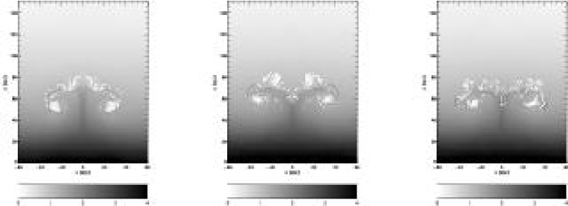
Figure 15: Left, the small scale structure at 580 $\mathrm{Myr}$ using the MHD solver with no magnetic field. Center, the small scale structure at the same time calculated with the PPM solver. Right, the small scale structure at the same time using the PPM solver with linear, rather than parabolic, reconstruction functions more similar to that used by the MHD solver. Plotted is density.

Since we are changing the numerical solver as well as adding magnetic fields to the initial conditions, it is important to ensure that we get the same results in the purely hydrodynamic case with both solvers. Calculating our reference case without magnetic fields with both solvers, we find noticeable, but understandable, differences in the final results. Shown in Fig. 15 is our reference calculation at the final time calculated with our MHD solver and the same result with the PPM solver. The MHD result looks something like the lower-resolution versions of the PPM solution (Fig. 4), which can be understood to be a consequence of the the lower spatial order of accuracy of the MHD solver. Fig. 15 also shows the results of using the purely hydrodynamic solver with reconstruction functions more similar to those in the MHD solver, which improves the agreement between the simulations. Understanding the differences between the results of the different solvers gives us some confidence that the results obtained with the magnetic field solver can be meaningfully compared with those calculated using the purely hydrodynamic solver.

In the results that follow, a density ratio of 10:1 was used. This avoids numerical issues which can arise if there is too large a jump in Alfvén velocity across a small region (eg., between the bubble and the ambient material.)

4.1 Horizontal Field

4.1.1 z-field

The simplest case to consider in 2-D is an initial magnetic field in the $\bf{\hat{z}}$-direction, out of the plane of the simulation domain. In this case, the magnetic field lines can slip around the cylinder as it rises, enhancing the initial production of large-scale vorticity around the bubble. The magnetic field’s contribution to the dynamics in this case is simply as an additional, constant, pressure term $B^{2}/(8\pi)$, reducing the effective relative pressure stratification $\nabla p/p$ by a factor of $\beta_{0}/(\beta_{0}+1)$ while leaving the density structure unchanged. Here $\beta_{0}$ is the plasma $\beta$ parameter (gas pressure divided by magnetic pressure) at the base of the atmosphere. This effective pressure scale height will be one characteristic length scale for eddies, so that decreasing $\beta$ will, up to a limit, decrease the characteristic vortical motion size without the elongation that increasing the density stratification would produce.

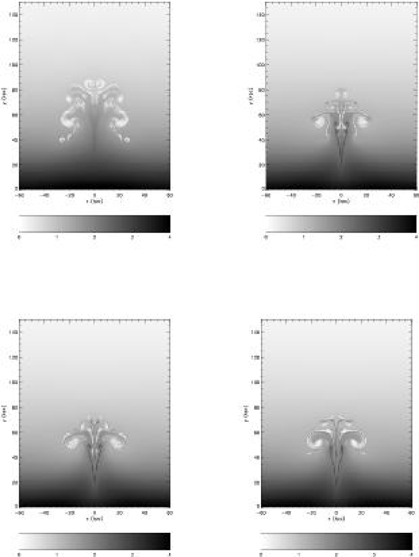
Figure 17: The state at time $t\approx 580~{}\mathrm{Myr}$ of a bubble rising in a medium with a constant magnetic field in the $\bf{\hat{z}}$ direction with $\beta_{0}=462$ (top left), $0.185$ (top right), $0.046$ (bottom left), and $0.012$ (bottom right). The panels are plots of density.

The evolution of a bubble in a very weak $\bf{\hat{z}}$-field is shown in Fig. 16. In Fig. 17 is shown the final frame for simulations with $\beta_{0}$ of 462, 0.19, 0.046, and 0.012. As $\beta_{0}$ decreases, the vortical structures are seen to ‘tighten’.

At late times, the high-density wake that the bubble leaves begins to contain low-density structures; one explanation for this is that the large-scale motions induced by the flow sweep up magnetic field lines, resulting in a higher magnetic field density in the wake of the bubble; the resulting increase in magnetic pressure means a lower mass density under these constant-pressure conditions, leaving a different tail in this case than in the purely hydrodynamic case.

4.1.2 x-field

As opposed to the effects of a field in the $\bf{\hat{z}}$-direction, even an extremely weak field in the $\bf{\hat{x}}$ direction in this geometry can strongly contain the rising bubble in our planar coordinates. We see from Chandrasekhar (1981) that the magnetic field suppresses the Kelvin-Helmholtz instability completely unless the relative velocity between the bubble and the ambient medium exceeds the root-mean square Alfvén speed in the two media; or, as written in Vikhlinin et al. (2001),

$$4\pi\frac{\rho_{0}\rho_{b}}{\rho_{0}+\rho_{b}}v^{2}>B^{2}_{0}+B^{2}_{b}.$$ (13)

At the top of the bubble, near the stagnation point, the relative velocity is nearly zero and of course the instability is suppressed. Even near the sides, however, because the Alfvén speed in the bubble is so high (due to the low density), the shear velocity would have to be many times the ambient Alfvén speed to for Kelvin-Helmholtz instabilities to occur.

Initially, since $B_{0}=B_{b}$, this reduces to $\beta_{0}>(4/\gamma)(\rho_{0}/\rho_{b}+1){\cal M}^{-2}$ where $\gamma$ is the ratio of specific heats for the gas, and ${\cal M}$ is the flow Mach number. Since we have a density ratio of 10:1, a Mach number of 0.25, and a 5/3-law ideal gas, this suggests that for $\beta_{0}>420$, the bubble should be unstable to shear. However, we show the evolution of a bubble with $\beta_{0}=462$ in Fig. 18, and there is clearly no shear instability present. In fact, as the bubble rises, not only does shear occur but the magnetic field lines are wrapped around the rising bubble, increasing the field density. Further, the shear at the bubble interface is overestimated by the net bubble velocity upwards. Applying Eq. 13 to the data of Fig. 18, we find that the shear everywhere is several orders of magnitude below the threshold for instability. This is tabulated in Table 1.

In this case of a horizontal magnetic field, the wake left behind by the bubble is an unstructured high-density entrained tail; this will be true in the spherical bubble case, as it is caused by the stagnation line caused by the induced vortical motions of the rising bubble.

The drastically different effects of the two horizontal orientations of the uniform magnetic field is partly an artifact of the geometry of the simulation. For a spherical bubble, rather than a cylindrical bubble, a uniform horizontal field would act on the bubble asymmetrically – as a tension in one plane, and as a pressure component in the other. In particular, the strong containing effect of even a weak $\bf{\hat{x}}$-field is a geometrical artifact of these simulations.

4.2 Vertical Field

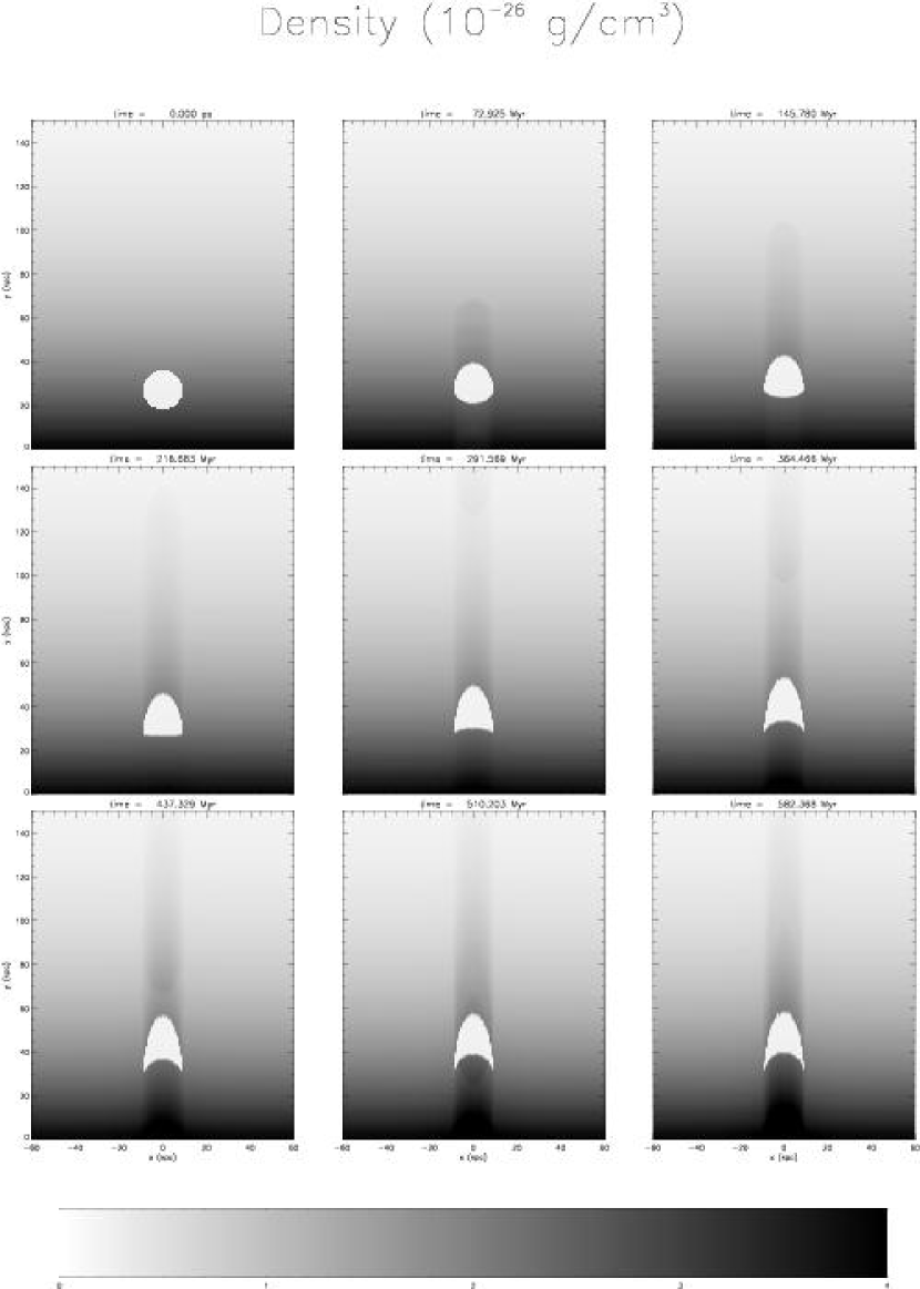
Figure 20: The evolution of a bubble in a vertically magnetized background plasma, $\beta_{0}=.019$. The panels are plots of density.

A vertical field has a more direct dynamical effect on the rising bubble. Adding a weak vertical field does not prevent the bubble from breaking up, but somewhat suppresses the cascade of vortical motions at late times by suppressing horizontal motions as compared to vertical motions (Fig. 19). If we increase the strength of the magnetic field, however, the suppression of horizontal motions can be so strong that the bubble is deformed into a chevron and travels upwards intact (Fig. 20.) A sufficiently strong vertical magnetic field can completely contain the bubble, although it is difficult to imagine a cluster having a magnetic field of this magnitude over the entire size of the observed bubbles.

5 MAGNETIC FIELDS: MAGNETIZED BUBBLE IN A BACKGROUND FIELD

In the previous sections, under-dense bubbles were supported by thermal pressure. This isotropic thermal pressure can support the bubble against collapse, but not against being torn apart by the fluid motions induced by its own rising. The ambient magnetic fields could only prevent this if the fields were strong enough (or oriented fortuitously) to suppress those large-scale fluid motions. We now consider bubbles which are supported instead by magnetic fields, which provide an anisotropic ‘pressure’ support that also acts as a tension; this tension can be enough to maintain the bubble even in the presence of such motions.

One can construct families of solutions to the MHD equations with the property that $\vec{B}$ is force-free (i.e. $\vec{J}\times\vec{B}=0$) everywhere in the domain except at the boundary between the under-dense bubble and the ambient medium, where the Lorentz force balances the gas pressure jump. We choose a field used in Cargill and Chen (1996) for flux tubes:

$$B_{\theta} = \cases{B_{b}\frac{r}{a_{0}}&$r\leq a_{0}$,\cr 0&$r>a_{0}$.\cr}$$ (14)

$$B_{z} = \cases{B_{b}\sqrt{4-2\left(\frac{r}{a_{0}}\right)^{2}}&$r\leq a_{0}$,\cr B_{z0}&$r>a_{0}$.\cr}$$ (15)

$$B_{b} = \sqrt{\frac{8\pi}{3}p_{0}\left(1-\frac{\rho_{b}}{\rho_{0}}\right)+B_{z0}^{2}}.$$ (16)

Here $p_{0}$ is the ambient gas pressure, $\rho_{0}$ is the ambient gas density, $\rho_{b}$ is the gas density inside the bubble, $B_{z0}$ is the ambient magnetic field in the $\bf{\hat{z}}$ direction, and $a_{0}$ is the radius of the bubble. Thus we have a uniform magnetic field in the ${\bf{\hat{z}}}$ direction in the ambient medium, as discussed in our previous section, but the bubble is also supported by an azimuthal field and an enhanced ${\bf{\hat{z}}}-$field.

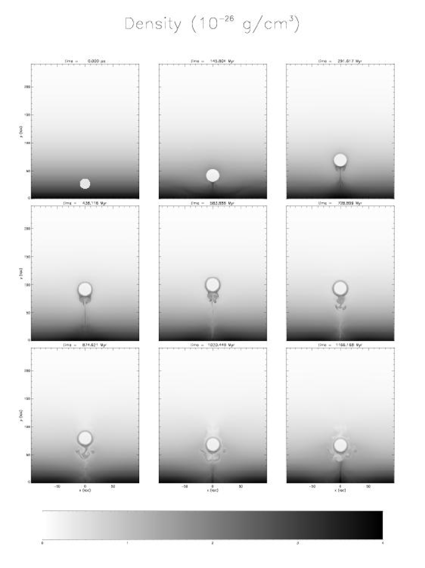
Figure 21: The evolution of the magnetically supported bubble as it rises without being torn apart. The panels are plots of density. This simulation was run for a longer time; a larger domain was used so that the bubble could rise without being interfered with by the top boundary.

The hydrodynamic initial conditions are computed as in previous sections, except that in this case the underdense region is at the same temperature as the background material, and a constant Lorentz force at the bubble interface supports the bubble against the larger external ambient pressure. The evolution is shown in Fig. 21. In this case, the bubble maintains its form as it rises.

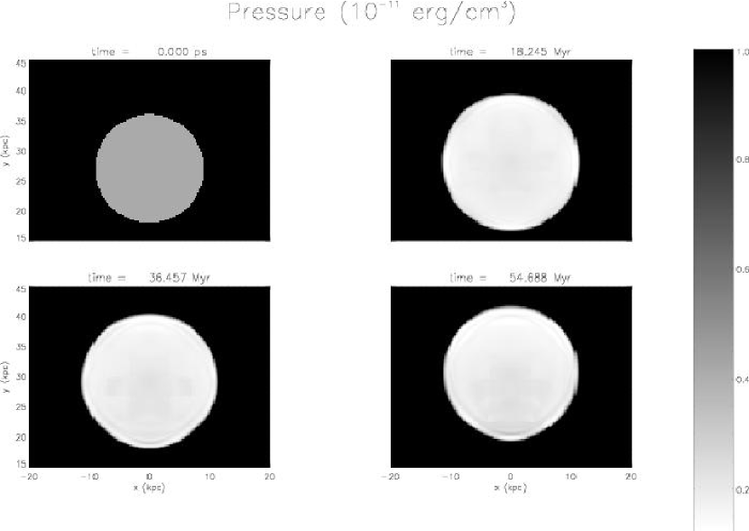
Figure 22: The short-time evolution of the gas density inside the magnetic bubble as it settles into an equilibrium. The bubble expands and the gas inside the bubble is distributed towards the bottom of the bubble.

Because the ambient pressure changes by approximately 30% over the height of the bubble, while the bulk of the pressure support of the bubble is fixed by the magnetic field jump, a transient occurs over the course of a few sound-crossing times of the bubble (that is, a few times 44 $\mathrm{Myr}$) as the bubble equilibrates; the short-time evolution of gas pressure is is shown in Fig. 22. The magnetic field is enough to maintain the bubble’s shape until gas pressure and density inside the bubble is redistributed to maintain equilibrium; we see in Fig. 22 that the bubble expands overall, and gas slightly settles towards the bottom.

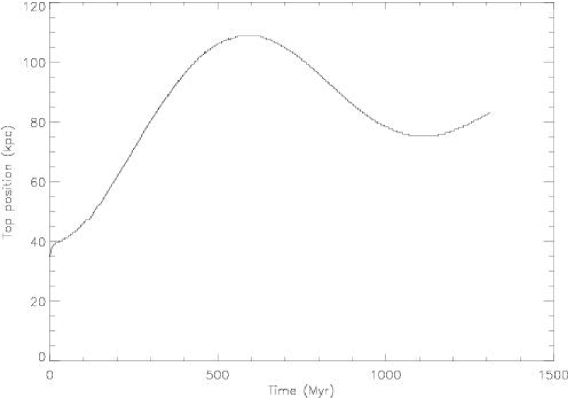
Figure 23: The magnetically supported bubble rises until it passes it’s point of neutral buoyancy then falls again, and again overshoots.

The bubble adiabatically expands as it rises, and eventually overshoots the height of neutral buoyancy, decelerates, and falls back again (Fig. 23). We also see again at late times the development of an under-dense wake as in the uniform ${\bf{\hat{z}}}$-field case.

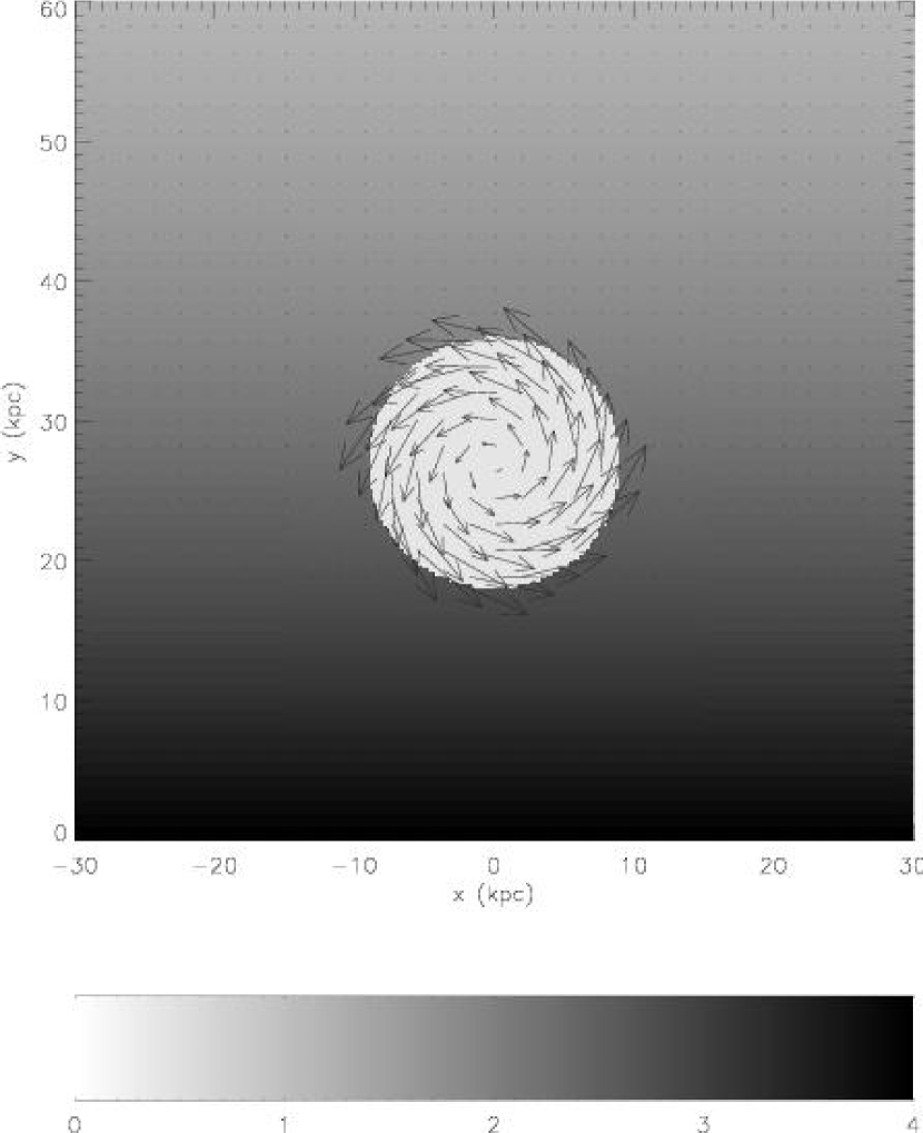
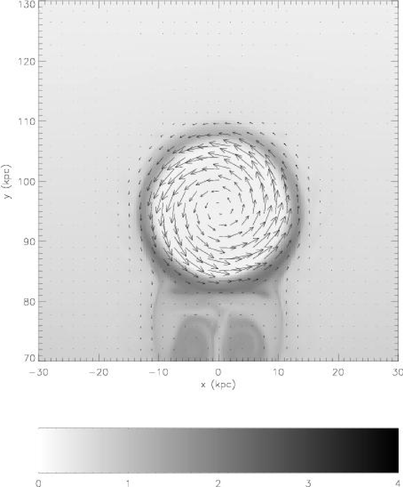
Figure 24: Azimuthal field vectors, plotted over the density field, inside bubble and collar at t=0 and t=580 Myr.

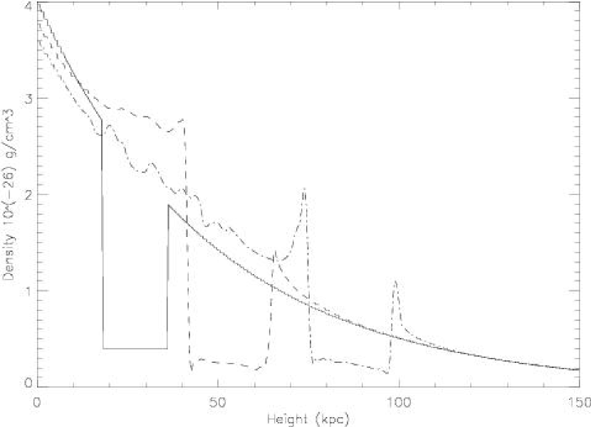
Figure 25: Vertical density profiles (through $x=0$) of the magnetized bubble simulation, taken at times $t=0,220,440\mathrm{Myr}$ (solid line, dashed line, dot-dashed line).

Also notable is that the bubble carries a ring of higher density material (Fig. 24). Such a high-density ring has also been noted in Chandra observations of bubbles. This collar of material appears to be “grabbed” by the azimuthal field at time t=0 when the entire bubble is surrounded by higher density material. As shown in Fig. 25, the high density collar surrounding the low-density bubble does not change in density significantly as the bubble moves upwards, suggesting that the bubble simply advects ambient material.

6 CONCLUSIONS

This work focused on examining the primary physical conditions that have to occur for the continued existence of the dark spots in galaxy clusters found by the Chandra X-ray observatory. We confirm that bubbles without supporting magnetic fields are torn apart by instabilities and vortical motions before they can move an entire bubble height. This is surprising, as ‘ghost’ bubbles — not radio bright, and thus presumably no longer powered — are observed (Mazzotta et al., 2002; Fabian et al., 2000; McNamara et al., 2000) which are a significant distance in bubble lengths away from the radio source which presumably formed them. The existence of these bubbles can be explained if they are supported by an internal magnetic field.

Furthering this argument is the importance of thermal diffusion absent any magnetic field effects. One can numerically integrate the diffusion equation using the thermal diffusivity quoted in §2 given by Spitzer (1962). On doing so, one finds that an $r=9~{}\mathrm{kpc}$ bubble at a temperature of 100 $\mathrm{keV}$ in an ambient gas of 1 $\mathrm{keV}$ is largely diffused away after 1 $\mathrm{Myr}$; a 10 $\mathrm{keV}$ bubble survives for perhaps 150 $\mathrm{Myr}$. Indeed, if the Spitzer diffusivity is appropriate, there are constraints much tighter than this; the Chandra observations show a sharp edge to the bubble, and this edge would be blurred by thermal diffusion on time scales orders of magnitude shorter than those required to completely dissipate the bubble.

Thermal arguments alone, however, are not enough to require a magnetic field to support the bubble; a weak tangled magnetic field may reduce the conductivity without being strong enough to support the bubble, for instance, or one could require more sophisticated diffusivities in the presence of such large gradients than the Spitzer model. In addition, the synchrotron emission in the bubble may suggest that a 10-100 $\mathrm{keV}$ thermal gas is an insufficient model for the gas inside the bubble.

This research also suggests that the ring of brighter material surrounding these bubbles may be caused by magnetic diffusion of the field that maintains them. There is also numerical evidence suggesting a wake left behind the bubble as it moves. Searching the radio emissions for such a wake would be a good indicator as to whether or not these bubbles are moving.

Since magnetic fields may be necessary to keep the bubbles intact as they travel, future work should focus on MHD simulations, and in particular performing simulations with more physically meaningful geometry than 2D planar symmetry. As was seen in the hydrodynamic case, the difference between cylindrical and planar geometry significantly altered the morphology, if not the timescale, of the disruption of the bubble; the difference in geometries would be even more pronounced in the presence of magnetic fields, since the orientation of the field also plays a role. The hot bubble in magnetic field simulations generalize easily to 3D; the magnetized bubble simulation will be more complicated, as one can not write down an analytical magnetic field in 3D which would support a spherical bubble analogous to the cylindrical flux-tube presented here. Such a field, numerically generated, however, should also be able to support the bubble without disruption. Including the divergent geometry appropriate to the center of a cluster will also be a necessary step.

Figure 1: The time evolution of our ‘standard’ bubble case - $g=-7\times 10^{-9}\mathrm{cm\ s^{-2}}$, density contrast of 100:1, peak density of $\rho=4\times 10^{-26}\mathrm{g\ cm^{-3}}$, 3.1 pressure scale heights in the 2-D planar domain, and bubble radius of $9~{}\mathrm{kpc}$. Plotted is density.

Figure 6: The time evolution of the 10:1 density contrast case. Shown in the panels is density.

Figure 11: The evolution of a $r=6~{}\mathrm{kpc}$ bubble in the 100:1 density contrast, $g=-7\times 10^{-9}\mathrm{cm\ s^{-2}}$ case. Plotted is density.

Figure 12: The evolution of a $r=9~{}\mathrm{kpc}$ bubble in a less-stratified atmosphere, with $g=-1.75\times 10^{-9}~{}\mathrm{cm\ s^{-2}}$. Plotted is density.

Figure 16: The time evolution of a 10:1 bubble rising in a constant initial background magnetic field in the $\bf{\hat{z}}$-direction (out of the plane of the paper) with $\beta_{0}=462$. Plotted is density.

Figure 18: The evolution of a bubble in a horizontally magnetized background plasma with magnetic field in the ${\bf{\hat{x}}}$-direction, $\beta_{0}=462$. Plotted is density.

Time (Myr)	$v_{s}$	$\frac{B_{s}}{B_{0}}$	$\frac{B_{s}}{B_{\mathrm{stable}}}$
73	0.014	1.1	$3.51\times 10^{4}$
150	0.027	2.8	$9.58\times 10^{4}$
220	0.130	3.8	$2.86\times 10^{4}$
290	0.109	6.4	$3.56\times 10^{4}$
370	0.090	6.1	$3.46\times 10^{4}$
440	0.094	5.7	$3.12\times 10^{4}$
510	0.081	3.0	$1.71\times 10^{4}$
580	0.066	2.0	$3.14\times 10^{4}$

Table 1: Shearing and stability data for horizontal $\beta_{0}=462$ simulation. Tabulated is the time for which the data was taken, a mean shear velocity (in $\mathrm{kpc}$/$\mathrm{Myr}$), a mean enhancement of the magnetic field at the shear layer, and the factor by which the magnetic field is greater than the stabilizing magnetic field.

Figure 19: The evolution of a bubble in a vertically magnetized background plasma, $\beta_{0}=462$. The panels are plots of density.

References

- Allen et al. [2001] S. W. Allen, G. B. Taylor, P. E. J. Nulsen, R. M. Johnstone, L. P. David, S. Ettori, A. C. Fabian, W. Forman, C. Jones, and B. McNamara. Chandra X-ray observations of the 3C 295 cluster core. MNRAS, 324:842–858, July 2001.
- Basson and Alexander [2003] J. F. Basson and P. Alexander. MNRAS, 339:353–359, 2003.
- Blanton et al. [2003] E. L. Blanton, C. L. Sarazin, and B. R. McNamara. ApJ, 585:227–243, 2003.
- Böhringer et al. [2002] H. Böhringer, K. Matsushita, E. Churazov, Y. Ikebe, and Y. Chen. A&A, 382:804–820, 2002.
- Brackbill and Barnes [1980] J. U. Brackbill and D. C. Barnes. The Effect of Nonzero on the Numerical Solution of the Magnetohydrodynamic Equations. J. Comp. Phys., 35:426–430, 1980.
- Brandenburg and Hazlehurst [2001] A. Brandenburg and J. Hazlehurst. A&A, 370:1092–1102, 2001.
- Brüggen [2003] M. Brüggen. Simulations of Buoyant Bubbles in Galaxy Clusters. ArXiv Astrophysics e-prints, 0301352, January 2003.
- Brüggen and Kaiser [2001] M. Brüggen and C. R. Kaiser. Buoyant radio plasma in clusters of galaxies. MNRAS, 325:676–684, 2001.
- Brüggen et al. [2002] M. Brüggen, C. R. Kaiser, E. Churazov, and T. A. Enßlin. MNRAS, 331:545–555, 2002.
- Brüggen and Kaiser [2002] Marcus Brüggen and Christian R. Kaiser. Hot bubbles from active galactic nuclea as a heat source in cooling-flow clusters. Nature, pages 301–303, July 2002.
- Calder et al. [2002] A. C. Calder, B. Fryxell, T. Plewa, R. Rosner, L. J. Dursi, V. G. Weirs, Dupont T., H. F. Robey, J. O. Kane, B. A. Remington, R. P. Drake, G. Dimonte, M. Zingale, F. X. Timmes, K. Olson, P. Ricker, P. MacNeice, and H. M. Tufo. On validating an astrophysical simulation code. ApJS, 143:201–230, December 2002.
- Cargill and Chen [1996] P. J. Cargill and J. Chen. Magnetohydrodynamic simulations of the montion of magnetic flux tubes through a magnetized plasma. Journal of Geophysical Research, 101:4855–4870, March 1996.
- Cavaliere and Fusco-Femiano [1976] A. Cavaliere and R. Fusco-Femiano. X-rays from hot plasma in clusters of galaxies. A&A, 49:137–144, May 1976.
- Chandrasekhar [1981] S. Chandrasekhar. Hydrodynamic and Hydromagnetic Stability. Dover, New York, 1981.
- Churazov et al. [2001] E. Churazov, M. Brüggen, C. R. Kaiser, H. Böhringer, and W. Forman. ApJ, 554:261–273, 2001.
- Ensslin and Heinz [2002] T.A. Ensslin and S. Heinz. Radio and x-ray detectability of buoyant radio plasma bubbles in clusters of galaxies. A&A, 384:L27–30, March 2002.
- Fabian [1994] A. C. Fabian. Cooling Flows in Clusters of Galaxies. ARA&A, 32:277–318, 1994.
- Fabian et al. [2000] A. C. Fabian, J. S. Sanders, S. Ettori, G. B. Taylor, S. W. Allen, C. S. Crawford, K. Iwasawa, R. M. Johnstone, and P. M. Ogle. Chandra imaging of the complex X-ray core of the Perseus cluster. MNRAS, 318:L65–L68, November 2000.
- Forman et al. [2002] W. Forman, C. Jones, M. Markevitch, A. Vikhlinin, and E. Churazov. Chandra Observations of the Components of Clusters, Groups, and Galaxies and Their Interactions. In Lighthouses of the Universe: The Most Luminous Celestial Objects and Their Use for Cosmology Proceedings of the MPA/ESO, page 51, 2002.
- Fryxell et al. [2000] B. Fryxell, K. Olson, P. Ricker, F. X. Timmes, M. Zingale, D. Q. Lamb, P. MacNeice, R. Rosner, J. W. Truran, and H. Tufo. FLASH: An Adaptive Mesh Hydrodynamics Code for Modeling Astrophysical Thermonuclear Flashes. ApJS, 131:273–334, November 2000.
- Garnier et al. [1999] E. Garnier, M. Mossi, P. Sagaut, P. Comte, and M. Deville. On the Use of Shock-Capturing Schemes for Large-Eddy Simulation. J. Comp. Phys., 153:273–311, August 1999.
- Harper [1972] J. F. Harper. The motion of bubbles and drops through liquids. Adv. Appl. Mech, 12:59–129, 1972.
- Kaastra et al. [2001] J. S. Kaastra, C. Ferrigno, T. Tamura, F. B. S. Paerels, J. R. Peterson, and J. P. D. Mittaz. A&A, 365:L99–L103, 2001.
- Layzer [1955] David Layzer. On the instability of superposed fluids in a gravitiational field. ApJ, 122:1–23, July 1955.
- MacNeice et al. [2000] P. MacNeice, Kevin M Olson, Clark Mobarry, Rosalinda deFainchtein, and Charles Packer. Paramesh: A parallel adaptive mesh refinement community toolkit. Computer Physics Communications, 126:330–354, 2000.
- Magnaudet and Eames [2000] J. Magnaudet and I Eames. The motion of high-reynolds-number bubbles in inhomogeneous flows. Ann. Rev. Fluid Mech., 32:659–708, 2000.
- Marder [1987] Barry Marder. A method for incorporating gauss’ law into electromagnetic pic codes. J. Comp. Phys., 68:48–55, 1987.
- Matsushita et al. [2002] K. Matsushita, E. Belsole, A. Finoguenov, and H. Böhringer. A&A, 386:77–96, 2002.
- Mazzotta et al. [2002] P. Mazzotta, J. S. Kaastra, F. B. Paerels, C. Ferrigno, S. Colafrancesco, R. Mewe, and W. R. Forman. Evidence for a Heated Gas Bubble inside the “Cooling Flow” Region of MKW 3s. ApJ, 567:L37–L40, March 2002.
- McNamara et al. [2000] B. R. McNamara, M. Wise, P. E. J. Nulsen, L. P. David, C. L. Sarazin, M. Bautz, M. Markevitch, A. Vikhlinin, W. R Forman, C Jones, and D. E. Harris. Chandra x-ray observations of the hydra a cluster; an interaction between the radio source and the x-ray emitting gas. ApJ, 534:L135–L138, May 2000.
- McNamara et al. [2001] B. R. McNamara, M. W. Wise, P. E. J. Nulsen, L. P. David, C. L. Carilli, C. L. Sarazin, C. P. O’Dea, J. Houck, M. Donahue, S. Baum, M. Voit, R. W. O’Connell, and A. Koekemoer. Discovery of ghost cavities in the x-ray atmosphere of abell 2597. ApJ, 562:L149–L152, December 2001.
- Nulsen et al. [2002] P. E. J. Nulsen, L. P. David, B. R. McNamara, C. Jones, W. R. Forman, and M. Wise. Interaction of Radio Lobes with the Hot Intracluster Medium: Driving Convective Outflow in Hydra A. ApJ, 568:163–173, March 2002.
- Peterson et al. [2001] J. R. Peterson, F. B. S. Paerels, J. S. Kaastra, M. Arnaud, T. H. Reiprich, A. C. Fabian, R. F. Mushotzky, J. G. Jernigan, and I. Sakelliou. X-ray imaging-spectroscopy of Abell 1835. A&A, 365:L104–L109, January 2001.
- Porter and Woodward [1994] D. H. Porter and P. R. Woodward. High-resolution simulations of compressible convection using the piecewise-parabolic method. ApJS, 93:309–349, July 1994.
- Powell et al. [1999] Kenneth G. Powell, Philip L. Roe, Timur J. Linde, Tamas I. Gombosi, and Darren L. De Zeeuw. A Solution-Adaptive Upwind Scheme for Ideal Magnetohydrodynamics. J. Comp. Phys., 154:284–309, 1999.
- Reynolds et al. [2002] C. S. Reynolds, S. Heinz, and M. C. Begelman. The hydrodynamics of dead radio galaxies. MNRAS, 332:271–282, May 2002.
- Schmidt et al. [2001] R. Schmidt, S. W. Allen, and A. C. Fabian. MNRAS, 327:1057, 2001.
- Soker et al. [2002] N. Soker, E. L. Blanton, and C. L. Sarazin. Hot Bubbles in Cooling Flow Clusters. ApJ, 573:533–541, July 2002.
- Spitzer [1962] Lyman Spitzer. Physics of Fully Ionized Gasses. Interscience Publishers, New York, 2nd edition, 1962.
- Sun et al. [2003] M. Sun, C. Jones, S. S. Murray, S. W. Allen, A. C. Fabian, and A. C. Edge. Chandra Observations of the Galaxy Cluster A478: The Interaction of Hot Gas and Radio Plasma in the Core, and an Improved Determination of the Compton y-Parameter. ApJ, 587:619–624, April 2003.
- Sytine et al. [2000] I. V. Sytine, D. H. Porter, P. R. Woodward, S. W. Hodson, and K. Winkler. Convergence Tests for the Piecewise Parabolic Method and Navier-Stokes Solutions for Homogeneous Compressible Turbulence. J. Comp. Phys., 158:225–238, March 2000.
- Tamura et al. [2001] T. Tamura, J. S. Kaastra, J. R. Peterson, F. B. S. Paerels, J. P. D. Mittaz, S. P. Trudolyubov, G. Stewart, A. C. Fabian, R. F. Mushotzky, D. H. Lumb, and Y. Ikebe. X-ray spectroscopy of the cluster of galaxies Abell 1795 with XMM-Newton. A&A, 365:L87–L92, January 2001.
- Tucker and Rosner [1983] Wallace H. Tucker and Robert Rosner. Thermal conduction and heating by nonthermal electrons in the x-ray halo of m87. ApJ, 267:547–550, 1983.
- Vikhlinin et al. [2001] A. Vikhlinin, M. Markevitch, and S. S. Murray. Chandra estimate of the magnetic field strength near the cold front in a3667. ApJ, 549:L47–L50, March 2001.
- Zingale et al. [2002] M. Zingale, L. J. Dursi, J. Zuhone, A. C. Calder, B. Fryxell, T. Plewa, J. W. Truran, A. Caceres, K. Olson, P. M. Ricker, K. Riley, R. Rosner, A. Siegel, F. X. Timmes, and N. Vladimirova. Mapping initial hydrostatic models in godunov codes. ApJS, 143:539–565, Dec 2002.