Multipole Vectors—a new representation of the CMB sky
and evidence for statistical anisotropy or non-Gaussianity at $2\leq\ell\leq 8$

Abstract

We propose a novel representation of cosmic microwave anisotropy maps, where each multipole order $\ell$ is represented by $\ell$ unit vectors pointing in directions on the sky and an overall magnitude. These “multipole vectors and scalars” transform as vectors under rotations. Like the usual spherical harmonics, multipole vectors form an irreducible representation of the proper rotation group $SO(3)$. However, they are related to the familiar spherical harmonic coefficients, $a_{\ell m}$, in a nonlinear way, and are therefore sensitive to different aspects of the CMB anisotropy. Nevertheless, it is straightforward to determine the multipole vectors for a given CMB map and we present an algorithm to compute them. A code implementing this algorithm is available at http://www.phys.cwru.edu/projects/mpvectors/. Using the WMAP full-sky maps, we perform several tests of the hypothesis that the CMB anisotropy is statistically isotropic and Gaussian random. We find that the result from comparing the oriented area of planes defined by these vectors between multipole pairs $2\leq\ell_{1}\neq\ell_{2}\leq 8$ is inconsistent with the isotropic Gaussian hypothesis at the 99.4% level for the ILC map and at 98.9% level for the cleaned map of Tegmark et al. A particular correlation is suggested between the $\ell=3$ and $\ell=8$ multipoles, as well as several other pairs. This effect is entirely different from the now familiar planarity and alignment of the quadrupole and octupole: while the aforementioned is fairly unlikely, the multipole vectors indicate correlations not expected in Gaussian random skies that make them unusually likely. The result persists after accounting for pixel noise and after assuming a residual 10% dust contamination in the cleaned WMAP map. While the definitive analysis of these results will require more work, we hope that multipole vectors will become a valuable tool for various cosmological tests, in particular those of cosmic isotropy.

I Introduction

A great deal of attention is currently being devoted to examining the power spectrum of the cosmic microwave background (CMB) temperature anisotropies $\Delta T(\Omega)/T$ extracted from the Wilkinson Microwave Anisotropy Probe (WMAP) wmap_results ; wmap_foreground ; wmap_angps ; wmap_low and other CMB data maxima ; DASI ; acbar ; CBI ; vsa ; archeops ; boom . Decomposing the temperature in spherical harmonics

$$\frac{\Delta T(\Omega)}{T}=\sum_{\ell m}a_{\ell m}Y_{\ell m}(\Omega)$$ (1)

and deducing the angular power spectrum

$$C_{\ell}\equiv\frac{1}{2\ell+1}\sum_{m=-\ell}^{\ell}\left|a_{\ell m}\right|^{2},$$ (2)

as a function of $\ell$ allows cosmologists to fit the parameters of cosmological models to unprecedented accuracy, possibly even probing the physics of the inflationary epoch. Similarly, the power spectrum of the temperature-polarization cross-correlation function is teaching us about the physics of the reionization of the universe, presumably by the first generation of stars; and the power spectrum of the temperature-galaxy cross-correlation function is teaching us about the statistical distribution of matter in the universe. But does the only physics lie in the angular power spectra? Is the sky statistically isotropic, so that any variation in the values of the individual multipole moments $a_{\ell m}$ with fixed $\ell$ represents only statistical fluctuations, or could there be subtle correlations between the $a_{\ell m}$? If the sky is statistically isotropic, is it Gaussian—are the $a_{\ell m}$ of each fixed $\ell$ drawn from a Gaussian distribution of variance that is only $\ell$-dependent? Are there other interesting deviations from the simplest picture?

In the standard inflationary cosmology the answer to the question just posed is that in the linear regime, i.e. at low $\ell$, the $a_{\ell m}$ are realizations of Gaussian random variables of zero mean, with variances that depend only on $\ell$ (statistical isotropy). This paradigm is so strongly believed, both because of considerable observational evidence and considerable theoretical prejudice, that relatively little (though some, e.g. scott ) attention has been paid to searches for deviations from statistical isotropy.

In this paper we set out to search for one particular deviation—special directions on the sky. We do this by first constructing from each multipole moment

$$\frac{\Delta T_{\ell}(\Omega)}{T}=\sum_{m=-\ell}^{\ell}a_{\ell m}Y_{\ell m}(\Omega)$$ (3)

of the CMB sky a set of $\ell$ unit vectors $\{\hat{v}^{(\ell,i)}\mid i=1,...,\ell\}$ and a scalar $A^{(\ell)}$ that completely characterize that multipole. We then examine the correlations between pairs of such sets of vectors, $\{\hat{v}^{(\ell_{1},i_{1})}\}$ and $\{\hat{v}^{(\ell_{2},i_{2})}\}$, comparing them with Monte Carlo simulations of CMB skies with statistically isotropic Gaussian random $a_{\ell m}$. If the sky is statistically isotropic with Gaussian random $a_{\ell m}$, $\left\langle a_{\ell m}a_{\ell^{\prime}m^{\prime}}\right\rangle=C_{\ell}\delta_{\ell\ell^{\prime}}\delta_{mm^{\prime}}$. Since the $\{\hat{v}^{(\ell_{i},i_{i})}\}$ depend only on the $a_{\ell_{i}m}$, $\{\hat{v}^{(\ell_{1},i_{1})}\}$, and $\{\hat{v}^{(\ell_{2},i_{2})}\}$ should be uncorrelated for $\ell_{1}\neq\ell_{2}$.

We constructed these vectors for $2\leq\ell\leq 8$ for a set of full-sky maps including the WMAP Internal Linear Combination (ILC) wmap_results , and the WMAP map as cleaned by Tegmark et al. tegmark_cleaned . We applied four statistical tests to the set of vectors from these full-sky maps. We find that one of the tests is inconsistent with the hypothesis of statistical isotropy and Gaussianity at the 99% confidence level. This work complements recent work by Eriksen et al. NorthSouth looking at north-south asymmetries in N-point functions, work by Park park looking at genus curves, work by Hajian et al. Hajianetal using the so-called $\kappa_{\ell}$ test HajianSouradeep which finds violations of statistical isotropy for $15\leq\ell\leq 45$, and work by Vielva et al. vielva using the spherical mexican hat wavelet technique where they found a strong signal for non-Gaussianity.

II Motivation for a New Test of Statistical Isotropy and Gaussianity

Tests of non-Gaussianity, as opposed to statistical isotropy, have a long and rich history. Motivation for those tests originally came from the realization that non-Gaussianity is a signature of structure formation by topological defects defects , while inflation predicts Gaussian CMB anisotropies. Subsequently it has been realized that, even if inflation seeded the structure in the universe, CMB non-Gaussianity may be present as a signature of features in the inflationary model salopek_bond ; falk ; gangui ; wang_kam ; bern_uzan . Finally, late-time processes in the universe will induce non-Gaussianity on small scales luo_schramm ; luo ; munshi ; gold_spergel ; cooray_hu ; cooray_sz . The tests of non-Gaussianity include studies of the bispectrum and skewness heavens ; spergel_gold ; verde ; komatsu_cobe ; santos_prl ; santos_big ; komatsu_wmap , trispectrum hu_trispec ; detroia , Minkowski functionals and the genus statistic gott ; smoot_genus ; winitzki ; dolgov ; park_teg ; park , spherical wavelets barreiro ; mukherjee ; vielva , a combination of these kogut ; bromley ; wu ; savage ; polenta , and many other methods hansen ; dore ; chiang ; coles . Of particular interest was the claim for non-Gaussianity in the COBE 4-year data ferreira , but this was shown to be an artifact of a particular known systematic zaroubi . Nevertheless, efforts to test the Gaussianity of the CMB continue, and most, though not all (e.g. magueijo ; park ), have so far given results entirely in agreement with the Gaussian hypothesis.

As these previous studies have shown, it is a challenge to test such fundamental assumptions as statistical isotropy and Gaussianity without theoretical direction on what deviations to expect—they can be violated in a very large number of ways each of which could easily be hidden from the test that was actually performed. An instructive example is the effects on the CMB of any non-trivial topology of the universe, for example a universe which is a 3-torus. If the length scale of cosmic topology (for example the length of the smallest non-trivial closed curve) is sufficiently short, this will manifest itself in various two-point temperature-temperature correlations, such as the so-called “circles-in-the-sky” signature CSS : if there are closed paths shorter than the diameter of the last scattering surface, then the last scattering surface will self-intersect along circles. These circles can be viewed by an observer from both sides—from one side in one direction on the sky, and from the other side in some other direction. The temperature as a function of location around the circle as seen from the two sides will be very strongly correlated. One can therefore search for such pairs of circles. A definitive direct search is currently being conducted by the original proponents of the signature. However, for us this example serves to show precisely why it is so difficult to perform a comprehensive test of statistical isotropy and Gaussianity. The topology-induced temperature correlations are strong only on or very near the matched circle pairs, thus the multipole coefficients $a_{\ell m}$, and other statistics that are weighted averages over the entire sky, would be poor tools for searching for such circles. Thus testing these phenomena is in part a matter of continually searching for (preferably) physically motivated ways in which they manifest.

The CMB data itself may provide motivation for searching for deviations from the standard inflationary predictions (of statistical isotropy and Gaussianity), especially at large angular scales. An absence of large angular scale correlations in the CMB sky relative to the inflationary prediction was first noted by COBE DMR in their first year data DMR1 , which showed what was reported as an anomalously low quadrupole, $C_{2}$. Because the cosmic variance in the quadrupole is quite large, it was widely dismissed as a statistical anomaly. The result persisted and was strengthened by the COBE DMR four year data DMR4 . The recent WMAP analysis shows a marked absence of power on scales extending from $60^{\circ}$ to $180^{\circ}$ to an extent that cannot be explained solely by a low quadrupole wmap_low . Note that the estimator used by the WMAP team has been shown to be non-optimal when applied to incomplete maps of the sky. When an alternative estimator is applied tegmark_cleaned ; efstathiou or a full-sky map is analyzed wmap_results the discrepancy becomes less significant.

An absence of power on large scales is expected in some topologically non-trivial universes. In a compact universe there is a spectral cutoff of long wavelength modes leading to a suppression of power near this cutoff. One method of looking for such a cutoff is the “circles-in-the-sky” signature as noted above. In general, such compact topologies would lead to “special directions” in the universe. To search for special directions we need a method of defining our directions. Our definition, as discussed in the next section, is to decompose the $\ell^{\rm th}$ multipole into $\ell$ unit vectors, these vectors are then studied to search for peculiar alignments. These vectors contain the full information of the $a_{\ell m}$ but encode it in a different way that allows for one to more easily look for special directions. In particular, the components of these vectors are non-linear combinations of the $a_{\ell m}$ (for a fixed $\ell$).

III Defining “Special Directions”

One attempt to look at the statistical isotropy of the CMB on large scales was the analysis of the quadrupole and octupole moments of the WMAP sky by de Oliveira-Costa et al. angelica . They found that the quadrupole was unusually small, and that the octupole was unusually planar and unusually aligned with the quadrupole. They identified an axis with each multipole by finding, for each $\ell$, the axis ${\bf\hat{n}}_{\ell}$ around which the angular momentum dispersion

$$\left\langle{\Delta T\over T}({\bf\hat{n}}_{\ell})\left|\,\left({\bf\hat{n}}_{\ell}\cdot{\bf\rm L}\right)^{2}\,\right|{\Delta T\over T}({\bf\hat{n}}_{\ell})\right\rangle=\sum_{m=-\ell}^{\ell}m^{2}|a_{\ell m}({\bf\hat{n}}_{\ell})|^{2}$$ (4)

is maximized. (Here $a_{\ell m}({\bf\hat{n}}_{\ell})$ are the spherical harmonic coefficients of the CMB map in a coordinate system with its z-axis in the ${\bf\hat{n}}_{\ell}$ direction.) They found that the ${\bf\hat{n}}_{2}$ and the ${\bf\hat{n}}_{3}$ directions:

$${\bf\hat{n}}_{2}=(-0.1145,-0.5265,0.8424) \quad{\rm and}$$

$${\bf\hat{n}}_{3}=(-0.2578,-0.4207,0.8698)$$ (5)

are unusually aligned—their dot product is $0.9838$. This has only a $1$ in $62$ chance of happening if ${\bf\hat{n}}_{2}$ and ${\bf\hat{n}}_{3}$ are uncorrelated and the dot product is uniformly distributed on the sky. De Oliveira-Costa et al. angelica point out that these values of ${\bf\hat{n}}_{2}$ and ${\bf\hat{n}}_{3}$ could be explained by a universe which has a compact direction parallel to ${\bf\hat{n}}_{2}$ and ${\bf\hat{n}}_{3}$ and of length approximately equal to the horizon radius; but this is ruled out by other tests, including the absence of matched circles in these directions.

It has been noticed that the quadrupole and the octupole in the cleaned WMAP skies remain dominated by a hot and a cold spot in the Galactic plane—one in the general direction of the Galactic center, and the other in the general direction of the molecular cloud in Taurus. This raises the possibility that the observed correlation is dominated by foreground contamination. One would like therefore to examine in more detail the correlations between the $a_{\ell m}$ corresponding to possible preferred directions, or correlations in directions between the various multipoles.

The question then is how best to associate directions with the CMB multipoles. De Oliveira-Costa et al. angelica associated only one direction with each multipole, corresponding to two real degrees of freedom, whereas the $a_{\ell m}$ of a given $\ell$ have $2\ell+1$ real degrees of freedom. The $\ell^{\rm th}$ multipole, $f_{\ell}(\Omega)$, in the multipole expansion of a function $f(\Omega)$ on a sphere

$$f(\Omega)\equiv\sum_{\ell}f_{\ell}(\Omega)\equiv\sum_{\ell m}a_{\ell m}Y_{\ell m}(\Omega)$$ (6)

can be fully represented by a symmetric, traceless rank $\ell$ tensor, $F_{i_{1}...i_{\ell}}$ ($i_{k}=1,2,3$). Such a tensor can readily be constructed from the outer product of $\ell$ unit vectors, $\hat{v}^{(\ell,i)}$, and a single scalar, $A^{(\ell)}$. (Strictly speaking these are headless vectors, i.e. points on the projective two-sphere. The sign of each vector can always be absorbed by the scalar. The sign of the scalar takes on physical signficance when we define a convention for the multipole vectors, such as, all of them point in the northern hemisphere.)

III.1 Vector Decomposition

The correspondence between these vectors and the usual multipole coefficients can readily be seen for a dipole. A dipole defines a direction in space—the line along which the dipole lies. The standard correspondence is

$$Y_{1,0}\rightarrow\hat{z},\quad Y_{1,\pm 1}\rightarrow\mp\frac{1}{\sqrt{2}}\left(\hat{x}\pm i\hat{y}\right).$$ (7)

Thus

$$\sum_{m=-1}^{1}a_{1,m}Y_{1,m}(\Omega)$$ (8)

$$= A^{(1)}(\hat{v}^{(1,1)}_{x},\hat{v}^{(1,1)}_{y},\hat{v}^{(1,1)}_{z})\cdot(\sin\theta\cos\phi,\sin\theta\sin\phi,\cos\theta)$$

$$\equiv A^{(1)}\hat{v}^{(1,1)}\cdot\hat{e},$$

where $\hat{e}$ is the radial unit vector in spherical coordinates. For a real valued function, the vector’s components are found to be

$$v^{(1,1)}_{x}=-\sqrt{2}a_{1,1}^{\rm re},\quad v^{(1,1)}_{y}=\sqrt{2}a_{1,1}^{\rm im},\quad v^{(1,1)}_{z}=a_{1,0},$$ (9)

and $A^{(1)}=|\vec{v}^{(1,1)}|$ (which can then be used to construct the unit vector, $\hat{v}^{(1,1)}$).

To extend this to the $\ell^{\rm th}$ multipole, we want to write heuristically that

$$\sum_{m=-\ell}^{\ell}a_{\ell m}Y_{\ell m}(\Omega)\approx A^{(\ell)}\left(\hat{v}^{(\ell,1)}\cdot\hat{e}\right)\cdots\left(\hat{v}^{(\ell,\ell)}\cdot\hat{e}\right),$$ (10)

for each of the $\ell$ directions given by $\hat{e}$. This cannot be quite right since the product of $\ell$ vectors would contain not only components of angular momentum $\ell$, but also of angular momenta $\ell-2$, $\ell-4$, etc. However, a simple power-counting shows that, once the reality conditions have been imposed on $a_{\ell m}$, $\ell$ unit vectors and a scalar contain the same number of degrees of freedom as does $a_{\ell m}$, namely, $(2\ell+1$) real degrees of freedom. We therefore expect that the components of lower angular momentum found in the right hand side of equation (10) are not independent. We shall see this explicitly in equations (13) and (III.1) below, and more elegantly in section III.2. For now, let us treat equation (10) as motivation and proceed.

Instead of solving (10) directly for all $\hat{v}^{(\ell,i)}$ we peel off one vector at a time, finding first a vector $\hat{v}^{(\ell,1)}$ (with components $\hat{v}^{(\ell,1)}_{i_{1}}$), and a rank $\ell-1$ symmetric, traceless tensor, $a^{(\ell,1)}$. We can think of $i_{1}$ as running over $x$, $y$, and $z$, or more conveniently over $-1$, $0$, and $1$. Similarly, we can write $a^{(\ell,1)}$ as a $3\times 3\times\cdots\times 3$ ($(\ell-1)$ terms) matrix, $a^{(\ell,1)}_{i_{2}\cdots i_{\ell}}$; however, this hides its traceless, symmetric nature and makes it appear that $a^{(\ell,1)}$ has far more independent degrees of freedom than it actually does. It is therefore more instructive to write the $2\ell-1$ independent components as $a^{(\ell,1)}_{\ell-1,m}$, with $m=-(\ell-1),...,(\ell-1)$.

We repeat this procedure recursively on the remaining symmetric, traceless tensor from the previous step. Thus we next peel from $a^{(\ell,1)}$ a vector, $\hat{v}^{(\ell,2)}$, and a rank $\ell-2$ symmetric, traceless tensor $a^{(\ell,2)}$, and repeat until we have found the full set of $\ell$ vectors, $\{\hat{v}^{(\ell,i)}\mid i=1,...,\ell\}$. The scalar $A^{(\ell)}$, is found in the last step when the second to last vector $\hat{v}^{(\ell,\ell-1)}$ is peeled off. In this case the remaining symmetric, traceless tensor, $a^{(\ell,\ell-1)}$ is rank $1$, and is just the product of the final unit vector $\hat{v}^{(\ell,\ell)}$ and the scalar $A^{(\ell)}$.

To apply the recursive procedure outlined above we use the following recursion relation to peel off one vector

$$Y_{1,j}Y_{\ell-1,m-j}=C_{j}^{(\ell,m)}Y_{\ell m}+D_{j}^{(\ell,m)}Y_{\ell-2,m}$$ (11)

for $j=-1,0,1$ where

$$C_{0}^{(\ell,m)} = \sqrt{\frac{3}{4\pi}}\sqrt{\frac{(\ell-m)(\ell+m)}{(2l-1)(2l+1)}}$$

$$C_{\pm 1}^{(\ell,m)} = \sqrt{\frac{3}{8\pi}}\sqrt{\frac{(\ell\pm m-1)(\ell\pm m)}{(2l-1)(2l+1)}}$$

$$D_{0}^{(\ell,m)} = \sqrt{\frac{3}{4\pi}}\sqrt{\frac{(\ell-m-1)(\ell+m-1)}{(2l-3)(2l-1)}}$$ (12)

$$D_{\pm 1}^{(\ell,m)} = -\sqrt{\frac{3}{8\pi}}\sqrt{\frac{(\ell\mp m-1)(\ell\mp m)}{(2l-3)(2l-1)}}.$$

For a given $\ell$ we peel off a vector using

$$\sum_{m=-\ell}^{\ell}a_{\ell m}Y_{\ell m} = \sum_{\tilde{m}=-(\ell-1)}^{(\ell-1)}\sum_{j=-1}^{1}{\hat{v}}^{(\ell,1)}_{j}a^{(\ell,1)}_{\ell-1,\tilde{m}}Y_{1,{j}}Y_{\ell-1,\tilde{m}}$$ (13)

$$- \sum_{m^{\prime}=-(\ell-2)}^{\ell-2}b^{(\ell,1)}_{m^{\prime}}Y_{\ell-2,m^{\prime}}$$

and that

$$\left|{\hat{v}}^{(\ell,1)}\right|=1.$$ (14)

The second term on the right-hand side of equation (13), is required to guarantee that this rank $\ell-1$ tensor is traceless. In other words, it subtracts off the trace. We can see this is necessary from the $Y_{\ell-2,m}$ term in the recursion relation (11). The presence of this $\ell-2$ term is as anticipated in the discussion following equation (10)

Plugging in the recursion relation (11) yields $4\ell-1$ coupled quadratic equations that must be solved for the $4\ell-1$ unknowns: $\hat{v}^{(\ell,1)}_{j}$, $a^{(\ell,1)}_{\ell-1,m-j}$, and $b^{(\ell,1)}_{m^{\prime}}$. From them we find

$$a_{\ell m}=\sum_{j=-1}^{1}C_{j}^{(\ell,m)}\hat{v}_{j}^{(\ell)}a_{\ell-1,m-j}^{(\ell,1)} \hbox{($2l+1$ equations)},$$

$$b^{(\ell,1)}_{m^{\prime}}=\sum_{j=-1}^{1}D_{j}^{(\ell,m^{\prime})}\hat{v}_{j}^{(\ell)}a_{\ell-1,m^{\prime}-j}^{(\ell,1)} \hbox{($2l-3$)},$$ (15)

$$\left|\hat{v}^{(\ell)}\right|=1 \hbox{(1 equation)}.$$

These equations are easily solved numerically, though see appendix A.

Notice that, again as anticipated below equation (10), the components, $b^{(\ell,1)}_{m^{\prime}}$ are not relevant for further calculations; they are functions of the $\hat{v}^{(\ell,1)}_{i_{1}}$ and $a^{(\ell,1)}_{\ell-1,m-{i_{1}}}$ and are not independent. This means that the vectors $v^{\ell,i}$ we calculate are indeed unique as claimed.

The general procedure now follows: from the given $a_{\ell m}$ we construct $\hat{v}^{(\ell,1)}$ and $a^{(\ell,1)}_{\ell-1,m}$. We continue using $a^{(\ell,1)}_{\ell-1,m}$ to find $\hat{v}^{(\ell,2)}$ and $a^{(\ell,2)}_{\ell-2,m}$. This is repeated until we find $a^{(\ell,\ell-2)}_{2,m}$ which gives the final two vectors $\hat{v}^{(\ell,\ell-1)}$ and $\hat{v}^{(\ell,\ell)}$. The result of this -procedure for the CMB is shown in figure 1.

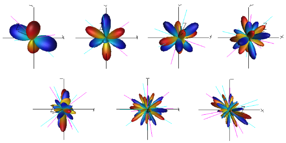
Figure 1: An image of the sky as decomposed into the $\ell=2$ through $8$ multipole moments based on the first year WMAP results wmap_results as cleaned by Tegmark et al. tegmark_cleaned . Shown are the $\sum_{m}a_{\ell m}Y_{\ell m}$ and the vectors calculated for these multipoles. The vectors are drawn as “sticks” since they only defined up to a sign (thus they are “headless” vectors). See http://www.phys.cwru.edu/projects/mpvectors/ for a full sized color picture.

III.2 Alternative derivation of vectors

In practice we have implemented the procedure described above (appendix A) and solved the set of equations (15) for the analysis we have performed. A mathematically more sophisticated decomposition procedure that leads to the same set of vectors without the need to calculate the $b_{m^{\prime}}$ begins by recognizing that

$$f_{\ell}(\Omega) = F^{(\ell)}_{i_{1}\cdots i_{\ell}}\left[\hat{e}^{i_{1}}\hat{e}^{i_{2}}\cdots\hat{e}^{i_{\ell}}\right]\equiv F^{(\ell)}_{i_{1}\cdots i_{\ell}}{\cal O}^{i_{1}\cdots i_{\ell}}$$

$$= A^{(\ell)}\left[\hat{v}^{(\ell,1)}_{i_{1}}\hat{v}^{(\ell,2)}_{i_{2}}\cdots\hat{v}^{(\ell,\ell)}_{i_{\ell}}\right]\left[\hat{e}^{i_{1}}\hat{e}^{i_{2}}\cdots\hat{e}^{i_{\ell}}\right].$$

Here $\hat{e}$ is again a radial unit vector, there is an implicit sum over repeated indices ($i_{1},\cdots,i_{\ell}$), and the square brackets represent the symmetric trace free part of the outer product. For a general symmetric tensor, $S^{(i_{1}\cdots i_{\ell})}=S^{i_{1}\cdots i_{\ell}}$,

$$\left[S^{i_{1}...i_{\ell}}\right] \equiv \frac{(\ell!)^{2}}{(2\ell)!}\sum_{k=0}^{\lfloor\ell/2\rfloor}(-1)^{k}\frac{(2\ell-2k)!}{k!(\ell-k)!(\ell-2k)!}$$

$$\times \delta^{(i_{1}i_{2}}\cdots\delta^{i_{2k-1}i_{2k}}S^{i_{2k+1}\cdots i_{\ell})p_{1}\cdots p_{2k}}$$

$$\times \delta_{p_{1}p_{2}}\cdots\delta_{p_{2k-1}p_{2k}},$$

where there is an implicit sum over the repeated indices $p_{1},...,p_{2k}$, and $()$ denotes symmetrization of the enclosed indices :

$$T^{(i_{1}\cdots i_{\ell})}\equiv\frac{1}{\ell!}\sum_{\pi\in U_{\ell}}T^{i_{\pi(1)}\cdots i_{\pi(\ell)}}.$$ (18)

($U_{\ell}$ is the group of permutations of the numbers $1,...,\ell$.) The particular combination

$${\cal O}^{i_{1}\cdots i_{\ell}}\equiv\left[\hat{e}^{i_{1}}\hat{e}^{i_{2}}\cdots\hat{e}^{i_{\ell}}\right]$$ (19)

simplifies considerably because $\hat{e}^{a}\hat{e}^{b}\delta_{ab}=1$

$${\cal O}^{i_{1}\cdots i_{\ell}} = \frac{(\ell!)^{2}}{(2\ell)!}\sum_{k=0}^{\lfloor\ell/2\rfloor}\left[(-1)^{k}\frac{(2\ell-2k)!}{k!(\ell-k)!(\ell-2k)!}\right.$$ (20)

$$\times\left.\delta^{(i_{1}i_{2}}\cdots\delta^{i_{2k-1}i_{2k}}\hat{e}^{i_{2k+1}}\cdots\hat{e}^{i_{\ell})}\right].$$

More importantly, it is easily calculable because of the recursion relation:

$$\left[\hat{e}^{i_{1}}\cdots\hat{e}^{i_{(j+1)}}\right]=\left[\hat{e}^{i_{1}}\left[\hat{e}^{i_{2}}\cdots\hat{e}^{i_{(j+1)}}\right]\right]$$ (21)

Similarly, the individual $\hat{v}^{(\ell,i)}$, can be peeled off one by one by recursion:

$$F^{(\ell)}_{i_{1}\cdots i_{\ell}} = \left[\hat{v}^{(\ell,1)}_{i_{1}},a^{(\ell,1)}_{i_{2}\cdots i_{\ell}}\right]$$

$$= \left[\hat{v}^{(\ell,1)}_{i_{1}},\left[\hat{v}^{(\ell,2)}_{i_{2}},a^{(\ell,2)}_{i_{3}\cdots i_{\ell}}\right]\right]$$

$$= A^{(\ell)}\left[\hat{v}^{(\ell,1)}_{i_{1}}\hat{v}^{(\ell,2)}_{i_{2}}\cdots\hat{v}^{(\ell,\ell)}_{i_{\ell}}\right]$$

assuming that the $F^{(\ell)}_{i_{1}\cdots i_{\ell}}$ can be calculated. But, these are easily represented as integrals over the sky (just as are the $a_{\ell m}$):

$$F^{(\ell)}_{i_{1}\cdots i_{\ell}}=\frac{(2\ell+1)(2\ell)!}{(4\pi)2^{\ell}(\ell!)^{2}}\int_{S_{2}}\frac{\Delta T(\Omega)}{T}{\cal O}^{i_{1}\cdots i_{\ell}}d\Omega$$ (23)

Alternatively, there is an explicit (analytic) relation between the $Y_{\ell m}$ and the $O^{i_{1}\cdots i_{\ell}}$, so that $F^{(\ell)}_{i_{1}\cdots i_{\ell}}$ can be expressed in terms of $a_{\ell m}$. Thus, given $F^{(\ell)}$ calculated from the sky, equation (III.2) is a sequence of $2\ell+1$ coupled quadratic equations for the $\hat{v}^{(\ell,i)}$ (and $A^{(\ell)}$) analogous to equation (13), in which the $b^{(\ell,i)}$ have been eliminated.

IV Sources of Error and Accuracy in Determining the Multipole Vectors

With the actual full-sky CMB maps, such as those that we use, the main source of error is pixel noise which accounts for the imperfections in measured temperature on the sky. Pixel noise depends on a variety of factors, one of which is the number of times a given patch has been observed. Pixel noise for WMAP is reported as $\sigma_{\rm pix}=\sigma_{0}/\sqrt{N_{\rm obs}}$, where $\sigma_{0}$ is noise per observation and $N_{\rm obs}$ is the number of observations per given pixel wmap_suppl . For the WMAP V-band map the reported noise per pixel is $\sigma_{0}=3.11\;{\rm mK}$ and the variation in the number of observations of each pixel is moderately small. Nevertheless, it is important to account for the inhomogeneous distribution of pixel noise, as we do in our full analysis in Secs. V and VI (where we find that the inhomogeneity of the pixel noise does not significantly change the main results). For the purposes of illustrating the accuracy in determining the multipole vectors, however, we assume a homogeneous noise with the measured mean value of $N_{\rm obs}=490$ observations per pixel.

The calculation of the pixel noise is straightforward. For equal-area pixels (as in Healpix healpix ) subtending a solid angle $\hat{\Omega}_{\rm pix}$ and assuming a full-sky map we have

$$a_{\ell m} = \int d\Omega\,Y_{\ell m}^{*}(\Omega)\,\Delta T(\Omega)$$ (24)

$$= \hat{\Omega}_{\rm pix}\sum_{\hat{\Omega}}Y_{\ell m}^{*}(\hat{\Omega})\,\Delta T(\hat{\Omega})$$

so that, using $\sigma_{\rm pix}^{2}\equiv\left\langle\left(\Delta T(\hat{\Omega})\right)^{2}\right\rangle\approx{\rm constant}$, we have

$$\langle a_{\ell m}a_{\ell^{\prime}m^{\prime}}^{*}\rangle$$ (25)

$$= \sum_{\hat{\Omega}}\hat{\Omega}_{\rm pix}Y_{\ell m}^{*}(\hat{\Omega})\sum_{\hat{\Omega}^{\prime}}\hat{\Omega}_{\rm pix}Y_{\ell^{\prime}m^{\prime}}(\hat{\Omega}^{\prime})\left\langle\Delta T(\hat{\Omega})\Delta T^{*}(\hat{\Omega}^{\prime})\right\rangle$$

$$= \hat{\Omega}_{\rm pix}\sum_{\hat{\Omega}}\hat{\Omega}_{\rm pix}Y_{\ell m}^{*}(\hat{\Omega})Y_{\ell m}^{*}(\hat{\Omega})\left\langle\left(\Delta T(\hat{\Omega})\right)^{2}\right\rangle\,\delta_{\ell\ell^{\prime}}\delta_{mm^{\prime}}$$

$$\simeq \hat{\Omega}_{\rm pix}\sigma_{\rm pix}^{2}\,\delta_{\ell\ell^{\prime}}\delta_{mm^{\prime}}.$$

Using the V-band map parameters, the pixel noise for NSIDE=512 Healpix resolution is $\sqrt{\hat{\Omega}_{\rm pix}}\,\sigma_{\rm pix}=2.7\times 10^{-4}$ mK. We adopt this quantity as an estimate of pixel noise for all maps we use.

IV.1 Accuracy in Determining the Multipole Vectors

We would like to find how accurately the multipole vectors are determined. To do this, we add a Gaussian-distributed noise with standard deviation $\sigma_{a_{\ell m}}$ to each $a_{\ell m}$

$$a_{\ell m}\rightarrow a_{\ell m}+\mathcal{N}(0,\sigma^{2}_{a_{\ell m}})$$ (26)

where $\mathcal{N}(\mu,\sigma^{2})$ denotes a Gaussian random variate with mean $\mu$ and variance $\sigma^{2}$. We repeat this many times in order to determine the distribution in the noise-added multipole vectors and their spherical coordinates $(\theta,\phi)$.

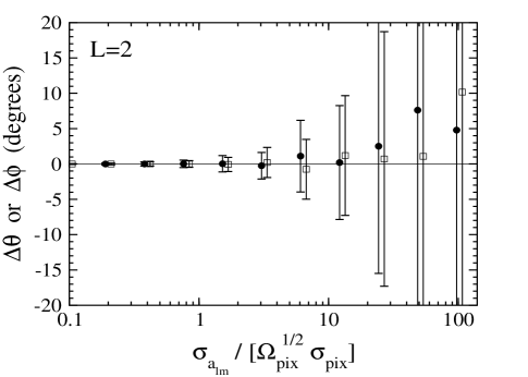
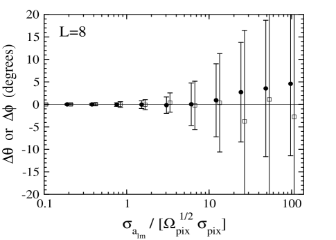
Figure 2: The accuracy in $\theta$ (filled circles) and $\phi$ (empty squares) of a chosen multipole vector as a function of noise added to the $a_{\ell m}$. Both the mean value and scatter in the shift of the angles are shown. The $x$-axis value of unity corresponds to the scatter in the $a_{\ell m}$ due to WMAP V-band pixel noise.

The mean and standard deviations of $\theta$ and $\phi$, as a function of $\sigma_{a_{\ell m}}$ (which is in units of WMAP V-band pixel noise $\sqrt{\hat{\Omega}_{\rm pix}}\,\sigma_{\rm pix}$) are shown in Fig. 2. The two panels show the effects on the $\ell=2$ and $\ell=8$ vectors. Note that both bias and scatter in $\theta$ and $\phi$ can be read off this figure. It is clear that the vectors are not extremely sensitive to the accuracy in the $a_{\ell m}$, and are determined to about $\pm 1$ degree for noise which is of order pixel noise. If the noise is much larger, however ($\sigma_{a_{\ell m}}\gtrsim 10\sqrt{\hat{\Omega}_{\rm pix}}\,\sigma_{\rm pix}$), the accuracy in multipole vectors deteriorates to the point that they are probably not useful as a representation of the CMB anisotropy. Accurate determination of $\theta$ and $\phi$ is expected to be especially important for higher multipoles, where the number of vectors is large.

V Tests of Non-Gaussianity With Multipole Vectors

Now that we have developed a formalism to compute the multipole vectors, we would like to test the WMAP map for any unusual features. Clearly, there doesn’t exist a test that simply checks for the “weirdness” of any particular representation of the map, in this case the multipole vectors. We can only test for features that we specify in advance. Here our general goal is to test the statistical isotropy of the map and search for any preferred directions.

Our motivation to devise and apply tests of statistical isotropy comes from findings that the quadrupole and octupole moments of WMAP maps lie in the plane of the Galaxy as discussed previously. One could in principle extend this and ask whether any higher multipoles lie preferentially in this (or any other) plane, and devise a statistic to test for this alignment. Clearly, the number of tests one can devise is very large. Here we would like to be as general as possible, and choose tests that suit our multipole vector representation. We choose to consider the dot product of multipole vectors between two different multipoles as described below.

V.1 Vector Product Statistics

A dot product of two unit vectors is a natural measure of their closeness. One test we consider is dot products between all vectors from the multipole $\ell_{1}$ with those from the multipole $\ell_{2}$. Since our vectors are really “sticks” (i.e. each vector is determined only up to a flip $\hat{v}\rightarrow-\hat{v}$), we always use the absolute value of a dot product. Furthermore, motivated by the fact that the WMAP quadrupole and octupole are located in the same plane and that their axes of symmetry are only about 10^∘ of each other angelica , we also consider using the cross-products of multipole vectors of any given multipole: if the vectors of $\ell_{1}$ and $\ell_{2}$ lie in a preferred plane, their respective cross products are oriented near a common axis perpendicular to the plane. Dot products of these two cross products would then be near unity.

We generalize this argument and make the following four choices for our statistic, which we shall call $S$. For any two multipoles $\ell_{1}$ and $\ell_{2}$, we consider the following.

1. Dot products of multipole vectors $|\hat{v}^{\,(\ell_{1},i)}\cdot\hat{v}^{\,(\ell_{2},j)}|$, where $\ell_{1}\neq\ell_{2}$, $\hat{v}^{\,(\ell_{1},i)}$ is the $i^{\rm th}$ vector from the $\ell_{1}$ multipole, and $\hat{v}^{\,(\ell_{2},j)}$ is the $j^{\rm th}$ vector from the $\ell_{2}$ multipole. We call this statistic “vector-vector”. For a given $\ell_{1}$ and $\ell_{2}$, there are clearly $M=\ell_{1}\ell_{2}$ distinct products. This statistic tests the orientation of vectors.

2. Dot products $|\hat{v}^{\,(\ell_{1},i)}\cdot(\hat{v}^{\,(\ell_{2},j)}\times\hat{v}^{\,(\ell_{2},k)})|/|\hat{v}^{\,(\ell_{2},j)}\times\hat{v}^{\,(\ell_{2},k)})|$ where where $\hat{v}^{\,(\ell_{1},i)}$ comes from the $\ell_{1}$ multipole and $\hat{v}^{\,(\ell_{2},j)}$ and $\hat{v}^{\,(\ell_{2},k)}$ from the $\ell_{2}$ multipole. We call this statistic “vector-cross”. For a given $\ell_{1}$ and $\ell_{2}$ and $j\neq k$, there are $M=\ell_{1}\ell_{2}(\ell_{2}-1)/2$ distinct products. This statistic tests the orientation of a vector with a plane.

3. Dot products $|(\hat{v}^{\,(\ell_{1},i)}\times\hat{v}^{\,(\ell_{1},j)})\cdot(\hat{v}^{\,(\ell_{2},k)}\times\hat{v}^{\,(\ell_{2},m)})|/(|(\hat{v}^{\,(\ell_{1},i)}\times\hat{v}^{\,(\ell_{1},j)})|\,|(\hat{v}^{\,(\ell_{2},k)}\times\hat{v}^{\,(\ell_{2},m)})|)$ where $\hat{v}^{\,(\ell_{1},i)}$ and $\hat{v}^{\,(\ell_{1},j)}$ come from the $\ell_{1}$ multipole and $\hat{v}^{\,(\ell_{2},k)}$ and $\hat{v}^{\,(\ell_{2},m)}$ come from the $\ell_{2}$ multipole. We call this statistic “cross-cross”. For a given $\ell_{1}$ and $\ell_{2}$ and $i\neq j$ and and $k\neq m$, there are $M=\ell_{1}(\ell_{1}-1)\ell_{2}(\ell_{2}-1)/4$ distinct products. This statistic tests the orientation of planes.

4. Dot products $|(\hat{v}^{\,(\ell_{1},i)}\times\hat{v}^{\,(\ell_{1},j)})\cdot(\hat{v}^{\,(\ell_{2},k)}\times\hat{v}^{\,(\ell_{2},m)})|$ where $\hat{v}^{\,(\ell_{1},i)}$ and $\hat{v}^{\,(\ell_{1},j)}$ come from the $\ell_{1}$ multipole and $\hat{v}^{\,(\ell_{2},k)}$ and $\hat{v}^{\,(\ell_{2},m)}$ come from the $\ell_{2}$ multipole. We call this statistic “oriented area”. For a given $\ell_{1}$ and $\ell_{2}$ and $i\neq j$ and and $k\neq m$, there are $M=\ell_{1}(\ell_{1}-1)\ell_{2}(\ell_{2}-1)/4$ distinct products. This statistic tests the orientation of areas. Notice it is similar to the previous test but the cross products are unnormalized.

V.2 Rank-Order Statistic

Figure 3: A flowchart of the algorithm we apply in order to extract the likelihood of the statistic, $S$. The lower case bold faced letters, such as (a), refer to the itemized points in section V B where more information can be found about the step. Also, the (V C) and (VI) refer to the sections in the paper where the details of these boxes can be found.

Having computed the statistic in question, we would like to know the likelihood of this statistic given the hypothesis that the $a_{\ell m}$ are statistically isotropic. The most straightforward way, and possibly the only reliable way, to do this is by comparing to Monte Carlo (MC) realizations of the statistically isotropic and Gaussian random $a_{\ell m}$. To be explicit, we provide the algorithm for computing the rank-ordered likelihood, and also illustrate it in the flowchart Fig. 3.

(a)

For $\ell_{1}$ and $\ell_{2}$ fixed, a statistic $S$ will produce $M$ numbers (dot products). We will use $S$ to test the hypothesis that the multipole vectors come from a map that exhibits statistical isotropy and Gaussianity. Calculate the $M$ numbers for this statistic for the WMAP map.

(b)

To determine the expected distributions for these $M$ numbers we begin by generating 100,000 Monte Carlo Gaussian, isotropic maps; in other words, we draw the coefficients $a_{\ell m}$ by assuming $\left\langle a_{\ell m}a_{\ell^{\prime}m^{\prime}}^{*}\right\rangle=C_{\ell}\delta_{\ell\ell^{\prime}}\delta_{mm^{\prime}}$. We are assuming statistical isotropy and Gaussianity, and this is the hypothesis that we are testing. We add a realization of inhomogeneous pixel noise, consistent with WMAP’s V-band noise, to each MC map. For each MC realization, we then compute the multipole vectors for multipoles $\ell_{1}$ and $\ell_{2}$, and $M$ dot products of the statistic $S$. Because the vectors of any particular realization do not have an identity (e.g. we do not know which one is the “fifth vector of $\ell=8$ multipole”) and neither do the dot products, we rank-order the $M$ dot products. At the end we have $M$ histograms of the products, each having 100,000 elements.

(c)

We would like to know the likelihood of the $M$ products computed from a WMAP map. To compute it we use a likelihood ratio test, which in the case of a single dot product of vectors would be the height of the histogram for the value of the statistic $S$ corresponding to WMAP relative to the maximum height. Since we have $M$ histograms, the likelihood trivially generalizes to

$$\mathcal{L}_{\rm WMAP}=\prod_{j=1}^{M}\frac{N_{j,\rm WMAP}}{N_{j,\rm max}}$$ (27)

where $N_{j,\rm WMAP}$ is the ordinate of the $j^{\rm th}$ histogram corresponding to WMAP’s $j^{\rm th}$ rank-ordered product, $N_{j,\rm max}$ is the maximum value of $j^{\rm th}$ histogram, and the product runs over all $M$ histograms.

(d)

Now that we have the WMAP likelihood, we need to compare it to “typical” likelihoods produced by Monte Carlo realizations of the map. (An alternative approach, computing the expected distribution of the likelihood from first principles, would be much more difficult since one would have to explicitly take into account the correlations between $M$ products.) To do this, we generate another 50,000 Gaussian random realizations of coefficients $a_{\ell_{1}m}$ and $a_{\ell_{2}m}$, and compute the multipole vectors and the statistic $S$ for each realization.

(e)

We rank-order the likelihood $\mathcal{L}_{\rm WMAP}$ among the 50,000 likelihoods from MC maps to obtain its rank $R_{\ell_{1},\ell_{2}}$.

(f)

Finally we go to step (a) and repeat the whole procedure for all pairs of multipoles $(\ell_{1},\ell_{2})$ that we wish to test. Only when we have the complete set do we assign a probability.

The rank $R_{\ell_{1},\ell_{2}}$ gives the probability that the statistic $S_{\rm WMAP}$ is consistent with the test hypothesis. For example, if the likelihood of $S_{\rm WMAP}$ is rank $900$ out of $1000$, then there is a 10% probability that a Monte Carlo Gaussian random realization of the CMB sky will give higher likelihood, and 90% probability for a lower MC likelihood. We say that the rank order of this particular likelihood is 0.9. If our CMB sky is indeed random Gaussian, we would expect the rank-orders of our statistics to be distributed between 0 and 1, being neither too small nor too large. Conversely, if we computed the rank-orderings for three different multipoles for a particular test and obtained 0.98, 0.99 and 0.95, (or 0.01, 0.05 and 0.02, say), we would suspect that this particular test is not consistent with the Gaussian random hypothesis.

V.3 How unusual are the ranks?

We now consider how to quantify the confidence level for rejecting the hypothesis of statistical isotropy of the $a_{\ell m}$. Let us assume that we have computed the rank orders for $N$ different pairs of multipoles, and obtained the rank-orderings of $x_{i}$ for the $i^{\rm th}$ one, where $0\leq x_{i}\leq 1$. We consider the following parametric test.

The test anticipates that the ranks will be unusually high. Let us first order the ranks $x_{i}$ in descending order, so that $x_{1}$ is the largest and $x_{N}$ the smallest. We calculate the following statistic

$$Q(x_{1},\ldots,x_{N})=N!\int_{x_{1}}^{1}dy_{1}\,\int_{x_{2}}^{y_{1}}dy_{2}\ldots\int_{x_{N}}^{y_{N-1}}dy_{N}.$$ (28)

If the ranks $R_{\ell_{1},\ell_{2}}$ were expected to be uniformly distributed in $[0,1]$, $Q$ would be the probability that the highest rank is greater than $x_{1}$, and the second-biggest rank greater than $x_{2}$, …, and the smallest rank greater than $x_{N}$. However we do not expect that the ranks from Gaussian random maps are uniformly distributed, and we treat $Q$ merely as a statistic. We then ask that given the (possibly very small) value of $Q_{\rm WMAP}$, what fraction of Gaussian random maps would give an even smaller $Q$? That number is our probability, and is computed in the next section. Note that, although apparently difficult or impossible to evaluate analytically, the right-hand side of Eq. (28) can trivially be computed using a recursion relation as shown in appendix B.

VI Results

Table I shows the final ranks for the vector-vector, vector-cross, cross-cross, and oriented area tests for pairs ($\ell_{1},\ell_{2}$). These results correspond to the full-sky cleaned WMAP map from Tegmark et al. tegmark_cleaned (results for their Wiener-filtered map from the same reference are essentially identical). The ranks from the WMAP ILC full-sky map are similar, and to make the presentation concise we show the ILC map oriented area ranks in Table I, but otherwise only quote final probabilities for the ILC ranks. As discussed earlier, a detailed analysis of cut-sky maps will be presented in an upcoming publication.

For computational convenience we considered only the multipoles $2\leq\ell_{1},\ell_{2}\leq 8$; we discuss the upper multipole limit in section VI.3. Note that, for the vector-cross test, ($\ell_{1},\ell_{2}$) and ($\ell_{2},\ell_{1}$) products are distinct and both need to be considered.

Ranks of Products of Multipole Vectors
	Vector-Vector		Vector-Cross			Cross-Cross		Oriented Area		O. A. (ILC map)
($\ell_{1},\ell_{2}$)	$M$	Rank	$M$	($\ell_{1},\ell_{2}$) Rank	($\ell_{2},\ell_{1}$) Rank	$M$	Rank	$M$	Rank	$M$	Rank
(2, 3)	6	0.57714	6, 3	0.03176	0.04814	3	0.01316	3	0.00126	3	0.00886
(2, 4)	8	0.39167	12, 4	0.51983	0.20369	6	0.56747	6	0.96042	6	0.62279
(2, 5)	10	0.66656	20, 5	0.85252	0.10536	10	0.22285	10	0.71820	10	0.77484
(2, 6)	12	0.53649	30, 6	0.50367	0.67791	15	0.87882	15	0.76320	15	0.93862
(2, 7)	14	0.44925	42, 7	0.74254	0.52205	21	0.91890	21	0.86496	21	0.63763
(2, 8)	16	0.21683	56, 8	0.20861	0.73486	28	0.91338	28	0.68520	28	0.99986
(3, 4)	12	0.18093	18, 12	0.75272	0.30611	18	0.17059	18	0.34475	18	0.12562
(3, 5)	15	0.21511	30, 15	0.36963	0.78578	30	0.37187	30	0.67870	30	0.76284
(3, 6)	18	0.31507	45, 18	0.26683	0.54146	45	0.75052	45	0.93546	45	0.52839
(3, 7)	21	0.98772	63, 21	0.85874	0.57072	63	0.55147	63	0.73650	63	0.83324
(3, 8)	24	0.76120	84, 24	0.98578	0.60408	84	0.99988	84	0.99656	84	0.97766
(4, 5)	20	0.41209	40, 30	0.28221	0.84716	60	0.54035	60	0.52936	60	0.65965
(4, 6)	24	0.68840	60, 36	0.58372	0.86140	90	0.74826	90	0.62266	90	0.73762
(4, 7)	28	0.85008	84, 42	0.51404	0.95584	126	0.53715	126	0.88992	126	0.32153
(4, 8)	32	0.48723	112, 48	0.56328	0.85462	168	0.84374	168	0.99006	168	0.95266
(5, 6)	30	0.82148	75, 60	0.42361	0.88662	150	0.66327	150	0.82760	150	0.86242
(5, 7)	35	0.86884	105, 70	0.56542	0.96116	210	0.59483	210	0.68920	210	0.98440
(5, 8)	40	0.83380	140, 80	0.96812	0.34287	280	0.30403	280	0.24449	280	0.33959
(6, 7)	42	0.03742	126, 105	0.13831	0.02203	315	0.20221	315	0.97286	315	0.78414
(6, 8)	48	0.92760	168, 120	0.91468	0.78058	420	0.72850	420	0.62894	420	0.66873
(7, 8)	56	0.03238	196, 168	0.04440	0.02060	588	0.09552	588	0.25367	588	0.24871

Table 1: Ranks of the vector-vector, vector-cross, cross-cross, and oriented area statistics for multipoles $2\leq\ell_{1},\ell_{2}\leq 8$ for the four tests we consider as applied to the Tegmark et al. tegmark_cleaned cleaned map. Also listed are the oriented area ranks for the ILC map. $M$ is the number of products for a given statistic for each $(\ell_{1},\ell_{2})$ pair. In section VI.2 we perform a parametric test to compute the likelihood of oriented area ranks being this high.

VI.1 Vector-vector, vector-cross, and cross-cross ranks

Table I shows that the vector-vector ranks are distributed roughly as expected, nearly uniformly in the interval $[0,1]$. The vector-cross ranks, however, are starting to shows hints of an interesting feature that will be more pronounced later in the cross-cross and oriented area tests: ranks that are unusually high: seven ranks out of 42 are greater than 0.9. The probability of this happening, however, is not statistically significant and may be purely accidental.

The first big surprise comes from the cross-cross ranks: the $(\ell_{1}=3,\ell_{2}=8)$ rank is $0.99988$. This means that only 6 out of 50,000 MC generated maps had a higher likelihood than the WMAP map! In other words, the $84$ cross-cross dot products computed for this pair from WMAP lie unusually near the peaks of their respective histograms, which, recall, are built out of 100,000 products from MC map realizations. The violation of statistical isotropy and/or Gaussianity therefore manifests itself by a particular correlation between the vectors which makes the statistic $S_{\rm WMAP}$ “unusually usual”. Since we checked that the distribution of Monte-Carlo generated $(\ell_{1}=3,\ell_{2}=8)$ cross-cross ranks is uniform in the interval $[0,1]$, it is easy to see that the probability of this rank being this high (or higher) is $6/50,000$, or $0.012$%. Admittedly, we checked $21$ such cross-cross ranks, which raises the probability of find such a result to $0.26$%. If we include all vector-vector, vector-cross, cross-cross and oriented area ranks, the probability rises to a still rather low $1.3$%.

Note that this effect is very different from the now-familiar orientation of the quadrupole and octupole axes; the quadrupole-octupole alignment is quite unlikely and results in multipole vector products which preferentially fall on the tails of their respective histograms. This is confirmed by the actual ranks for ($2,3$) and ($3,2$) multipole vector-cross products, and also the ($2,3$) cross-cross and oriented area products, all of which are fairly low ($\lesssim 0.05$). This is easy to understand: in the cross-cross product case, for example, the fact that the multipole vectors lie mostly in the Galaxy plane implies that their cross products are roughly perpendicular to this plane. The dot products of those are then, by absolute value, very large, and hence unusual. What we are seeing here is that the $(\ell_{1}=3,\ell_{2}=8)$ cross-cross products from the WMAP full-sky map are unusually usual.

VI.2 Oriented area ranks

As mentioned above, one of the cross-cross ranks was extremely high. A much bigger surprise is found when we examine the oriented area ranks (see also Fig. 4): 2 (out of 21) are greater than 0.99, a total of 5 are greater than 0.9, and a total of 8 are greater than 0.8! These ranks are clearly not distributed in the same way as those from a typical MC map.

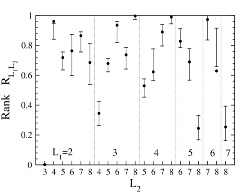
Figure 4: Ranks of the oriented area statistics for the Tegmark full-sky map. The mean values correspond to the actual extracted $a_{\ell m}$, while the error bars were obtained by adding the pixel noise (the error bars are not necessarily symmetric around the no-error values). Note that an unusually large fraction of the ranks are high. Also note the low value of $\ell_{1}=2$, $\ell_{2}=3$ rank which is due to the alignment of the quadrupole and octupole which has been noted earlier tegmark_cleaned .

To examine the probability of the ranks being this high we perform the parametric test described in section V.2 and in appendix B: we compute the statistic $Q$ which, for a distribution of ranks expected to be uniform in $[0,1]$, would be the probability of the largest one being at least as large as the largest actual WMAP rank and the second largest being at least as large as the second-largest actual rank, etc. This statistic, applied to ranks from the Tegmark et al. cleaned map, is

$$Q=10^{-(6.12^{+0.62}_{-1.16})}$$ (29)

where the error around the mean value is estimated by repeatedly adding the pixel noise of the map to the pure extracted $a_{\ell m}$, as in Eq. (26), and estimating the effect on the products of multipole vectors and their ranks.

However, we have to be cautious not to over-interpret $Q$ as the final probability—it has to be compared to Monte Carlo probabilities computed under the same conditions to determine its distribution. To this end, we generate 10,000 additional MC Gaussian random maps and compute $Q$ for each. It turns out that only 107 of them produce $Q$ lower than the WMAP value in (29). This is further illustrated in Fig. 5, which also shows the error bars on the WMAP $Q$. The probability of WMAP oriented area ranks being this high, according to the $Q$-test, is 1.07%, which corresponds to a 2.6-$\sigma$ (or $98.93\%$) evidence for the violation of statistical isotropy and/or Gaussianity. The connection of this (nearly) 3-$\sigma$ deviation to the nearly 3-$\sigma$ deviation represented by the $(\ell_{1}=3,\ell_{2}=8)$ cross-cross rank remains somewhat unclear.

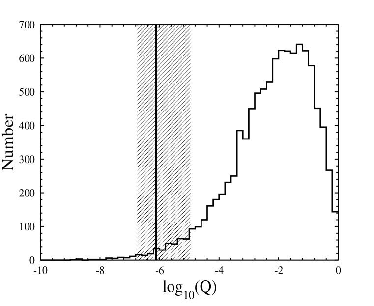
Figure 5: The statistic $Q$ for the oriented area statistic, computed from the Tegmark et al. cleaned WMAP map, is shown by vertical line. The shaded region around it corresponds to the uncertainty due to pixel noise, while the histogram shows the distribution of the statistic for MC-generated Gaussian maps. Only $1.07\%$ of MC values of $Q$ are smaller than the no-error value of the WMAP $Q$. The same fraction for the ILC map (not shown here) is $0.38\%$.

VI.3 Further tests

We have performed a few tests to explore the stability of the oriented area result. First, we have varied the multipole range from the fiducial $2\leq\ell\leq 8$; the results are shown in Table II. Increasing the lower limit, $\ell_{\rm min}$, leads to the final probability of $1\%$ and $5.6\%$ for $\ell_{\rm min}=3$ and 4 respectively. Therefore, evidence for the violation of statistical isotropy weakens, but does so relatively slowly. This shows that our main result does not completely hinge on the quadrupole and octupole. Same can be said for the upper multipole limit, which gives strongest results for the violation of statistical isotropy with $\ell_{\rm max}=8$, but with decreasing $\ell_{\rm max}$ the result does not immediately go away. Finally, we have checked that increasing $\ell_{\rm max}$ to higher values, up to 12, does not produce new ranks that are unusually high. The correlations are therefore most apparent in the multipole range $2\leq(\ell_{1},\ell_{2})\leq 8$.

Varying the Multipole Coverage
$\ell_{\rm min}$	$Q_{\rm WMAP}$	$f(Q_{\rm MC}<Q_{\rm WMAP})$
2	$7.61\times 10^{-7}$	$107/10000$
3	$3.13\times 10^{-6}$	$105/10000$
4	$3.12\times 10^{-4}$	$565/10000$
$\ell_{\rm max}$	$Q_{\rm WMAP}$	$f(Q_{\rm MC}<Q_{\rm WMAP})$
8	$7.61\times 10^{-7}$	$107/10000$
7	$3.72\times 10^{-5}$	$394/10000$
6	$3.62\times 10^{-3}$	$2079/10000$

Table 2: Final probabilities of the WMAP oriented area statistic as a function of multipole coverage $l_{\rm min}\leq l\leq l_{\rm max}$. The fiducial case is $2\leq\ell\leq 8$ and we have shown how the results change if the lower and upper bounds are changed. $f(Q_{\rm MC}<Q_{\rm WMAP})$ is the fraction of MC random Gaussian maps that give a value of $Q$ smaller than WMAP.

We next check if the correlations can be explained by any remaining dust contamination. We use WMAP’s V-band map of the identified thermal dust; this map was created by fitting to the template model from Ref. finkbeiner . We assume for a moment that 10% of the identified contamination by dust had not been accounted for, and we add it to the cleaned CMB map, i.e. $T_{\rm tot}=T_{\rm CMB}+0.1\,T_{\rm dust}$. Although we are adding a significant contamination (the remaining dust is expected to contribute no more than a few percent to the rms CMB temperature wmap_results ), the high oriented area ranks do not change much (they actually slightly increase), and the Gaussian isotropic hypothesis is still ruled out at the 99.3% level. Clearly, dust contamination does not explain our results. Further, to mimic remaining foregrounds due to an imperfect cleaning of the map we tested adding a synthetic random Gaussian map which contributed 10% of the RMS temperature. We find that the oriented area statistic still disagrees with the Gaussian isotropic hypothesis at the 99.4% level.

Finally, we have repeated the analysis with several other available full-sky CMB maps. As mentioned earlier, both maps analyzed by Tegmark et al. give the same probability for the oriented area statistic. For the WMAP ILC map we find similarly high ranks, giving an even smaller value for our statistic: $Q_{\rm ILC}=2.44\times 10^{-7}$, and only 62 MC maps out of 10000 have a smaller value of $Q$; therefore, the high ranks in the ILC map are unlikely at the 99.38% level, corresponding to 2.7-$\sigma$.

VII Discussion

Does the apparent violation of statistical isotropy or Gaussianity that we detected have a cosmological origin, or is it due to foregrounds or measurement error? The results presented in this paper refer to full-sky maps, and it is known that there are two large cold and two hot spots in the Galaxy plane, and that any result that depends on structure in this plane is suspect. Nevertheless, it is far from obvious that the result is caused by the contamination in the map for the following reasons:

• As Tegmark et al. tegmark_cleaned argue, their cleaned map agrees very well with the ILC map on large scales, although the two were computed using different methods. The results we presented indicate a violation of isotropy and/or Gaussianity at $\geq 98.9\%$ confidence using either map. Furthermore, instrumental noise and beam uncertainties are completely subdominant on these scales.

• The results come from an effect different than the quadrupole and octupole alignment: the latter is fairly unlikely, as discussed in Ref. angelica , while we see a particular correlation between the vectors that makes our statistic $S$ unusually likely.

• Perhaps most importantly, our results are mostly (though not completely) independent of the quadrupole and octupole, multipoles that might be suspect. For example, the second-highest oriented area rank is $(\ell_{1}=4,\ell_{2}=8)$. Furthermore, Table 2 shows that if we only use the multipoles $4\leq\ell_{1},\ell_{2}\leq 8$, the oriented area statistic still rules out the Gaussian random hypothesis at the $94.4\%$ level.

At this time it is impossible to ascertain the origin of the additional correlation between the multipole vectors that we are seeing. One obvious way to find out more about their origin is to Monte Carlo generate maps that are non-Gaussian or violate the statistical isotropy, according to a chosen prescription, and see whether our statistics, $S_{\rm WMAP}$, agree with the $S$ computed from MC maps. Of course, there are many different ways in which Gaussianity and/or isotropy can be broken, and there is no guarantee that we can find one that explains our results.

Another possibility is to cut the galaxy (or other possible contaminations) from the map prior to performing the vector decomposition. There are two approaches we can take: (1) use the cut-sky $a_{\ell m}$ to compute the multipole vectors and the statistics $S$ and compare those to $S$ computed from cut-sky Gaussian random maps, or (2) reconstruct the true full-sky $a_{\ell m}$ and compare with full-sky Gaussian random maps. The latter procedure is preferred as one would like to work with the true multipole vectors of our universe, but reconstructing the full-sky map from the cut-sky information is a subtle problem that will introduce an additional source of error. Nevertheless, the total error with a $\sim 10^{\circ}$ cut may still be small enough to allow using the vectors as a potent tool for finding any preferred directions in the universe. We are actively pursuing these approaches at the present time.

Finally, Park park recently tested the full-sky WMAP maps using the genus statistic and found evidence for the violation of Gaussianity at 2–3$\,\sigma$ level, depending on the smoothing scale and the chosen aspect of the statistic. Furthermore Eriksen et al. NorthSouth find that the WMAP multipoles with $\ell<35$ have significantly less power in the northern hemisphere than in the southern hemisphere. It is possible that these results and the effects discussed in this paper have the same underlying cause, but this cannot be confirmed without further tests.

VIII Conclusions

The traditional $Y_{\ell m}$ expansion of the sky has many advantages. For one, each set of $Y_{\ell m}$ of fixed $\ell$ form an irreducible representation of the rotation group in three dimensions $O(3)$; for another, more than two centuries of effort have lead to a rich mathematical literature on the $Y_{\ell m}$, their properties, and how to efficiently calculate them. The coefficients, $a_{\ell m}$ of a $Y_{\ell m}$ expansion of a function on the sphere are readily calculated as integrals over the sphere of the function times the $Y_{\ell m}^{*}$. In this paper we have considered a different basis of an equivalent irreducible representations of the proper rotation group, ${\cal O}_{(\ell)}^{i_{1}\cdots i_{\ell}}$ – for each $\ell$, the traceless symmetric product of $\ell$ copies of the unit vector of coordinates ${\hat{e}}(\Omega)$. These are merely linear combinations of the $Y_{\ell m}$, and so share many of the properties of them, albeit with a more sparse mathematical literature explicitly dedicated to their properties. In particular the coefficients $F^{(\ell)}_{i_{1}\cdots i_{\ell}}$ of a ${\cal O}_{(\ell)}$ expansion of a function on the sky are, like the spherical harmonic coefficients, calculable as integrals over the sphere of the function times ${\cal O}_{(\ell)}$.

We have expressed the $F^{(\ell)}_{i_{1}\cdots i_{\ell}}$ as symmetric traceless products of $\ell$ (headless) unit vectors $\{\hat{v}^{(\ell,i)}\}$ and a scalar $A^{(\ell)}$. The $\{\hat{v}^{(\ell,i)}\}$ are highly non-linear functions of the $a_{\ell m}$. Thus, while in principle they encode the exact same information, they may make certain features of the data more self-evident. In particular we claim that these “multipole vectors” are natural sets of directions to associate with each multipole of the sky. A code to calculate multiple vectors from CMB skies is available on our website at http://www.phys.cwru.edu/projects/mpvectors/.

We have obtained the multipole vectors of the CMB sky as measured by WMAP, as well as the oriented areas defined by all pairs of such vectors (within a particular multipole). We have examined the hypothesis that the vectors of multipole $\ell$ are uncorrelated with the vectors of multipole $\ell^{\prime}$ for $\ell$ and $\ell^{\prime}$ up to 8. We have done this by comparing in turn the dot products of the vectors from $\ell$ with those from $\ell^{\prime}$, the dots products of the vectors with the unit normals to the planes. the dot products of the unit normals to the planes with each other, and the dot products of the normals to the planes with each other, We have found that while there is nothing unusual about the distribution of dot products of the vectors with each other, the dot products of the normals to the planes with each other (and, to a lesser extent, the dot products of the unit normals to the planes with each other) are inconsistent with the standard assumptions of statistical isotropy and Gaussianity of the $a_{\ell m}$. To quantify this inconsistency we compared the distribution of these dot products with those from $50,000$ Monte Carlo simulations and found that they are inconsistent at the level of 107 parts in 10000 for the Tegmark et al. cleaned full-sky map and 62 parts in 10000 for the ILC full-sky map. These results are robust to the inclusion of appropriate Poisson noise. The sensitivity to a Galactic cut will be explored in a future publication, but preliminary results suggest that the results persist within the error bars, but eventually decline in statistical significance as the uncertainties increase with increasing cuts.

Appendix A Vector decomposition equations

The vector decomposition equations we derived (15) can be recast in a numerically more convenient form. The equations, as written, involve complex valued coefficients. Here we rewrite these equations in terms of their purely real components. To begin we note that the spherical harmonics satisfy $Y_{\ell,-m}(\Omega)=(-1)^{m}Y_{\ell m}^{*}(\Omega)$. Thus the decomposition coefficients of a real valued function, such as $\Delta T(\Omega)/T$, satisfy $a_{\ell,-m}^{*}=(-1)^{m}a_{\ell m}$. This shows that all the information about the function is encoded in the real part of $a_{\ell 0}$ (the imaginary part is identically zero) and the real and imaginary parts of $a_{\ell m}$ for $1\leq m\leq\ell$. These are the $2\ell+1$ independent components we use in the vector decomposition. We thus only need to solve (15) for $0\leq m\leq\ell$.

For notational convenience we drop the $(\ell)$ superscript on $a_{\ell-1,m-j}$, $b_{m^{\prime}}$, and $\hat{v}$. It should be understood that these quantities are associated with a particular multipole and step in the recursive decomposition procedure as outlined in section III.1. The correspondence between the dipole and Cartesian coordinate directions (7) allows us to identify $\hat{v}=(\hat{v}_{-1},\hat{v}_{0},\hat{v}_{1})$ with standard coordinate axes via

$$\hat{v}_{-1} = \frac{1}{\sqrt{2}}\left(\hat{v}_{x}+i\hat{v}_{y}\right),$$

$$\hat{v}_{0} = \hat{v}_{z},$$ (30)

$$\hat{v}_{1} = -\frac{1}{\sqrt{2}}\left(\hat{v}_{x}-i\hat{v}_{y}\right).$$

Finally the real and imaginary parts of the $a_{\ell m}$ are

$$a_{\ell m}^{\rm re}=\frac{1}{2}\left(a_{\ell m}+a_{\ell m}^{*}\right)\quad\hbox{and}\quad a_{\ell m}^{\rm im}=\frac{1}{2i}\left(a_{\ell m}-a_{\ell m}^{*}\right).$$ (31)

Applying (30) and (31) to the multipole vector decomposition equations (15) gives the following equations

$$a_{\ell m}^{\rm re} = C_{0}^{(l,m)}a_{\ell-1,m}^{\rm re}\hat{v}_{z}+\frac{1}{\sqrt{2}}C_{-1}^{(\ell,m)}\left(a_{\ell-1,m+1}^{\rm re}\hat{v}_{x}-a_{\ell-1,m+1}^{\rm im}\hat{v}_{y}\right)-\frac{1}{\sqrt{2}}C_{1}^{(\ell,m)}\left(a_{\ell-1,m-1}^{\rm re}\hat{v}_{x}+a_{\ell-1,m-1}^{\rm im}\hat{v}_{y}\right),$$

$$a_{\ell m}^{\rm im} = C_{0}^{(l,m)}a_{\ell-1,m}^{\rm im}\hat{v}_{z}+\frac{1}{\sqrt{2}}C_{-1}^{(\ell,m)}\left(a_{\ell-1,m+1}^{\rm im}\hat{v}_{x}+a_{\ell-1,m+1}^{\rm re}\hat{v}_{y}\right)-\frac{1}{\sqrt{2}}C_{1}^{(\ell,m)}\left(a_{\ell-1,m-1}^{\rm im}\hat{v}_{x}-a_{\ell-1,m-1}^{\rm re}\hat{v}_{y}\right),$$

$$a_{\ell 0}=a_{\ell 0}^{\rm re} = C_{0}^{(l,0)}a_{\ell-1,0}^{\rm re}\hat{v}_{z}+\sqrt{2}C_{1}^{(\ell,0)}\left(a_{\ell-1,1}^{\rm re}\hat{v}_{x}-a_{\ell-1,1}^{\rm im}\hat{v}_{y}\right),$$ (32)

$$b_{m^{\prime}}^{\rm re} = D_{0}^{(l,m)}a_{\ell-1,m}^{\rm re}\hat{v}_{z}+\frac{1}{\sqrt{2}}D_{-1}^{(\ell,m)}\left(a_{\ell-1,m+1}^{\rm re}\hat{v}_{x}-a_{\ell-1,m+1}^{\rm im}\hat{v}_{y}\right)-\frac{1}{\sqrt{2}}D_{1}^{(\ell,m)}\left(a_{\ell-1,m-1}^{\rm re}\hat{v}_{x}+a_{\ell-1,m-1}^{\rm im}\hat{v}_{y}\right),$$

$$b_{m^{\prime}}^{\rm im} = D_{0}^{(l,m)}a_{\ell-1,m}^{\rm im}\hat{v}_{z}+\frac{1}{\sqrt{2}}D_{-1}^{(\ell,m)}\left(a_{\ell-1,m+1}^{\rm im}\hat{v}_{x}+a_{\ell-1,m+1}^{\rm re}\hat{v}_{y}\right)-\frac{1}{\sqrt{2}}D_{1}^{(\ell,m)}\left(a_{\ell-1,m-1}^{\rm im}\hat{v}_{x}-a_{\ell-1,m-1}^{\rm re}\hat{v}_{y}\right),$$

$$b_{0}=b_{0}^{\rm re} = D_{0}^{(l,0)}a_{\ell-1,0}^{\rm re}\hat{v}_{z}+\sqrt{2}D_{1}^{(\ell,0)}\left(a_{\ell-1,1}^{\rm re}\hat{v}_{x}-a_{\ell-1,1}^{\rm im}\hat{v}_{y}\right),$$

$$|\hat{v}| = \hat{v}_{x}^{2}+\hat{v}_{y}^{2}+\hat{v}_{z}^{2}=1.$$

Note that the equations for the $b_{m^{\prime}}$ are identical to those for $a_{\ell m}$ with $D^{(\ell,m)}$ inserted in place of $C^{(\ell,m)}$. Here $1\leq m\leq\ell$ and $1\leq m^{\prime}\leq\ell-2$. These equations involve only real quantities and can thus be easily coded and solved. These are the equations we have implemented to find the multipole vectors.

Appendix B Probability of rank orderings

Consider $N$ numbers $x_{i}$, where $0\leq x_{i}\leq 1$, and order them in descending order, so that $x_{1}$ is the largest and $x_{N}$ the smallest. Let us then consider a set of variates $y_{i}$ uniformly distributed in the interval $[0,1]$, and also order them in descending order so that $y_{1}$ is the largest one and $y_{N}$ the smallest. We ask: what is the probability that $y_{1}$ is greater than $x_{1}$, and that $y_{2}$ is greater than $x_{2}$, …, and the $y_{N}$ is greater than $x_{N}$.

The probability that $y_{1}$ is in the interval $[x_{1},x_{1}+dx_{1}]$, $\mathcal{P}_{1}(x_{1})dx_{1}$, is

$$\mathcal{P}_{1}(x_{1})dx_{1}={N\choose 1}x_{1}^{N-1}dx_{1}$$ (33)

and the probability that $y_{1}$ is larger than $x_{1}$, $P_{1}(x_{1})$, is obviously

$$P_{1}(x_{1})=\int_{x_{1}}^{1}\mathcal{P}_{1}(y_{1})dy_{1}.$$ (34)

Given that $y_{1}$ is greater than $x_{1}$, the probability that the $y_{2}$ is in the interval $[x_{2},x_{2}+dx_{2}]$

$$\mathcal{P}_{2}(x_{2}|x_{1})dx_{2}={N-1\choose 1}\,\left(\frac{x_{2}}{x_{1}}\right)^{N-2}\,\frac{dx_{2}}{x_{1}}$$ (35)

and the probability that the largest $y$ is greater than $x_{1}$ and the second-largest greater than $x_{2}$ is

$$P_{2}(x_{1},x_{2}) = \int_{x_{1}}^{1}\mathcal{P}_{1}(y_{1})dy_{1}\int_{x_{2}}^{y_{1}}\mathcal{P}_{2}(y_{2}|y_{1})dy_{2}$$ (36)

$$= N(N-1)\int_{x_{1}}^{1}dy_{1}\int_{x_{2}}^{y_{1}}y_{2}^{N-2}dy_{2}.$$

We can continue this argument for all other $y_{i}$ and $x_{i}$, in descending order in $x_{i}$. The final probability, the joint probability of $i^{\rm th}$ largest $y$ being greater than $x_{i}$ for all $i$, is given by

$$P_{N}(x_{1},x_{2},\ldots,x_{N})=N!\int_{x_{1}}^{1}dy_{1}\int_{x_{2}}^{y_{1}}dy_{2}\ldots\int_{x_{N-1}}^{y_{N-1}}dy_{N}.$$ (37)

We would like to evaluate this integral. Even though the result will obviously be a polynomial in $x_{i}$, there is a total of $2^{N}$ terms and it is difficult to do the bookkeeping. However, there is a simple recursion formula for this integral. Assume, more generally, that we want to compute

$$I_{N}^{\alpha}\equiv\int_{x_{1}}^{1}dy_{1}\int_{x_{2}}^{y_{1}}dy_{2}\ldots\int_{x_{N-1}}^{y_{N}}dy_{N}\,y_{N}^{\alpha}.$$ (38)

One can then perform the innermost integral, and this leads to the recursion relation

$$I_{N}^{\alpha}=\frac{1}{\alpha+1}\,\left[I_{N-1}^{\alpha+1}-x_{N}^{\alpha+1}I_{N-1}^{0}\right].$$ (39)

We are left with two $(N-1)$-tuple integrals. Therefore, starting from the $N$-dimensional integral, we can recursively bring it down all the way to $N=1$, at which point it is an easy one-dimensional integral

$$I_{1}^{\beta}\equiv\int_{x_{1}}^{1}dy_{1}\,y_{1}^{\beta}=\frac{1}{\beta+1}\left[1-x_{1}^{\beta+1}\right].$$ (40)

for the required $\beta$. Using the recursion relation (39), together with (40), we numerically compute the probability in (37).

References

- (1) C.L. Bennett et.al., Astrophys. J. 148, S1 (2003)
- (2) C.L. Bennett et.al., Astrophys. J. 148, S97 (2003)
- (3) G. Hinshaw et.al., Astrophys. J. 148, S135 (2003)
- (4) D.N. Spergel et al., Astrophys. J. 148, S175 (2003)
- (5) S. Hanany et al., Astrophys. J. 545, L5 (2000)
- (6) N.W. Halverson et al., Astrophys. J. 568, 38 (2002)
- (7) C.L. Kuo et al., Astrophys. J. 600, 32 (2004)
- (8) T.J. Pearson et al., Astrophys. J. 591, 556 (2003)
- (9) A.C. Taylor et al., Mon. Not. R. Astron. Soc. 341, 1066 (2003)
- (10) A. Benoit et al., Astron. Astrophys. 399, L19 (2003)
- (11) J.E. Ruhl et al., Astrophys. J. 599, 786 (2003)
- (12) E.F. Bunn and D. Scott, Mon. Not. R. Astron. Soc. 331, 313 (2000)
- (13) M. Tegmark, A. de Oliveira-Costa and A.J.S. Hamilton, Phys. Rev. D, 68, 123523 (2003)
- (14) H.K. Eriksen, F.K. Hansen, A.J. Banday, K.M. Gorski, and P.B. Lilje., submitted (astro-ph/0307507)
- (15) C.-G. Park, Mon. Not. R. Astron. Soc., 349, 313 (2004)
- (16) A. Hajian, T. Souradeep, N. Cornish, D.N. Spergel, and G.D. Starkman, in preparation
- (17) A. Hajian and T. Souradeep, submitted to PRL (astro-ph/0301590)
- (18) P. Vielva, E. Martinez-Gonzalez, R.B. Barreiro, J.L. Sanz and L. Cayon, astro-ph/0310273
- (19) F.R. Bouchet, D.P. Bennett and A. Stebbins, Nature 335, 410 (1988)
- (20) D.S. Salopek and J.R. Bond, Phys. Rev. D 43, 1005 (1991)
- (21) T. Falk, R. Rangarajan and M. Srednicki, Astrophys. J. 403, L1 (1993)
- (22) A. Gangui, F. Lucchin, S. Matarrese and S. Mollerach, Astrophys. J. 430, 447 (1994)
- (23) L. Wang and M. Kamionkowski, Phys. Rev. D 61, 063504 (2000)
- (24) F. Bernardeau and J.-P. Uzan, Phys. Rev. D 66, 103506 (2002)
- (25) X. Luo and D.N. Schramm, Phys. Rev. Lett. 71, 1124 (1993)
- (26) X. Luo, Astrophys. J. 427, L71 (1994)
- (27) D. Munshi, T. Souradeep and A.A. Starobinsky, Astrophys. J. 454, 552 (1995)
- (28) D.M. Goldberg and D.N. Spergel, Phys. Rev. D 59, 103002 (1999)
- (29) A. Cooray and W. Hu, Astrophys. J. 534, 533 (2000)
- (30) A. Cooray, Phys. Rev. D. 64, 063514 (2001)
- (31) A.F. Heavens, Mon. Not. R. Astron. Soc. 299, 805 (1998)
- (32) D.N. Spergel and D.M. Goldberg, Phys. Rev. D 59, 103001 (1999)
- (33) L. Verde, L. Wang, A.F. Heavens and M. Kamionkowski, Mon. Not. R. Astron. Soc. 313, 141 (2000)
- (34) E. Komatsu et al., Astrophys. J. 566, 19 (2002)
- (35) M.G. Santos et al., Phys. Rev. Lett. 88, 241302 (2002)
- (36) M.G. Santos et al., Mon. Not. R. Astron. Soc. 341, 623 (2003)
- (37) E. Komatsu et al., Astrophys. J. 148, 119S (2003)
- (38) W. Hu, Phys. Rev. D. 64, 083005 (2001)
- (39) G. De Troia et al., Mon. Not. R. Astron. Soc. 343, 284 (2003)
- (40) J.R. Gott et al., Astrophys. J. 352, 1 (1990)
- (41) G. Smoot et al., Astrophys. J. 437, 1 (1994)
- (42) S. Winitzki and A. Kosowsky, New Astronomy 3, 75 (1997)
- (43) A. Dolgov, A. Doroshkevich, D. Novikov and I. Novikov, Int. J. Mod. Phys. D 8, 189 (1999)
- (44) C.-G. Park, C. Park, B. Ratra and M. Tegmark, Astrophys. J. 556, 582 (2001)
- (45) R.B. Barreiro et al., Mon. Not. R. Astron. Soc. 318, 475 (2000)
- (46) P. Mukherjee, M.P. Hobson and A.N. Lasenby, Mon. Not. R. Astron. Soc. 318, 1157 (2000)
- (47) G. Kogut et al., Astrophys. J. 464, L29 (1996)
- (48) B.C. Bromley and M. Tegmark, Astrophys. J. 524, L79 (2000)
- (49) J.H.P. Wu et al., Phys. Rev. Lett. 87, 251303 (2001)
- (50) R. Savage et al., Mon. Not. R. Astron. Soc., submitted (astro-ph/0308266)
- (51) G. Polenta et al., Astrophys. J. 572, L27 (2002)
- (52) F. Hansen, D. Marinucci, P. Natoli and N. Vittorio, Phys. Rev. D 66, 063006 (2002)
- (53) O. Doré, S. Colombi and F.R. Bouchet, Mon. Not. R. Astron. Soc. 344, 905 (2003)
- (54) L.-Y. Chiang, P. Naselsky, O.V. Verkhodanov and M. Way, Astrophys. J. 590, L65 (2003)
- (55) P. Coles, P. Dineen, J. Earl and D. Wright, MNRAS submitted, astro-ph/0310252
- (56) P. Ferreira, J. Magueijo and K. Gorski, Astrophys. J. 503, L1 (1998)
- (57) A.J. Banday, S. Zaroubi and K.M. Gorski, Astrophys. J. 533, 575 (2000).
- (58) J. Magueijo, Astrophys. J. 528, L57 (2000)
- (59) N.J. Cornish, D.N. Spergel and G.D. Starkman, Class. Quant. Grav. 15, 2657 (1998)
- (60) G.F. Smoot, et al., Astrophys. J. 396, L1 (1992).
- (61) G. Hinshaw et al., Astrophys. J. 464, L25 (1996)
- (62) G. Efstathiou, Mon. Not. R. Astron. Soc. 348, 885 (2004)
- (63) A. de Oliveira-Costa, M. Tegmark, M. Zaldarriaga and A. Hamilton, astro-ph/0307282
- (64) M. Limon et.al., “WMAP Explanatory Supplement”, http://lambda.gsfc.nasa.gov/product/map/m_docs.cfm
- (65) K. Gorski, E. Hivon and B.D. Wandelt, Proceedings of the MPA/ESO Cosmology Conference ”Evolution of Large-Scale Structure”, eds. A.J. Banday, R.S. Sheth and L. Da Costa, PrintPartners Ipskamp, NL, pp. 37-42 (astro-ph/9812350)
- (66) D.P. Finkbeiner, M. Davis and D.J. Schlegel, Astrophys. J. 524, 867 (1999)