Thermal and Magnetorotational Instability in the ISM: Two-Dimensional Numerical Simulations

Abstract

The structure and dynamics of diffuse gas in the Milky Way and other disk galaxies may be strongly influenced by thermal and magnetorotational instabilities (TI and MRI) on scales $\sim 1-100$ pc. We initiate a study of these processes, using two-dimensional numerical hydrodynamic and magnetohydrodynamic (MHD) simulations with conditions appropriate for the atomic interstellar medium (ISM). Our simulations incorporate thermal conduction, and adopt local “shearing-periodic” equations of motion and boundary conditions to study dynamics of a $(100\ {\rm\,pc})^{2}$ radial-vertical section of the disk. We demonstrate, consistent with previous work, that nonlinear development of “pure TI” produces a network of filaments that condense into cold clouds at their intersections, yielding a distinct two-phase warm/cold medium within $\sim 20$ Myr. TI-driven turbulent motions of the clouds and warm intercloud medium are present, but saturate at quite subsonic amplitudes for uniform initial $P/k=2000\ {\rm K}\ {\rm cm}^{-3}$. MRI has previously been studied in near-uniform media; our simulations include both TI+MRI models, which begin from uniform-density conditions, and cloud+MRI models, which begin with a two-phase cloudy medium. Both the TI+MRI and cloud+MRI models show that MRI develops within a few galactic orbital times, just as for a uniform medium. The mean separation between clouds can affect which MRI mode dominates the evolution. Provided intercloud separations do not exceed half the MRI wavelength, we find the MRI growth rates are similar to those for the corresponding uniform medium. This opens the possibility, if low cloud volume filling factors increase MRI dissipation times compared to those in a uniform medium, that MRI-driven motions in the ISM could reach amplitudes comparable to observed HI turbulent linewidths.

1 Introduction

The Galactic interstellar medium (ISM) is characterized by complex spatial distributions of density, temperature, and magnetic fields, as well as a turbulent velocity field that animates the whole system. The relative proportions of ISM gas in different thermal/ionization phases, and their respective dynamical states, may reflect many contributing physical processes of varying importance throughout the Milky Way (or external galaxies). Even considering just the Galaxy’s atomic gas component, observable in HI emission and absorption, a wide variety of temperatures and pervasive high-amplitude turbulence is inferred (Heiles & Troland, 2003), and a number of different physical processes may collude or compete in establishing these conditions.

In the traditional picture of the ISM, turbulence in atomic gas is primarily attributed to the lingering effects of supernova blast waves that sweep through the ISM (Cox & Smith, 1974; McKee & Ostriker, 1977; Spitzer, 1978). Densities and temperatures of atomic gas are expected to lie preferentially near either the warm or cold stable thermal equilibria available given heating primarily by the photoelectric effect on small grains (Wolfire et al., 1995, 2003). Thermal instability (TI) is believed to play an important role in maintaining gas near the stable equilibria (Field, 1965).

Certain potential difficulties with this picture motivate an effort to explore effects not emphasized in the traditional model. In particular, because energetic stellar inputs are intermittent in space and time, while turbulence is directly or indirectly inferred to pervade the whole atomic ISM, it is valuable to assess alternative spatially/temporally distributed turbulent driving mechanisms. Candidate mechanisms recently proposed for driving turbulence include both TI (Koyama & Inutsuka, 2002; Kritsuk & Norman, 2002a, b) and the magnetorotational instability (MRI) (Sellwood & Balbus, 1999; Kim, Ostriker, & Stone, 2003). In addition to uncertainties about the source of turbulence in HI gas, other puzzles surrounding HI temperatures (e.g. Kalbera, Schwarz, & Goss (1985); Verschur & Magnani (1994); Spitzer & Fitzpatrick (1995); Fitzpatrick & Spitzer (1997)) have grown more pressing with recent observations (Heiles, 2001; Heiles & Troland, 2003). Namely, the Heiles and Troland observations suggest that significant HI gas ($\lower 2.15277pt\hbox{$\;\buildrel>\over{\sim}\;$}48\%$) could be in the thermally-unstable temperature regime between 500-5000 K. Using observational evidence from various tracers, Jenkins (2003) has also recently argued that very large pressures and other large departures from dynamical and thermal equilibrium are common in the ISM, and indicate rapid changes likely driven by turbulence. To assess and interpret this evidence theoretically, it is necessary to understand the nonlinear development of TI, the effects of independent dynamical ISM processes on TI, and the ability in general of magnetohydrodyanmic (MHD) turbulence to heat and cool ISM gas via shocks, compressions, and rarefactions.

In recent years, direct numerical simulation has become an increasingly important tool in theoretical investigation of the ISM’s structure and dynamics, and has played a key role in promoting the increasingly popular notion of the ISM as a “phase continuum”. In MHD (or hydrodynamic) simulations, the evolution of gas in the computational domain is formalized in terms of time-dependent flow equations with appropriate source terms to describe externally-imposed effects. Fully realistic computational ISM models will ultimately require numerical simulations with a comprehensive array of physics inputs. Recent work towards this goal that address turbulent driving and temperature/density probability distribution functions (PDFs) include the three-dimensional (3D) simulations of Korpi et al. (1999), de Avillez (2000), Wada (2001), and Mac Low et al. (2001); and the two-dimensional (2D) simulations of Rosen & Bregman (1995), Wada, Spaans, & Kim (2000), Wada & Norman (2001), and Gazol et al. (2001). Among other physics inputs, all of these simulations include modeled effects of star formation, with either supernova-like or stellar-like localized heating events that lead to expanding flows. For some of these models, the cooling functions also permit TI in certain density regimes.

Since many of the individual processes affecting the ISM’s structure and dynamics are not well understood, in addition to comprehensive physical modeling, it is also valuable to perform numerical simulations that focus more narrowly on a single process, or on a few processes that potentially may interact strongly. This controlled approach can yield significant insight into the relative importance of multiple effects in complex systems such as the ISM. Using models that omit supernova and stellar energy inputs, it is possible to sort out, for example, whether the appearance of phase continua in density/temperature PDFs requires localized thermal energy inputs, or can develop simply from the disruption of TI by moderate-amplitude turbulence such as that driven by MRI.

Recent simulations that have focused on the nonlinear development of TI under ISM conditions include Hennebelle & Pérault (1999), Burkert & Lin (2000), Vázquez-Semadeni, Gazol, & Scalo (2000), Sánchez-Salcedo, Vázquez-Semadeni, & Gazol (2002), Kritsuk & Norman (2002a, b), Vázquez-Semadeni et al. (2003). Previous simulations of MRI in 2D and 3D have focused primarily on the situation in which the density is relatively uniform, for application to accretion disks (e.g. Hawley & Balbus (1992), Hawley, Gammie, & Balbus (1995), Stone et al. (1996)). In recent work, Kim, Ostriker, & Stone (2003) began study of MRI in the galactic context using isothermal simulations, focusing on dense cloud formation due to the action of self-gravity on turbulently-compressed regions.

In this work, we initiate a computational study aimed at understanding how density, temperature, velocity, and magnetic field distributions would develop in the diffuse ISM in the absence of localized stellar energy input. Of particular interest is the interaction between TI and MRI. TI tends to produce a cloudy medium, and this cloudy medium may affect both the growth rate of MRI and its dissipation rate, and hence the saturated-state turbulent amplitude that is determined by balancing these rates. On the other hand, the turbulence produced by MRI may suppress and/or enhance TI by disrupting and/or initiating the growth of dense condensations. Evaluation of quasi-steady-state properties such as the mean turbulent velocity amplitude and the distribution of temperatures will await 3D simulations. In the present work, which employs 2D simulations, we focus on evaluation of our code’s performance for studies of thermally bistable media, and on analysis of nonlinear development in models of pure TI, TI together with MRI, and MRI in a medium of pre-existing clouds.

In §2, we describe our numerical methods and code tests. In §3, we present results from simulations of thermally unstable gas without magnetic fields, and in §4 we present results of models in which magnetic fields and sheared rotation have been added so that MRI occurs. Finally, in §5, we summarize our results, discuss their implications, and make comparisons to previous work.

2 Numerical Methods

2.1 Model Equations and Computational Algorithms

We integrate the time-dependent equations of magnetohydrodynamics using a version of the ZEUS-2D code (Stone & Norman, 1992a, b). ZEUS uses a time-explicit, operator-split, finite difference method for solving the MHD equations on a staggered mesh, capturing shocks via an artificial viscosity. Velocities and magnetic field vectors are face-centered, while energy and mass density are volume-centered. ZEUS employs the CT and MOC algorithms (Evans & Hawley, 1988; Hawley & Stone, 1995) to maintain $\nabla\cdot{\bf B}=0$ and ensure accurate propagation of Alfvén waves.

For the present study, we have implemented volumetric heating and cooling terms, and a thermal conduction term. We also model the differential rotation of the background flow and the variation of the stellar/dark matter gravitational potential in the local limit with $x\equiv R-R_{0}\ll R_{0}$, where $R_{0}$ is the galactocentric radius of the center of our computational domain. The equations we solve are therefore:

$$\frac{\partial\rho}{\partial t}+\boldsymbol{\nabla}\cdot(\rho{\bf v})=0$$ (1)

$$\frac{\partial{\bf v}}{\partial t}+{\bf v}\cdot\boldsymbol{\nabla}{\bf v}=-\frac{\boldsymbol{\nabla}P}{\rho}+\frac{1}{4\pi\rho}(\boldsymbol{\nabla}\times{\bf B})\times{\bf B}+2q\Omega^{2}x\hat{x}-2\boldsymbol{\Omega}\times{\bf v}$$ (2)

$$\frac{\partial\mathcal{E}}{\partial t}+{\bf v}\cdot\boldsymbol{\nabla}\mathcal{E}=-(\mathcal{E}+P)\boldsymbol{\nabla}\cdot{\bf v}-\rho\mathcal{L}+\boldsymbol{\nabla}\cdot(\mathcal{K}\boldsymbol{\nabla}T)$$ (3)

$$\frac{\partial{\bf B}}{\partial t}=\boldsymbol{\nabla\times}({\bf v}\times{\bf B})$$ (4)

All symbols have their usual meanings. The net cooling per unit mass is given by $\mathcal{L}=\rho\Lambda(\rho,T)-\Gamma$. We adopt the simple atomic ISM heating and cooling prescriptions of Sánchez-Salcedo, Vázquez-Semadeni, & Gazol (2002), in which the cooling function, $\Lambda(\rho,T)$, is a piecewise power-law fit to the detailed models of Wolfire et al. (1995). The heating rate, $\Gamma$, is taken to be constant at 0.015 $\rm{erg\ s^{-1}g^{-1}}$. In the tidal potential term of equation (2), $q\equiv-d\ln\Omega/d\ln R$ is the local dimensionless shear parameter, equal to unity for a flat rotation curve in which the angular velocity $\Omega\propto R^{-1}$.

The present set of simulations is 2D, with the computational domain representing a square sector in the radial-vertical ($x-z$) plane. In the local frame, the azimuthal direction $\hat{\phi}$ becomes the $\hat{y}$ coordinate axis; $y$-velocities and magnetic field components are present in our models, but $\frac{\partial}{\partial y}=0$ for all variables. To reduce diffusion from advection in the presence of background shear, we apply the velocity decomposition method of Kim & Ostriker (2001). We employ periodic boundary conditions in the $\hat{z}$-direction, and shearing-periodic boundary conditions in the $\hat{x}$-direction (Hawley & Balbus, 1992; Hawley, Gammie, & Balbus, 1995). This framework allows us to incorporate realistic galactic shear, while avoiding numerical artifacts associated with simpler boundary conditions.

Because cooling times can be very short, the energy equation update from the net cooling terms is solved implicitly using Newton-Raphson iteration. At the start of each iteration the time step is initially computed from the CFL condition using the sound speed, Alfvén speed, and conduction parameter. This is followed by a call to the cooling subroutine. The change in temperature within each zone is limited to ten percent of its initial value. If this requirement is not met for all cells in the grid, the time step is reduced by a factor of two, and the implicit energy update is recalculated. Tests with our cooling function show that this time step restriction could in principle become quite prohibitive if zones were far from thermal equilibrium. In practice, though, for our model simulations this is typically not the case, and the time step is reduced once or twice at most.

The update from the conduction operator is solved explicitly, using a simple five point stencil for the spatial second derivative of temperature (cf. Press et al. (1992) equation 19.2.4). In two dimensions the CFL condition is $\Delta t<(\Delta x)^{2}[nk/(\gamma-1)]/(4\mathcal{K})$. As Koyama & Inutsuka (2003) have recently pointed out, the importance of incorporating conduction in simulations which contain thermally unstable gas has been occasionally overlooked in past work. Without conduction, the growth rates for thermal instability are largest at the smallest scales, and unresolved growth at the grid scale may occur. The inclusion of conduction, however, has a stabilizing effect on TI at small scales, and the conduction parameter can be adjusted to allow spatial resolution of TI on the computational grid. Here, we treat $\mathcal{K}$ as a parameter that may be freely specified for numerical efficacy; we discuss the physical level of conduction in the ISM below.

2.2 Code Tests

The ZEUS MHD code has undergone extensive numerical testing and has been used in a wide variety of astrophysical investigations. In addition, we have tested the code without cooling and conduction and have found it can accurately reproduce the linear growth rates of the MRI for an adiabatic medium (see also Hawley & Balbus (1992)). To test our implementation of the heating, cooling, and conduction terms, we performed 1D simulations to compare with the linear growth rates of the thermal instability (Field, 1965). The models were initialized with eigenmodes of the instability, and three levels of conduction were chosen: $\mathcal{K}\in(7.48\times 10^{6},7.48\times 10^{7},7.48\times 10^{8})\ \rm{erg\ cm^{-1}\ K^{-1}\ s^{-1}}$. For these tests, the grid was 128 zones and the box size $L=100$ pc. The initial density and pressure were set to $n=0.79\ {\rm cm}^{-3}$ and $P/k=2000\ {\rm cm}^{-3}\ {\rm K}$, implying corresponding cutoffs for thermal instability (“Field Length”), $\lambda_{\rm{F}}\in\{2.7,8.4,27\}$ pc for our adopted cooling function (see §3.1) . In Figure 1 we plot the growth rates from the simulations on top of the analytic curves. The numerical growth rates are obtained by measuring the logarithmic rate of change of the maximum density. The agreement between the analytic and numerical growth rates is quite good. This test confirms that the newly added cooling and conduction subroutines are working correctly, and is critical in assessing the performance of the code as applied to multi-phase ISM simulations. Note that at small scales TI is essentially isobaric, so that this test demonstrates the ability of the code to maintain near-uniform pressure via hydrodynamic flow to compensate for changes in temperature driven by the cooling term (see eq. 3).

By comparison with simulations in which we set ${\cal K}=0$, tests with non-zero ${\cal K}$ also confirm that conduction provides a needed numerical stabilization. When conduction is omitted, growth rates for TI will always be greatest at the largest available wavenumbers. Our 2D tests with ${\cal K}=0$ have confirmed this is indeed the case: simulations in which TI is seeded from random perturbations form high density clouds which are the size of a single grid zone. Further 2D tests show that provided $\lambda_{\rm F}$ is resolved by at least 8 zones, this grid-scale growth is suppressed. For the models we shall present, the conduction parameter and grid resolution were chosen such that we can adequately resolve all modes for which TI is unstable.

Because we are modeling a medium containing very large density contrasts, it is desirable to assess the evolution of contact discontinuities between the high and low density regions, representing cold and warm phases in pressure equilibrium. The diffusive smearing of contact discontinuities is an inherent limitation of all finite difference codes, but the numerical problem can be magnified with the inclusion of a thermally bistable net cooling function. As these contact discontinuities are advected through the grid, upstream and downstream zones adjacent to the discontinuity are set to intermediate densities which may be thermally unstable. Thermally unstable gas adjoining the initial contact rapidly heats or cools to reach a pressure different from the initial equilibrium, and this can potentially introduce additional dynamics to the problem.

To explore this numerical issue for the problem at hand, we have performed 1D advection tests of relaxed profiles of high density clouds in a low density ambient medium. The resolution is 512 zones for all runs. We define $n_{c}\equiv\lambda_{F}/\delta x$, i.e. the number of zones in a Field length at the mean density, giving a measure of the resolution at scales for which conduction is important. We vary $\mathcal{K}$ so that $n_{c}$ varies from 8 to 32 in powers of 2. The initial conditions consist of a top-hat function of high and low density set to be in approximate pressure equilibrium. The exact equilibrium state is the solution of $\rho\mathcal{L}=\nabla\cdot(\mathcal{K}\nabla T)$ from equation (3), and is different for each value of ${\cal K}$. Initial oscillations in pressure, velocity, and density gradually decay, and we consider the profile to be relaxed when these oscillations reach approximately one percent of their value early in the simulation. After a relaxed “cloud” profile is achieved the velocity of all cells is set to a constant value comparable to the sound speed, and the “cloud” is advected through the grid twice. Profiles at the end of these runs are compared to the initial relaxed equilibrium profile in Figure 2. Notice that as $n_{c}$ increases so does the number of zones over which the contact discontinuity is spread; the results clearly show that the profile is preserved more faithfully as $n_{c}$ increases from 8 to 32. For comparison we also show results from the original ZEUS-2D code, without conduction and cooling.

It is clear that running higher levels of conduction at a given resolution has the advantage of smearing contact discontinuities over an increasing number of zones, thus improving the performance of the code in the advection tests. However, increasing $\mathcal{K}$ has the disadvantage of inhibiting thermal instability at larger and larger spatial scales, such that only very large scale structures can develop from thermal instability. As we are interested in how wavelengths of growing MRI modes in a cloudy medium may be affected by the distances between condensations, it is undesirable to limit the available dynamic range for this exploration. For $n_{c}$ = 32 at a resolution of 256 zones, $\lambda_{F}$ is 12.5pc, and the maximum TI growth rate occurs at 29 pc, about one third of our box. A second disadvantage of increasing $\mathcal{K}$ is that conduction quickly begins to set the time step for the simulations. So, we make the practical choice of setting $n_{c}=8$. At resolution of $256^{2}$, and a box size of 100 pc, we then set $\mathcal{K}=1.03\times 10^{7}\ \rm{erg\ cm^{-1}\ K^{-1}\ s^{-1}}$, to yield $\lambda_{F}=3.125$ pc. This compromise choice allows us to resolve TI developing from the initial conditions, to maintain advection profiles within $\sim 20\%$, and to have adequate numbers and resolution of the condensations that form to represent a cloudy medium in a meaningful way.

The true thermal conduction level in the ISM is not well known observationally, and must be affected by the fractional ionization (since electrons are highly mobile when present) and magnetic field geometry. A minimum level of conduction for the atomic ISM is that of neutral hydrogen gas, $\mathcal{K}=2.5\times 10^{3}\ T^{1/2}\ \rm{erg\ cm^{-1}\ K^{-1}\ s^{-1}}$ (Parker, 1953). At 2000 K, $\mathcal{K}=1.1\times 10^{5}\ \rm{erg\ cm^{-1}\ K^{-1}\ s^{-1}}$, about a factor of one hundred smaller than our value, such that $\lambda_{F}$ would be reduced by a factor $\sim 10$. The use of a smaller conduction parameter would not, however, significantly alter our main results. The most unstable wavelength for TI (see Figure 1) would be significantly smaller, 3 pc compared to 12 pc for our adopted $\mathcal{K}$ – which would reduce the size scale of the clouds in the initial condensation phase. However, the growth rate of TI for the most unstable wavelength would increase by only 15% compared to our models. The evolution towards more massive clouds via agglomeration would proceed similarly to the results we have found. In addition, the overall tendency to maintain a two-phase medium after TI has developed, as well as the characteristics we identify for MRI growth in a cloudy medium, would not be affected by the initial sizes of clouds that form.

3 Thermal Instability Simulations

3.1 Physical Principles and Timescales

Various heating and cooling processes in the ISM define a thermal equilibrium pressure-density curve on which energy is radiated at the same rate it is absorbed. Perturbations from the equilibrium curve will either be stable or unstable depending on its local shape (Field, Goldsmith, & Habing, 1969). Our adopted equilibrium curve (Vázquez-Semadeni, Gazol, & Scalo, 2000) is shown in Figure 4 (together with contours of temperature corresponding to transitions in the cooling function, and with scatter plots from our first simulation). Gas in the region above the curve has net cooling ($\mathcal{L}>0$), and gas below the curve net heating ($\mathcal{L}<0$). When gas on the equilibrium curve in the warm phase (phase “F”, at T $>$ 6102 K) is perturbed to higher (lower) temperatures, there is net cooling (heating) and the gas returns to equilibrium. The same situation applies to gas in the cold phase (phase “H”, at T $<$ 141 K). At intermediate temperatures (phase “G”, 313 K $<$ T $<$ 6102 K), however, perturbations from equilibrium to higher (lower) temperatures results in net heating (cooling), and the gas continues heating (cooling) until it reaches equilibrium in Phase F (H). This is the physical basis for TI, which was first analyzed comprehensively by Field (1965).

Thermal instability has long been believed to play an important role in structuring the ISM because at typical volume-averaged atomic densities estimated for the ISM (e.g. $\rm{n_{HI}}=0.57$ from Dickey & Lockman (1990)) gas in thermal equilibrium would lie on the unstable portion of the curve. Thus, much of the mass of the ISM in the Milky Way and similar galaxies is believed to be in cold clouds or a warm intercloud medium, the two stable neutral atomic phases (e.g. Wolfire et al. (2003)). Recent theoretical work has emphasized that dynamical processes may drive gas away from these two stable phases, potentially explaining observationally-inferred temperatures that depart from equilibrium expectations; we shall discuss these issues in § 5. It is, nevertheless, of significant interest to study in detail how TI develops nonlinearly to establish a two-phase cloudy medium in the absence of other potential effects such as localized heating, impacts from large-scale shocks, or stresses associated with MHD turbulence. Results of these carefully-controlled “pure TI” simulations are valuable for characterizing the timescale to develop a two-phase medium as well as its structural and kinetic properties. “Pure TI” models also represent a baseline for comparison of models incorporating more complex physics.

Once the particular form of the cooling curve has been chosen, the development of TI is primarily a function of four parameters: the cooling time, $t_{cool}$, the heating time, $t_{heat}$, the sound crossing time, $t_{sound}$, and the conduction length scale, $\lambda_{F}$. The cooling time depends on the specific cooling function; for the cooling curve we adopt (Sánchez-Salcedo, Vázquez-Semadeni, & Gazol, 2002), in varying temperature regimes we have

$$t_{cool}=\frac{\mathcal{E}}{\rho^{2}\Lambda}=\left\{\begin{array}[]{l}{1.2\times 10^{4}\ {\rm yr}}\ \frac{{(P/k)/2000}}{(n/20)^{2}(T/100\ {\rm K})^{2.12}}\ \ \ \ 10\ {\rm K}<T<141\ {\rm K}\\ {1.5\times 10^{4}\ {\rm yr}}\ \frac{{(P/k)/2000}}{(n/10)^{2}(T/200\ {\rm K})^{1.00}}\ \ \ \ 141\ {\rm K}<{T}<313\ {\rm K}\\ {3.7\times 10^{5}\ {\rm yr}}\ \frac{{(P/k)/2000}}{(n/1)^{2}(T/2000\ {\rm K})^{0.56}}\ \ \ \ 313\ {\rm K}<{T}<6102\ {\rm K}\\ {1.1\times 10^{6}\ {\rm yr}}\ \frac{{(P/k)/2000}}{(n/0.25)^{2}(T/8000\ {\rm K})^{3.67}}\ \ \ \ 6102\ {\rm K}<{T}<10^{5}\ {\rm K}\\ \end{array}\right.$$ (5)

The heating time,

$$t_{heat}=\frac{\mathcal{E}}{\rho\Gamma}=4.1\times 10^{5}\ {\rm yr}\frac{{(P/k)/2000}}{(n/1)}$$ (6)

for $\Gamma=0.015\ {\rm erg}\ {\rm s}^{-1}{\rm g}^{-1}$. We can also define an effective cooling/heating time as $t_{cool,eff}=|t_{cool}^{-1}-t_{heat}^{-1}|^{-1}$; at thermal equilibria, $t_{cool,eff}$ becomes infinite. The sound crossing time over distance $\ell$ is

$$t_{sound}=\frac{\ell}{c_{s}}=1.1\times 10^{6}\ {\rm yr}\frac{\ell/5{\rm\,pc}}{(T/2000\ {\rm K})^{1/2}}$$ (7)

In Figure 3, we plot $t_{cool,eff}$, and $t_{sound}$ for $\ell=5{\rm\,pc}$ as a function of density for $P/k=2000\ {\rm K}\ {\rm cm}^{-3}$. For a range of densities $0.1\ \rm{cm^{-3}}<n<1\ \rm{cm^{-3}}$, the sound crossing time is significantly shorter than the effective cooling time; otherwise $t_{sound}$ is typically more than an order of magnitude longer than $t_{cool,eff}$.

To simulate thermal instability under conditions representative of the general diffuse ISM, we adopt an initial density of $n=1\ {\rm cm}^{-3}$ and set the initial pressure to $P/k=2000\ {\rm K}\ {\rm cm}^{-3}$; all velocities are initially set to zero. Random pressure perturbations with an amplitude less than 0.1% are added to seed the TI . The gas is initially in a weakly cooling state, since the equilibrium pressure corresponding to $n=1\ {\rm cm}^{-3}$ is $P/k=1660\ {\rm K}\ {\rm cm}^{-3}$. The simulation proceeds for 470 Myr, corresponding to two galactocentric orbits at the solar circle.

3.2 Structural Evolution

The initial development of TI proceeds quickly. In Figure 4 we show four snapshots at different times of the density distribution alongside scatter plots of pressure versus density overlayed on the equilibrium cooling curve. Structure begins to form at about $5\ \rm{Myr}$, and density contrasts continue to increase at constant pressure until $14\ \rm{Myr}$ as shown in Figure 4. The Fourier transform of the density distribution at this time, Figure 5, shows that the majority of the power is concentrated at $k=14$. Allowing for geometrical factors, this is consistent with the one-dimensional linear theory prediction that the most unstable wavelength is $k\sim 9$ for our chosen value of conduction. A network of filaments briefly forms at about 18 Myr connecting the regions of highest density, with flow moving along the filaments increasing the number density to as high as $18\ \rm{cm}^{-3}$. By 23 Myr the dense gas has collected in condensations and has relaxed to approximate thermal equilibrium. The size scale of the cold clumps is initially only a few parsecs and is relatively uniform. However, random motions of the newly formed clouds leads to merging and disassociation; conductive evaporation at its boundaries can also alter the shape of a clump. By the end of the simulation, at 474 Myr, the typical cloud size has increased significantly to $\sim 10\ \rm{pc}$, though a number of smaller clouds either remain from the initial TI development or have formed as a result of disassociation.

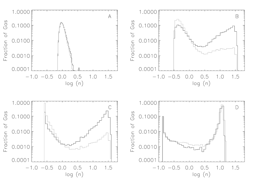
Figure 6: Panels A,B and C show the mass (black line) and volume (grey line) density PDFs for TI at the same times as the first three snapshots in Figure 4. Panel D compares the mass weighted density PDF for the standard resolution of $256^{2}$ (black line) and $512^{2}$ (grey line) at time 474 Myr.

In Figure 6, Panels A, B, and C, we plot the volume-weighted and mass-weighted density probability distribution functions (PDFs) for the first three snapshots from Figure 4. At t=14 Myr, in Panel A, all of the gas is in the unstable range. Already, though, in Panel B, after 18 Myr, the distribution has begun to separate into two distinct phases. At t=18 Myr, 69%, 28%, and 3% of the gas by volume is in the F (warm), G (unstable), and H (cold) phases respectively, which are defined by our cooling curve as the ranges $n<0.5\ {\rm cm}^{-3}$, $0.5\ {\rm cm}^{-3}<n<5.8\ {\rm cm}^{-3}$, and $5.8\ {\rm cm}^{-3}<n$, respectively. By mass these proportions are reversed to 29%, 23%, and 49%, respectively. From about 100 Myr through the end of the simulation, the distribution of cloud sizes evolves, but the PDF remains relatively unchanged, with 12%, 2%, and 86% of the mass residing in the F, G, and H phases.

We also performed the same simulation, but increased the resolution to $512^{2}$. The conduction coefficient is not changed, so $n_{c}=16$. We find similar results overall. In particular, the mass-weighted density PDFs are compared in Panel D of Figure 6. These PDFs exhibit no significant differences, confirming the robustness of our results.

3.3 Thermal Evolution

Alongside the images of density in Figure 4 we show scatter plots of $n$ against $P$ for all zones in the grid at the same times. In the initial state, pressure is constant, and $t_{sound}$ at 5 pc ($\sim 1/2$ the length of the fastest-growing TI mode) is shorter than $t_{cool}$ (see Figure 3). Towards the low density warm phase, $t_{sound}<<t_{cool}$, and gas parcels in regions undergoing rarefaction are able to heat nearly isobarically. Thus, all zones at densities lower than the mean are filled with an intercloud medium that maintains spatially nearly uniform pressure. For gas parcels undergoing compression and net cooling, as $\delta\rho$ becomes large, $t_{cool}<<t_{sound}$, so the gas tends to cool towards the thermal equilibrium curve at a faster rate than the flow is able to readjust dynamically. After gas parcels reach near thermal equilibrium in the cold phase, they continue to be compressed until pressure equilibrium with the warm medium is re-established. Over time, the average pressure in the simulation box decreases due to radiation from the cold phase.

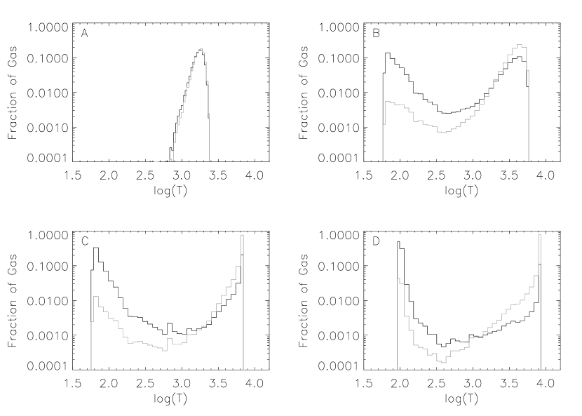
Figure 7: Mass (black line) and volume (grey line) temperature PDFs for the snapshots in Figure 4 (time increases A-D).

Because the scatter plots in Figure 4 contain a large number of points, many fall in the unstable range, although the actual amount of material there is small. To quantify this, in Figure 7 we plot mass-weighted and volume-weighted temperature PDFs at times corresponding to the snapshots in Figure 4. As with the density PDF, the distribution is separates into two distinct phases in Panel B at 18 Myr, and remains so for the duration of the simulation.

3.4 Kinetic Evolution

Thermal instability is a dynamic process, and a number of recent works have proposed that TI may help contribute to exciting turbulence in the ISM. In Figure 8 we plot the mass-weighted velocity dispersions for gas in the F, G, and H phases separately. For all phases, the largest velocities occur during the condensation stage at early times (10-20 Myr), corresponding to about 5 times the $e$-folding time of the dominant linear instability. The peak velocity is about 0.45 $\rm km\ s^{-1}$ for the unstable (G) phase, and is $\sim 0.3\ \rm km\ s^{-1}$ for the two stable phases. At later times the velocity dispersion in each phase remains relatively constant, with the largest value (0.35 $\rm km\ s^{-1}$) for phase G, next largest (0.25 $\rm km\ s^{-1}$) for the warm phase, F, and smallest (0.15 $\rm km\ s^{-1}$) for the cold phase, H. The standard deviation of the total velocity dispersion is typically 0.15 $\rm{km\ s^{-1}}$. For comparison, typical sound speeds of the F, G, and H phases are 7-8 $\rm km\ s^{-1}$ , 1-5 $\rm km\ s^{-1}$ and 0.6-1 $\rm km\ s^{-1}$, respectively. Thus, the mean turbulent velocities are all subsonic.

4 MRI Simulations

4.1 MRI Physics

In a series of four papers, Balbus & Hawley presented the first linear analysis and numerical simulations of MRI in the context of an astrophysical disk (Balbus & Hawley, 1991; Hawley & Balbus, 1991, 1992; Balbus & Hawley, 1992). The physical basis for the instability is relatively simple, and there are two requirements for the instability to be present: a differentially rotating system with decreasing angular velocity as one moves outward through the disk, and a weak magnetic field (strong magnetic fields have a stabilizing effect). As fluid elements are displaced outward (inward) the magnetic field resists shear and tries to keep the fluid moving at its original velocity. Due to these magnetic stresses, fluid elements gain (lose) angular momentum, the centrifugal force becomes too large (small) to maintain equilibrium at the new position, and the fluid element moves farther outward (inward). This leads to the transport of angular momentum outward through the disk.

For a complete linear analysis of the MRI in 2D we refer the reader to Balbus & Hawley (1991). Here we simply summarize the important formulae for axisymmetric modes with wavenumber ${\bf k}=k_{z}\hat{z}$ and ${\bf B}_{0}=B_{0}\hat{z}$. The growth rates are given by

$$\frac{\gamma^{2}}{\Omega^{2}}=\nu^{2}\left[\frac{2q-\nu^{2}}{\nu^{2}+2-q+[4\nu^{2}+(2-q)^{2}]^{1/2})}\right]$$ (8)

where $\nu\equiv k_{z}v_{{\rm A}z}/\Omega$ in terms of the Alfvén speed $v_{{\rm A}z}\equiv B_{0z}(4\pi\rho)^{-1/2}$. The maximum growth rate occurs when

$$\left(\frac{kv_{{\rm A}z}}{\Omega}\right)_{peak}=\frac{(4-(2-q)^{2})^{1/2}}{2},$$ (9)

i.e. $\lambda_{peak}=4\pi v_{{\rm A}z}/(\sqrt{3}\Omega)$ for $q=1$; here the growth rate is $\gamma_{peak}=\Omega q/2\rightarrow\Omega/2$. The highest wavenumber for which axisymmetric MRI exists when ${\bf B}_{0}=B_{0}\hat{z}$ is

$$\left(\frac{kv_{{\rm A}z}}{\Omega}\right)_{max}=\sqrt{2q}.$$ (10)

We have tested the code without cooling and conduction, and found that it can accurately reproduce the predicted linear growth rates of the MRI. We do not detail the results here; instead we refer the reader to Hawley & Balbus (1992) for a complete analysis of similar models.

Based on the linear dispersion relation, for sufficiently weak magnetic fields, modes with a range of $k_{z}$ (and also $k_{r}$) may grow. The smallest permissible wavenumber for a simulation is $(k_{z})_{min}=2\pi/L_{z}$, where $L_{z}$ is the vertical dimension of the computational box. At late times in 2D axisymmetric simulations (Hawley & Balbus, 1992), MRI becomes dominated by a “channel” solution corresponding to the smallest permissible vertical wavenumber, i.e. with flow moving towards the inner regions of the disk on one (vertical) half of the grid, and flow moving towards the outer regions in the other (vertical) half of the grid. This pure “channel flow” is unphysical; for a 3D system it is subject to nonaxisymmetric parasitic instabilities (Goodman & Xu, 1994). In 3D non-axisymmetric simulations (e.g. Hawley, Gammie, & Balbus (1995)) the channel solution forms at early times, but later develops into a fully turbulent flow.

The MRI has primarily been studied in the context of accretion disks, but can be important in any differentially rotating disk system provided the magnetic fields are not too strong. In addition to axisymmetric modes, nonaxisymmetric MRI modes can also grow directly (see e.g. Balbus & Hawley (1992) and Kim & Ostriker (2000) eqs. 80, 81 for instantaneous growth rates and instability threshold criteria in various limits). The axisymmetric mode with wavelength $\lambda_{z}\sim\rm{2H}$ is the most difficult to stabilize as $B_{z}$ increases; from equation (10), taking $\Omega=26\ \rm{km\ s^{-1}\ kpc^{-1}}$, $q=1$, a disk scale height $H$=150 pc and a uniform density $n=0.6\ {\rm cm}^{-3}$, MRI will be present provided $B_{z}<0.6\ \mu G$. For the Milky Way, this is consistent with the observed solar-neighborhood estimate $|B_{z}|=0.37\ \mu\rm G$ (Han, Manchester, & Qiao, 1999). If a multi-phase system behaves similarly to the corresponding uniform-density medium, then we may expect MRI to be important in the galactic ISM. Here, we explore how MRI development can be affected by strong non-uniformity in the density structure.

4.2 Evolutionary Development: TI + MRI Model

To study nonlinear development of the MRI in a nonuniform medium, we first perform a simulation identical to the TI model run described in § 3, but now include magnetic fields and sheared rotation. All hydrodynamical variables are initialized as described in § 3. The magnetic field is vertical with $\beta=P_{gas}/P_{mag}=1000$. The rotation rate is set to 26 km $\rm{s^{-1}\ kpc^{-1}}$ representative of the local value near the Sun, and we set the shear parameter $q=1.0$ to describe a flat rotation curve. With these parameters, from equation (10), the smallest-scale uniform-density MRI mode that would fit within our $L_{z}=100\ {\rm\,pc}$ box has $k_{z}=3$ (in units of $2\pi/L_{z}$).

On the left in Figure 9 we show snapshots of number density overlayed with magnetic field lines at three representative times, and on the right we show the corresponding mass-weighted density PDF. The time-scale for development of the MRI is much longer than that of TI, so that the initial development is essentially the same as in the purely hydrodynamical case. During the TI condensation phase the magnetic field becomes kinked as the filaments condense into small clouds. The remaining random motions of the clouds leads to further distortion of the magnetic field, as can been seen at 237 Myr. The channel solution has clearly taken hold by 474 Myr, and the $k_{z}=1$ mode (in units of $2\pi/L_{z}$) dominates.

Similarly to our analysis of kinetic evolution for the TI model, in Figure 10 we plot the velocity dispersion for the F, G, and H phases as a function of time in the TI + MRI model. Initially these are similar to the hydrodynamical case, with all velocities less than $0.5\ \rm km\ s^{-1}$. As the channel solution develops the velocity dispersion begins to increase at about 500 Myr, and peaks at the end of the simulation in phase F at approximately $1.5\ \rm km\ s^{-1}$. The peak velocity dispersion is about $1.2\ \rm km\ s^{-1}$ for phase G, and 0.9 $\rm km\ s^{-1}$ (approximately the sound speed) for phase H, all towards the end of the simulation.

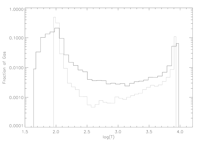
Figure 11: Mass-weighted temperature PDF for the TI run at 474 Myr (grey line) and TI + MRI at 800 Myr (black line), after the channel solution has fully developed. The active dynamics of MRI leads to the presence of high density/low temperature gas.

As in the hydrodynamical model, the PDFs for the TI + MRI model are clearly two-phase, with small amounts of gas contained in the unstable regime. At very late times the fully developed channel solution tends to increase the proportion of unstable gas. In Figure 11 we plot the mass-weighted temperature PDF of the TI + MRI model 800 Myr, and the same quantity for the TI run at 474 Myr. We do not expect that the PDF for the TI run would evolve significantly if the simulation had been continued to 800 Myr. Evidently, the dynamical flows induced by the MRI can significantly affect the temperature distribution. The larger velocity dispersion and kinked magnetic fields due to the channel solution can compress portions of cold clouds, decreasing the temperature correspondingly. Although still dominated by distinct warm and cold phases, there is also a higher proportion of gas in the unstable regime. For the same model snapshot, Figure 12 shows a $P/k$ vs. $n$ scatter plot, overlayed on the equilibrium cooling curve. In the high density regime, cooling times are short, and the gas is not far from equilibrium. At low densities cooling times are longer, and gas can be found out of thermal equilibrium.

Since the 2D channel solution would break up in a real 3D disk due to parasitic instabilities (Goodman & Xu, 1994), we do not expect the late-time effects seen in our models to have direct implications for the temperature distribution in the diffuse ISM. They illustrate, however, the more generic point that spatially-varying rotational shear coupled to magnetic fields can create stresses that force gas away from the stable equilibrium phases. We shall discuss this further, highlighting differences that might be expected for 3D MRI, in § 5.

Important questions for assessing MRI development in a cloudy medium are how the spatial- and time-scales of the fastest-growing modes differ compared to those in single-phase counterpart systems. We measure MRI mode amplitudes in the simulations by taking the Fourier transform of $B_{y}$ as a function of time, from which we can calculate the growth rates. The $k=1,2$ and 3 mode amplitudes are plotted in Figure 13. There is not an obvious linear stage from which we can measure the growth rate, but between 284 and 470 Myr the average $k=1$ growth rate is about 0.28 $\Omega$, compared to the predicted rate of 0.34 $\Omega$ at the average density of the model. At the average density linear theory predicts that the most unstable mode is at $k=2$, with a growth rate of 0.50 $\Omega$, and the $k=3$ mode is unstable as well, with a predicted growth rate of 0.41 $\Omega$. Between 284 and 470 Myr we measure a mean growth rate for the $k=2$ and $k=3$ modes to be 0.12 $\Omega$ and 0.18 $\Omega$, respectively. At the density of the warm medium, only the $k=1$ mode is predicted to be unstable in our simulations, with a growth rate of 0.45 $\Omega$. Thus, growth rates of available modes appear somewhat lower than they would be for a medium at either the mean density or the density of the warm medium. In addition, initial growth does not show the clear dominance of a single fastest growing mode that is evident in comparison adiabatic test simulations for a single-phase medium. However, at late times, the $k=1$ mode grows to exceed the other low-order modes, similarly to the findings of Hawley & Balbus (1992) for a single-phase medium.

4.3 Evolutionary Development: Cloud + MRI Model

Because the initial MRI growth in the previous model may be strongly affected by lingering dynamical effects of TI, it is of interest to consider MRI development in a medium which contains two distinct phases from the outset. In our next simulation we therefore begin with a two phase medium in approximate equilibrium, rather than developing a two phase medium from thermally unstable gas. We embed 59 high density clouds in a low density ambient medium such that the average density is the same as that of previous TI simulations. To set up the initial conditions allowing for conduction at cloud/intercloud interfaces, we first create “template” cloud profiles by embedding a single high density cold cloud in a low density warm medium and evolving until a thermally- and dynamically-relaxed state is reached. This profile (density, pressure and velocity) is then copied to randomly chosen locations on the grid, with the condition that cloud centers must be at least 20 zones apart. We initialize the magnetic field after this “cloud embedding” procedure. The simulation is then evolved as the MRI develops.

In Figure 14 we show three snapshots from the “cloud + MRI” simulation, along with mass-weighted density PDFs. The MRI takes about 500 Myr until its development begins to become apparent, as can be seen in the poloidal field lines at 464 Myr in Figure 14. At 701 Myr many of the clouds have merged and have significant velocities as the MRI channel solution begins to take hold. Initially the mass weighted density PDF shows almost no gas in the unstable range, but as the MRI begins to develop, this phase begins to become populated, and the PDF becomes very similar to those from the TI + MRI simulations.

Perhaps the most interesting results from this “cloud + MRI” simulation are the behavior of the mode amplitudes and growth rates. Initially the clouds contain negligible velocities, and are in what would be a steady state if magnetic fields were not present. We might expect, then, to find “cleaner” MRI growth rates than for the TI + MRI runs. The mode amplitudes for $k=1,2$, and 3 are plotted in Figure 15. Initially the $k=2$ mode is dominant and shows approximate linear growth between 300 Myr - 700 Myr, with an average growth rate of 0.34 $\Omega$, compared to the predicted rate 0.50 $\Omega$ at the average density. The $k=1$ mode also shows approximate linear growth with an average rate of 0.47 $\Omega$ measured from 450 Myr - 900 Myr, and becomes the dominant mode at around 800 Myr. At the density of the warm medium the theoretical growth rate of the $k=1$ mode is 0.45 $\Omega$, and at the average density it is 0.34 $\Omega$. The $k=3$ growth rate, measured between 400 Myr and 800 Myr is 0.33 $\Omega$, which we can compare to the predicted value at the average density of 0.41 $\Omega$. Thus, similarly to the TI + MRI model, growth rates are slightly lower than they would be in a medium with the same mean density. There is, however, a longer period of dominance by the mode with the fastest expected growth rate.

For comparison we also performed an MRI simulation with cooling and conduction disabled, initially at uniform density and seeded with the velocity and pressure profiles from the initial state of the previous “cloud + MRI” simulation; we also performed zero-conduction, zero-cooling test simulations seeded with random perturbations. The growth rates are in reasonable agreement between these simulations, although the case directly seeded with random perturbations had cleaner growth of mode amplitudes. Most importantly, we find that rather than $k=2$ predominating as we found in the “cloud + MRI” simulation, the $k=3$ mode in the single-phase comparison model is dominant until late time. This suggests that the initial perturbations are strongest at $k=3$, but the presence of the multi-phase medium in the “cloud + MRI” model significantly inhibits the growth of this mode because the inertial load varies strongly over a wavelength for $k=3$.

4.4 Perspective: Effects of Cloudy Structure

There are a number of ways MRI growth rates and preferred scales could be affected by the influence of a cloudy background density structure, and signs of these effects are evident in our simulations. First, both growth rates and preferred scales are dependent on the Alfvén speed, which is a function of density. The cold, dense clouds will be MRI unstable at small scales compared to the larger preferred scales of the warm, low density, ambient medium. For fixed magnetic field strength, MRI wavelengths are inversely proportional to density. Thus, MRI wavelengths in cold, dense gas will be a few parsecs, while MRI wavelengths in warm, diffuse gas will be several tens of parsecs. Although the MRI wavelengths in dense gas may be smaller than individual cold clouds, permitting initial rapid growth, further development of the small-scale instability is limited by clouds’ small radial extent. Long term MRI development must therefore have characteristic wavelengths representative of either the average density conditions or the pervasive low-density warm, intercloud gas. This expectation is indeed consistent with our results. As seen in Figures 9 and 14, both the diffuse gas and the cold clouds participate together in an overall large-scale flow. The cold clouds frequently are the sites of strong kinks in the magnetic field.

One might also expect the preferred scales for MRI to be affected by cloud spacing. If cloud spacing is small compared to a given wavelength, then the MRI growth rate might be expected to be similar to that under average density conditions. Thus, if the fastest-growing wavelength at the mean density is large compared to cloud spacing along a field line then this might be expected to be the dominant wavelength. This situation is indeed evident in the second frame (464 Myr) of Figure 14, in which the $k=2$ mode dominates, even though, as described above, the input perturbation spectrum is such that the $k=3$ mode would dominate if the density were uniform. On the other hand, if fewer, more massive clouds exist, cloud separations will be larger, which could suppress MRI growth at wavelengths shorter than cloud spacings and encourage MRI development on the largest scales. Evidence of this effect can be seen in the third panel (474 Myr) of Figure 9.

Finally, if total mass is distributed very unevenly with magnetic flux, then MRI may develop more rapidly and at longer wavelengths in regions where there is a comparatively low inertial load. In simulations (not shown) we have performed which have alternating radial zones of high and low mass loading on field lines (initiated with cold clouds at intersections in a Cartesian grid), we indeed see this effect. Development of MRI in the low-inertia “pure warm” phase is, however, checked when the radially-moving flow collides with the high-inertia cold clouds.

To test whether the growth rate of the smaller-scale k=2 mode (essentially near the lower wavelength limit for behavior as at a single average density) could be enhanced in TI+MRI models, we also performed an additional random TI simulations in which a $k=2$ perturbation was added shortly after the initial condensation phase. The perturbation was added at about the 20 percent level in $v_{1}$. For the first 500 Myr the $k=2$ mode is strongest with a growth rate of 0.36 $\Omega$. After 500 Myr the k=1 mode, with a growth rate of 0.47 $\Omega$, is again dominant.

Taken together, the simulations of this section show that the development of the MRI in the presence of a cloudy medium has modest differences compared to the corresponding development in a single phase medium at the average density. The dominant wavelengths are similar to those predicted by linear theory at mean-density conditions, and growth rates are also similar, but slightly smaller. The spacings between clouds affects which among the low-$k$ modes dominates the power during the exponential-growth phase. At very late times the $k_{z}=1$ mode is dominant in all simulations, consistent with the ultimate dominance of this channel flow in the single-phase models of Hawley & Balbus (1992).

5 Summary and Discussion

Thermal and magnetorotational instabilities may play a major role in determining the physical properties of the diffuse ISM. In regions far from active star formation or a recent supernova explosion, TI and MRI may even be the primary processes driving structure and dynamics in the ISM on scales $\lower 2.15277pt\hbox{$\;\buildrel<\over{\sim}\;$}100$ pc. The PDFs of gas density and temperature, the characteristic sizes, shapes, and spatial distributions of cloudy structures, and the amplitudes and spectral properties of turbulent velocities and magnetic fields may all be strongly influenced by TI and MRI. In addition, development and saturation of TI and MRI may be strongly interdependent. In this paper, we have initiated a study of these important processes using numerical MHD simulations. The current work focuses on code tests and 2D models using a microphysics implementation appropriate for the atomic ISM. In addition to characterizing the properties of TI and MRI modes in their nonlinear stages, this study lays the groundwork for future 3D simulations which will be used to investigate quasi-steady turbulence.

In the following, we summarize the results presented herein, compare to other recent work, and discuss key issues for future investigation.

1. Numerical methods: We have implemented atomic-ISM heating/cooling and thermal-conduction source terms in the energy equation of the ZEUS code (using implicit and explicit updates, respectively). For conditions representing the mean pressure and density in the ISM, we find excellent numerical agreement with the analytic growth rates of thermally-unstable modes for a large range of wavelengths and thermal conductivity coefficients. Based on these tests and confirmation of acceptable results for advection of high-contrast contact discontinuities (warm/cold pressure equilibrium interfaces) on the grid, we adopt a value of ${\cal K}=10^{7}\ {\rm erg}\ {\rm cm}^{-1}\ {\rm s}^{-1}\ {\rm K}^{-1}$ such that the Field length is resolved by 8 (16) zones in (100 pc)² simulations with 256² (512²) cells.

Explicit inclusion of conduction is important for suppressing numerically-unresolved TI-driven amplification of grid-scale noise; Koyama & Inutsuka (2003) have also recently highlighted the importance of implementing conduction for simulations of thermally bistable media. In some previous simulations of TI (Kritsuk & Norman, 2002a, b) under stongly cooling conditions, conduction was not included; since those simulations began with relatively large-amplitude (5%) perturbations on resolved scales, however, sub-dominant effects from unresolved growth at grid scales in the initial stages of TI would be less noticeable. In other recent work (Vázquez-Semadeni et al., 2003) simulations of TI using spectral algorithms (with explicit diffusive terms in the equations of motions) appear to have difficulty reproducing the analytic growth rates in some circumstances. Conceivably, this may be a sign of numerical diffusion that could tend to produce more gas in thermally-unstable regimes than is realistic, in simulations using these computational methods.

2. Nonlinear development of TI: In “pure TI” simulations where we initialize gas at $P/k=2000\ {\rm K}\ {\rm cm}^{-3}$ and $n=1\ {\rm cm}^{-3}$ in a (100 pc)² box with 0.1% initial pressure perturbations, we find that TI develops at a characteristic length scale consistent with the predicted fastest-growing mode, $\sim 12$ pc for our adopted value of $\cal K$. As seen in other 2D simulations (e.g. Vázquez-Semadeni, Gazol, & Scalo (2000)), the structure initially resembles a “honeycomb” network of cells, and as nonlinear development proceeds, gas condenses into cold, compact clouds at the intersections of filaments. Gas undergoing rarefaction towards the warm phase heats nearly isobarically, because the sound crossing time is short compared to the net heating-cooling time. Gas undergoing compression towards the cold phase initially has isobaric evolution (while density perturbations remain low-amplitude), but then tends first to cool toward the equilibrium curve very rapidly (with an attendant pressure drop), and then dynamically readjusts its density and temperature until the pressure again matches ambient conditions. The time to establish a distinct two-phase structure of well-separated cold clouds within a warm ambient medium (see third panel of Fig. 4) is $\sim 20$ Myr, or about 10 $e$-folding times in terms of the linear growth rate. In the subsequent evolution, the cold, dense clouds undergo successive mergers to produce larger structures.

The transition from nearly isobaric to more “isochoric”-like evolution for cold gas during nonlinear stages of condensation was recently emphasized by Burkert & Lin (2000), and snapshots of phase diagrams in Kritsuk & Norman (2002a) show a similar dip in pressure for overdense gas as it cools toward thermal equilibrium. Vázquez-Semadeni et al. (2003) found, similar to our results, that initial perturbations of similar or larger sizes to our dominant TI wavelength require times $>10$ Myr to complete the condensation process, even when a much larger (10%) initial perturbations are used. The real level of conduction in the atomic ISM may be lower than the value we adopted (for numerical efficacy), with the fastest-growing TI wavelength a factor $\sim 4$ smaller than our 12 pc value and the condensation time correspondingly shorter; Sánchez-Salcedo, Vázquez-Semadeni, & Gazol (2002) found that 3 pc-scale overdensities condense into clouds within 4 Myr. As the turbulent cascade is likely to maintain nonlinear-amplitude entropy perturbations down to sub-pc scales, we expect that the fastest-growing wavelength is likely to dominate when TI occurs under “natural” circumstances, with later mergers producing larger clouds (see also Sánchez-Salcedo, Vázquez-Semadeni, & Gazol (2002)).

3. Gas phase distributions from TI: The bimodal density and temperature PDFs in our TI simulations mirror the distinct two-phase structure evident in late-time snapshots. Typical late-time warm-, cold-, and intermediate-temperature mass fractions are 12, 86, and 2%. For a two-phase medium with mean density $\bar{n}$ and cold and warm densities $n_{\rm c}$ and $n_{\rm w}$, the fraction of mass in the cold medium is $f_{\rm c}=(1-n_{\rm w}/\bar{n})(1-n_{\rm w}/n_{\rm c})^{-1}$. Provided $n_{\rm c}\gg n_{\rm w}$, the mass fraction in the warm medium is thus $f_{\rm w}\approx n_{\rm w}/\bar{n}$. Since the pressure at late stages of our evolution has dropped near the minimum value of $P$ at which two phases are present, and in thermal equilibrium at this pressure $n_{\rm w}\approx 0.1\ {\rm cm}^{-3}$ (with $n_{\rm c}\approx 10\ {\rm cm}^{-3}$), the relative proportions of gas $f_{w}\approx 0.1,f_{c}\approx 0.9$ in the cold and warm phases are just as expected (with $\bar{n}=1\ {\rm cm}^{-3}$).

Findings on density and temperature PDFs from other recent TI simulations are varied. From the 3D simulations of Kritsuk & Norman (2002a, b), the late-time (1.5 Myr) mass fractions are $f_{\rm w}=0.42$, $f_{\rm c}=0.44$ in the stable phases and $f_{\rm i}=0.14$ in the intermediate, unstable regime. Kritsuk and Norman use a somewhat different cooling curve from ours, with $n_{\rm w}=0.4\ {\rm cm}^{-3}$ in thermal equilibrium at the minimum pressure at which two stable phases are available. Since they use $\bar{n}=1\ {\rm cm}^{-3}$, their result that $f_{\rm w}\approx n_{\rm w}/\bar{n}$ is consistent with expectations for a two-phase medium, while the gas at intermediate temperatures appears to be due to mass exchange with the cold medium (see their discussion).

In the 1D simulations of Sánchez-Salcedo, Vázquez-Semadeni, & Gazol (2002) (and using the same cooling curve and mean density as ours), only a few percent of the gas in their “multiple condensation” runs remains at intermediate densities, similar to our results, and their $f_{\rm w}=0.3-0.4$ at $t\sim 20-25$ Myr is similar to our results at comparable (early) times. In the 2D simulations of Gazol et al. (2001) that also include “stellar-like” local heat sources, the late-time mass fractions are $f_{\rm w}=0.25$, $f_{\rm c}=0.25$ $f_{\rm i}=0.50$. It is not clear to what extent this large proportion of gas at intermediate temperatures is sustained by turbulence (via adiabatic expansion/compression and/or shocks heating or cooling gas that would otherwise be in the warm or cold stable phases), versus being maintained by the localized heating turned on when $n>15{\rm cm}^{-3}$. With 3D MRI simulations in which turbulent driving is “cold”, it will be possible to address this important issue.

4. Turbulent driving by TI: We find that turbulence produced by “pure TI” has only modest amplitudes, when initiated from “average ISM” pressure and density conditions. For the warm, unstable, and cold phases, respectively, we find typical mass-weighted velocity dispersions of $0.25$, $0.35$, and $0.15$ ${\rm km\,s^{-1}}$. These velocities are all quite subsonic. In simulations starting from thermal equilibrium, Kritsuk & Norman (2002a) similarly find subsonic turbulence (${\cal M}_{rms}\sim 0.3$ at $t<$ 2Myr), although when gas is initially very hot, supersonic turbulence can be produced. When they include repeated episodes of strong UV heating Kritsuk & Norman (2002b) find Mach number variations ${\cal M}_{rms}\sim 0.2-0.6$ between “low” and “high” states; since their “low state” is dominated by cold gas with $c_{s}\sim 1\ {\rm km\,s^{-1}}$, this is consistent with our results for typical turbulent amplitudes. In the simulations of Koyama & Inutsuka (2002) in which warm gas shocks on impact with a low-density, hot ($T=3\times 10^{5}$ K) layer, TI develops near the interface of shocked gas with the hot medium, leading to the formation of cold cloudlets with velocity dispersions of a few ${\rm km\,s^{-1}}$. Although Koyama and Inutsuka attribute this turbulence to the effects of TI, it is possible that other dynamical instabilities associated with the hot/warm interface contribute in driving these motions.

5. Nonlinear development of axisymmetric MRI: We have studied the development of axisymmetric MRI under atomic ISM conditions, both with “TI+MRI” models starting from uniform density and pressure ($P/k=2000\ K\ {\rm cm}^{-3}$ and $n=1\ {\rm cm}^{-3}$), and with “cloud+MRI” models that are initiated with the same uniform pressure and total mass, but start with a population of cold clouds embedded in a warm ambient medium. The magnetic field in both types of models is vertical and initially uniform, with $B^{2}/8\pi=P/1000$. The peak growth rate of MRI (in a uniform medium) is $\Omega/2$, where $\Omega$ is the local angular velocity of the galaxy. Since this growth rate is a factor $\sim 40$ lower than typical TI growth rates, the early development of the TI+MRI model is the same as in the “pure TI” model. By the time MRI begins to develop (after a few $100$ Myr), the TI+MRI model has similar cloud/intercloud structure – except with more variations in cloud size – to the cloud+MRI model. At early times, the density and temperature PDFs are essentially the same as those produced by TI; at late times, however, while the PDFs remain bimodal, the dense gas is distributed over a somewhat larger range of densities and temperatures, due to the dynamics of the “channel flow” solution (see below).

6. Spatial scales of MRI in a cloudy medium: In both our TI+MRI and cloud+MRI simulations, after a few galactic orbital times, the velocity and magnetic fields become dominated by large-scale structures. Since the smallest-scale MRI mode that would fit in our $L_{z}=100{\rm\,pc}$ box under uniform-density conditions has vertical wavenumber $k=3$ (in units $2\pi/L_{z}$; i.e. wavelength $\lambda=L_{z}/3$), and the fastest-growing mode would have $k=2$, this implies, consistent with expectations, that cloudy density structure in the supporting medium does not grossly alter the character of MRI. We quantify MRI structural development in terms of mode amplitudes of $B_{y}$, the azimuthal magnetic field. For the TI+MRI model, the amplitudes of the $k=1,2,$ and $3$ modes are all similar – and motions in the $x-z$ plane continue to be dominated by TI effects, with cloud agglomeration – until $t\sim 400\ {\rm Myr}$, after which the clouds have become highly concentrated and the $k=1$ MRI mode associated with the “channel solution” (Hawley & Balbus, 1992) takes hold. For the cloud+MRI model, on the other hand, the $k=2$ mode grows first (with clouds remaining small and distributed) and it dominates until $\sim 800\ {\rm Myr}$, when the channel solution ($k=1$) begins to take precedence.

These differences show that the spatial distribution of clouds can have a significant effect on selecting which MRI modes are important. If intercloud distances are small compared to its wavelength, the dominant MRI mode is the same as that predicted for uniform-density conditions. If, however, other turbulent processes acting on scales small compared to MRI wavelengths (and times small compared to $\Omega^{-1}$) collect the clouds and correspondingly increase their separations, then only MRI modes at scales larger than twice the typical intercloud distance will be able to grow. As a consequence, for MRI to play an important role in the ISM, either the majority of the gas must remain in a warm, diffuse phase, or else if it collects in clouds their separations must not be too large.

It is interesting to relate these constraints to observational inferences of the HI spatial distribution. From the Heiles & Troland (2003) HI absorption observations that yielded 142 separate cold gas components on 47 lines of sight at $|b|>10^{\circ}$, their mean separation would be $\sim 40$ pc (taking the cold disk semi-thickness $\sim 100$ pc). The distribution of warm gas is much harder to interpret, but in the limiting situation where it is mainly in overdense clouds, and using Heiles and Troland’s finding that $\sim 25\%$ of emission components have no associated absorption, the mean distance between clouds would be $\sim 30$ pc. Intercloud separations similar to these estimates are small enough that vertical MRI modes could be supported; if cloud spacings are appreciably larger, however, they could not be.

7. Growth rates and saturation amplitudes of MRI: For the low-$k$ modes that are present in both our TI+MRI and cloud+MRI models, typical growth rates are generally comparable to those for modes of the same wavelength in a medium of the same mean density. For the TI+MRI model, typical growth rates are measured to be $0.28\ \Omega$, $0.12\ \Omega$, and $0.18\ \Omega$ for the $k=1$, 2, and 3 modes, respectively, compared to the rates $\gamma/\Omega=0.45$, $0.5$, and $0.41$ that would apply for a uniform medium. For the cloud+MRI model, the exponential MRI growth is “cleaner”; rates are $\gamma/\Omega=0.47$, $0.34$, and $0.33$ for $k=1$, 2, and 3 modes, respectively. The growth rates of smaller-scale ($k=2,3$) modes are thus slightly more affected by the presence of cloudy structure than that of the largest-scale ($k=1$) mode, consistent with expectations.

Although definitive results await 3D simulations, these findings provide support for the possibility that MRI may drive turbulence in the diffuse ISM at amplitudes consistent with observations of HI emission and absorption. From previous 3D simulations under relatively uniform conditions (accomplished by adopting an isothermal equation of state), the velocity dispersions driven by MRI in steady-state were found to be smaller than observed values. In particular, Kim, Ostriker, & Stone (2003) found that the typical 1D turbulent amplitudes are 3 - 4 ${\rm km\,s^{-1}}$, whereas the observed nonthermal contribution to the 1D velocity dispersion for both cold and warm gas amounts to $\sigma_{v}\sim 7\ {\rm km\,s^{-1}}$ (Heiles & Troland, 2003). Thus, for a single phase medium, MRI-driven turbulent velocity amplitudes in steady state – which are determined by a balance between excitation and dissipation – fall a factor $\sim 2$ short of explaining observations.

Since our present cloudy-medium models show growth rates quite comparable to those in a one-phase medium, the key question is therefore whether MRI dissipation rates are reduced in a cloudy medium, and if so, whether the reduction can yield a factor two increase in $\sigma_{v}$. To see that a quantitative effect at this level is not unreasonable, consider the comparison to an idealized system of ${\cal N}_{cl}\equiv\ell^{-3}$ clouds per unit volume having individual radii $r$, internal density relative to the mean value $n_{cl}/\bar{n}$, and RMS relative velocity dispersion $\sigma_{v}$. With turbulent energy driving and dissipation rates $\dot{\cal E}_{in}$ and $\sim\sigma_{v}^{2}/t_{coll}$, where the collision time $t_{coll}=(4\sqrt{\pi}r^{2}{\cal N}_{cl}\sigma_{v})^{-1}$, $\sigma_{v}$ in steady state is an order-unity factor times $(\dot{\cal E}_{in}\ell)^{1/3}(n_{cl}/\bar{n})^{2/9}$. For this idealized situation, concentrating material into clouds with $n_{cl}/\bar{n}\sim 30$ (similar to cold ISM clouds) would indeed increase $\sigma_{v}$ by a factor two compared to the case with near-uniform conditions, $n_{cl}/\bar{n}\sim 1$. With 3D simulations, it will be possible to test whether a similar scaling behavior holds for the saturated state of MRI-driven turbulence in cloudy vs. single-phase ISM models.

Figure 1: Theoretical thermal instability growth rates (Field, 1965) for varying levels of conduction $\mathcal{K}=7.48\times 10^{6},10^{7},10^{8}$ (curves as indicated), overlayed with measured growth rates (points) from test simulations. For reference we include the theoretical curves for $\mathcal{K}=0$ and for our chosen value of $\mathcal{K}=1.03\times 10^{7}\ \rm{erg\ cm^{-1}\ K^{-1}\ s^{-1}}$, as well as using an estimate of the physical conduction in the ISM at 2000K, $\mathcal{K}=1.12\times 10^{5}\ \rm{erg\ cm^{-1}\ K^{-1}\ s^{-1}}$. The asymptotic growth rate at small scales is $(2\ \rm{Myr})^{-1}$ for the adopted parameters.

Figure 2: Advection test results (crosses) compared with the initial profile (solid line) of a 1D cloud. In Panel A we show results from the original ZEUS-2D code, without cooling and conduction. In Panels B, C, and D we set the conduction parameter so that $n_{c}=$ 8, 16, and 32, respectively. Advection test results improve as $n_{c}$ increases.

Figure 3: Comparison of $t_{cool,eff}$ and $t_{sound}$ as a function of density for $P/k=2000$ and $\ell=5\ {\rm\,pc}$. For range of $0.1\ \rm{cm^{-3}}\lesssim n\lesssim 1\ \rm{cm^{-3}}$ the sound crossing time is less than the effective cooling time, so that gas can evolve at approximately constant pressure. For higher densities, $t_{cool,eff}$ is typically an order of magnitude shorter than $t_{sound}$, and the gas tends to cool towards the equilibrium curve. The peaks where $t_{cool,eff}$ approaches infinity represent the equilibrium densities (n= 0.29 $\rm{cm^{-3}}$, 0.78 $\rm{cm^{-3}}$, 32 $\rm{cm^{-3}}$) at which heating and cooling rates are equal for $P/k=2000$.

Figure 4: Density evolution in the TI simulation. Left: snapshots of $\log(n)$ at representative times as noted. Right: scatter plots of $n$ and $P/k$ from the simulation, together with the equilibrium cooling curve and the labeled temperature contours that demark the transitions between the F, G, and H phases.

Figure 5: Power spectrum of the TI density distribution at 14 Myr.

Figure 8: Evolution of velocity dispersion = $(v_{x}^{2}+v_{z}^{2})^{1/2}$ in the TI model. Typical velocities for the F (warm), G (unstable), and H (cold) phases are $0.35\ {\rm km}\ {\rm s}^{-1}$, $0.25\ {\rm km}\ {\rm s}^{-1}$, and $0.15\ {\rm km}\ {\rm s}^{-1}$.

Figure 9: Structural evolution of the TI + MRI simulation. Left: snapshots of $\log(n)$ at representative times as noted, overlayed with magnetic field lines. Right: mass-weighted density PDF at the same times as the snapshots.

Figure 10: Mass-weighted velocity dispersion = $(v_{x}^{2}+v_{z}^{2})^{1/2}$ for TI + MRI model, separated by phase. The initial velocity dispersion is due to the development of TI (see Figure 8). After 400 Myr the MRI becomes important, and the channel solution increases the velocity dispersion to as high as 1.4 ${\rm km}\ {\rm s}^{-1}$ towards the end of the simulation.

Figure 12: Scatter plot of $n$ and $P/k$ at 800 Myr, near the end of the simulation, for the TI + MRI model. Cooling timescales are short for the high density gas, so gas remains near thermal equilibrium for a range of pressures. In the low density regime, cooling time-scales are longer, and there can be significant departures from thermal equilibrium.

Figure 13: Mode amplitudes for $B_{y}$ in the TI + MRI model. For the first 500 Myr the $k=1,2$ and 3 modes are approximately equal in amplitude, but the $k=1$ mode is dominant after this point.

Figure 14: Structural evolution of cloud + MRI simulation. Left: snapshots of $\log(n)$ at representative times as noted, overlayed with magnetic field lines. Right: mass-weighted density PDF at the same times as the snapshots.

Figure 15: Mode amplitudes of $B_{y}$ in the cloud + MRI simulation. The $k=2$ mode is initially the largest, but by the end of the simulation the $k=1$ mode has become dominant.

References

- Balbus & Hawley (1991) Balbus, S. A. & Hawley, J.F. 1991, ApJ, 376, 214
- Balbus & Hawley (1992) Balbus, S. A. & Hawley, J.F. 1992, ApJ, 400, 610
- Burkert & Lin (2000) Burkert, A. & Lin, D.N.C 2000, ApJ, 537, 270
- de Avillez (2000) de Avillez, M.A. 2000, MNRAS, 315, 479
- Cox & Smith (1974) Cox, D.P. & Smith, B.W. 1974, ApJ, 189, L105
- Dickey & Lockman (1990) Dickey, J.M. & Lockman, F.J. 1990 ARA&A, 28, 215
- Evans & Hawley (1988) Hawley, J. F. & Evans, C.R. 1988 ApJ, 332, 659
- Field (1965) Field, G.B. 1965 ApJ, 142, 531
- Field, Goldsmith, & Habing (1969) Field, G.B., Goldsmith, D.W., & Habing, H.J. 1969, ApJ, 155, 149
- Ferrara & Shchekinov (1993) Ferrara, A. & Shchekinov, Y. 1993, ApJ, 417, 595
- Fitzpatrick & Spitzer (1997) Fitzpatrick, E.L., & Spitzer, L., Jr. 1997, ApJ, 475, 623
- Gazol et al. (2001) Gazol, A., Vázquez-Semadeni, E., Sánchez-Salcedo, F.J., & Scalo, J. 2001, ApJ, 557, L121
- Goodman & Xu (1994) Goodman, J. & Xu, G. 1994 ApJ, 432, 213
- Han, Manchester, & Qiao (1999) Han, J.L., Manchester, R.N., & Qiao, G.J. 1999, MNRAS, 306, 371
- Hawley & Balbus (1991) Hawley, J. F. & Balbus, S. A. 1991, ApJ, 376, 223
- Hawley & Balbus (1992) Hawley, J. F. & Balbus, S. A. 1992, ApJ, 400, 595
- Hawley, Gammie, & Balbus (1995) Hawley, J. F., Gammie, C.F., & Balbus, S. A., ApJ, 440, 742
- Hawley & Stone (1995) Hawley, J. F., & Stone, J.M. 1995 Computer Physics Communications, 89, 127
- Heiles (2001) Heiles, C. 2001, ApJ, 551, L105
- Heiles & Troland (2003) Heiles, C. & Troland, T.H. 2003, ApJ, 586, 1067
- Hennebelle & Pérault (1999) Hennebelle, P. & Pérault, M. 1999, A&A, 351, 309
- Jenkins (2003) Jenkins, E.B. 2003, astroph-0303266
- Kalbera, Schwarz, & Goss (1985) Kalberla, P. M. W., Schwarz, U. J., & Goss, W. M. 1985, A&A, 144, 27
- Kim & Ostriker (2000) Kim, W. & Ostriker, E.C. 2000, ApJ, 540, 372
- Kim & Ostriker (2001) Kim, W. & Ostriker, E.C. 2001, ApJ, 559, 70
- Kim, Ostriker, & Stone (2003) Kim, W., Ostriker, E.C., & Stone, J.M. 2003, ApJ, submitted
- Korpi et al. (1999) Korpi, M.J., Brandenburg, A., Shukurov, A., Tuominen, I., & Nordlund, Å. 1999, ApJ, 514, L99
- Koyama & Inutsuka (2002) Koyama, H. & Inutsuka, S. 2002, 564, L97
- Koyama & Inutsuka (2003) Koyama, H. & Inutsuka, S. 2003, astroph-0302126
- Kritsuk & Norman (2002a) Kritsuk, A.G. & Norman, M.L. 2002a, ApJ, 569, L127
- Kritsuk & Norman (2002b) Kritsuk, A.G. & Norman, M.L. 2002b, ApJ, 580, L51
- Mac Low et al. (2001) Mac Low, M., Balsara, D., Avillez, M.A., & Kim, J. 2001, astroph
- McKee & Ostriker (1977) McKee, C.F. & Ostriker, J.P. 1977, ApJ, 218, 148
- Parker (1953) Parker, E.M. 1953, ApJ, 117, 431
- Press et al. (1992) Press, W.H., Teukolsky, S.A., Vetterling, W.T., & Flannery, B.P. 1992, Numerical Recipes in C, Second Edition (Cambridge:Cambridge University Press)
- Rosen & Bregman (1995) Rosen, A. & Bregman, J.N. 1995, ApJ, 440, 634
- Sánchez-Salcedo, Vázquez-Semadeni, & Gazol (2002) Sánchez-Salcedo, F.J., Vázquez-Semadeni, E., & Gazol, A. 2002, ApJ, 577, 768
- Sellwood & Balbus (1999) Sellwood, J.A. & Balbus, S.A. 1999, ApJ, 511, 660
- Spitzer (1978) Spitzer, L., Jr. 1978, Physical Processes in the Interstellar Medium (New York:Wiley)
- Spitzer & Fitzpatrick (1995) Spitzer, L., Jr.& Fitzpatrick, E.L. 1995, ApJ, 445, 196
- Stone et al. (1996) Stone, J. M., Hawley, J.F, Gammie, C.F, & Balbus, S.A. 1996, ApJ, 463, 656
- Stone & Norman (1992a) Stone, J. M. & Norman, M. L. 1992a, ApJ, 80, 753
- Stone & Norman (1992b) Stone, J. M. & Norman, M. L. 1992b, ApJ, 80, 791
- Truelove et al. (1997) Truelove, J.K., Klein, R.I., McKee, C.F., Holliman, J.H., II, Howell, L.H., & Greenough, J.A. 1997, ApJ, 489, L179
- Vázquez-Semadeni, Gazol, & Scalo (2000) Vázquez-Semadeni, E., Gazol, A., & Scalo, J. 2000, ApJ, 540, 271
- Vázquez-Semadeni et al. (2002) Vázquez-Semadeni, E., Gazol, A., Passot, T., & Sánchez-Salcedo, J. 2002, astroph
- Vázquez-Semadeni et al. (2003) Vázquez-Semadeni, E., Gazol, A., Passot, T., Sánchez-Salcedo, J. 2003, in Turbulence and Magnetic Fields in Astrophysics, eds. E. Falgarone and T. Passot, (Berlin:Springer-Verlag) p. 213
- Verschur & Magnani (1994) Verschuur, G.L., & Magnani, L. 1994, AJ, 107, 287
- Wada & Norman (1999) Wada, K. & Norman, C.A. 1999, ApJ, 516, L13
- Wada, Spaans, & Kim (2000) Wada, K., Spaans, M., & Kim, S. 2000, ApJ, 540, 797
- Wada & Norman (2001) Wada, K. & Norman, C.A. 2001a, ApJ, 547, 172
- Wada (2001) Wada, K. 2001b, ApJ, 559, L41
- Wada & Koda (2001) Wada, K. & Koda, J. 2001c, PASJ, 53, 1163
- Wada, Meurer, & Norman (2002) Wada, K., Meurer, G., & Norman, C.A. 2002, ApJ, 577, 197
- Wolfire et al. (1995) Wolfire, M.G., Hollenbach, D., Mckee, C.F., Tielens, A.G.G.M., & Bakes, E.L.O. 1995, ApJ, 443, 152
- Wolfire et al. (2003) Wolfire, M.G, Mckee, C.F., Hollenbach, D., & Tielens, A.G.G.M. 2003, ApJ, 587, 278