Uncertainties in stellar abundance analyses

Abstract

Over the last half-century quantitative stellar spectroscopy has made great progress. However, most stellar abundance analyses today still employ rather simplified models, which can introduce severe systematic errors swamping the observational errors. Some of these uncertainties for late-type stars are briefly reviewed here: atomic and molecular data, stellar parameters, model atmospheres and spectral line formation.

Research School of Astronomy and Astrophysics, Mt Stromlo Observatory, Cotter Rd, ACT 2611, Australia (martin@mso.anu.edu.au)

1. Introduction

In view of the central role stellar abundance analyses play in the endeavours to decipher the formation and evolution of stars, galaxies and indeed the Universe as a whole, minimizing systematic errors should be of utmost importance. Certainly, there are many potential fallacies that can be made in the process of going from an observed stellar spectrum to the extracted chemical composition of the star, all which deserves very careful consideration. Unfortunately, this is an area which often has not received the attention its importance warrants. Instead, still today most elemental abundance analyses of late-type stars rely on very simplified models for the stellar atmospheres and the spectral line formation processes. Unfortunately, the progress in modelling has not kept up with the dramatic improvements on the observational side over the last couple of decades, leaving the error budget normally dominated by systematic uncertainties.

Due to page restrictions this review focus only on the uncertainties in the derived elemental abundances introduced during the numerical analyses. Potential observational pitfalls such as signal-to-noise, resolving power, fringing, scattered light, continuum placement and blends can certainly also be major sources of error, but are not discussed here. Furthermore, the review is limited to late-type stars as they have traditionally been the most widely used beacons when tracing Galactic chemical evolution. The reader is referred to Werner et al. (2002) for an account of current hot star modelling, which is becoming increasingly important when probing environments beyond our own Galaxy.

2. Atomic and molecular data

The most obvious input data needed to derive elemental abundances is the transition probability, normally expressed as the $gf$-value. While there is always a continuing need for more and better data in this respect, the overall situation is in fact relatively good today. Provided the stellar spectroscopists are prepared to search the physics literature and databases, there are many accurate experimental and computational $gf$-determinations available (e.g. http://physics.nist.gov). The Kurucz database (http://kurucz.harvard.edu) is a very valuable resource but the drawback with such a large-scale computational effort is that individual transitions can be very erroneous, in particular when involving predicted energy levels. Other necessary data (continuous opacities, line broadening, dissociation energies etc) are also in general in reasonably healthy shape now (e.g. Seaton et al. 1994; Barklem et al. 2000), although improvements are certainly encouraged.

As will be discussed further below, the formation of a spectral line depends in principle not only on the line itself but on all other lines also, including those of other elements. In order to compute the statistical equilibrium of a species one needs not only transition probabilities for all relevant lines but also photo-ionization and collisional cross-sections. In terms of photo-ionization there has been marked improvements recently with the advent of large opacity calculations like Opacity Project and Iron Project (e.g. Seaton et al. 1994). For elements up to the Fe-peak the situation is now fairly healthy for late-type stars. The most pressing uncertainty in non-LTE studies today is the cross-sections for collisional excitation and ionization with electrons and hydrogen atoms. The Opacity Project has partly addressed the case of electron collisions but most calculations largely rely on classical recipes like van Regemorter’s (1963) formula. The situation for inelastic H collisions is even worse with the approach of Drawin (1968) mostly used. The few existing experimental and quantum mechanical calculations suggests, however, that the Drawin recipe over-estimates the cross-sections by about three orders of magnitude, at least for Na and Li (e.g. Fleck et al. 1991; Barklem et al. 2003). Whether this is true for all elements is not known. Clearly there is a great need for more quantum mechanical calculations addressing this fundamental problem.

3. Stellar parameters

We will here limit the discussion to methods more universally used, noting that in special situations other more accurate options are available (interferometry, eclipsing binaries etc).

Of the fundamental stellar parameters, $T_{\rm eff}$ is normally the most crucial in order to obtain accurate abundances. There exists a multitude of methods to determine $T_{\rm eff}$ of varying model dependence and reliability. Of these, the infrared flux method (IRFM, Blackwell & Shallis 1977) is often advocated as the best. IRFM is based on the ratio of bolometric flux ($\propto T_{\rm eff}^{4}$ and reddening- and model-independent) with an IR monochromatic flux ($\propto T_{\rm eff}$ and essentially reddening- and model-independent). If the problem of collecting sufficiently accurate (spectro-)photometry can be overcome, IRFM should yield temperatures to better than 50 K (Alonso et al. 1996). Photometric $T_{\rm eff}$ determinations can be almost as good when using colours like $V-K$ and $b-y$ (corrected for interstellar reddening if significant), in particular if calibrated to an IRFM- or interferometric temperature scale (Bessell et al. 1998). As always with theoretical colours, the zero-point is an outstanding issue.

In principle, hydrogen Balmer lines should be sensitive thermometers but practical problems unfortunately limit their usefulness, not the least observational. The Balmer lines are formed in deep atmospheric layers where convective energy transport is important for setting the temperature structure. The classical mixing length theory for convection in 1D models is unlikely to capture all aspects in this transition from convection to radiation, as will be further discussed below. The line broadening, including self-broadening, of the H lines have recently been improved (Barklem et al. 2002) but these results have not yet been fully disseminated into the wider astronomical community, leading to unnecessary additional errors. At solar metallicities H lines could in the best cases yield $T_{\rm eff}$ to within about 100 K but the uncertainties become progressively worse for metal-poor stars. The use of for example excitation balance of Fe i and other lines and various line-depth ratios can achieve highly precise relative temperatures for similar stars but due to possible non-LTE and 3D effects can not be expected to give accurate absolute values. In summary, $T_{\rm eff}$ can under favourable circumstances be determined to within 100 K, which corresponds to abundance errors of typically 0.1 dex.

The surface gravities are often the most poorly constrained parameter. With the advent of the Hipparcos astrometry the situation has improved dramatically, at least for the stars sufficiently nearby to show measurable parallaxes. Knowing the parallax, the observed magnitude can be converted to a surface gravity: ${\rm log}g/g_{\hbox{$\odot$}}={\rm log}{\cal M}/{\cal M}_{\hbox{$\odot$}}+4\cdot{\rm log}\mbox{$T_{\rm eff}$}/T_{{\rm eff,}\hbox{$\odot$}}+0.4\cdot(M_{\rm bol}-M_{{\rm bol,}\hbox{$\odot$}}).$ The uncertainty is normally dominated by the parallax error going into $M_{\rm bol}$ but if $\Delta\pi/\pi<0.2$, log $g$ can be determined to within 0.2 dex (e.g. Nissen et al. 1997). The Strömgren $c_{1}$-index and isochrone-fitting can also be employed to estimate log $g$ but are more uncertain. The pressure-sensitive wings of strong lines, such as the Mg ib triplet (Blackwell & Willis 1977) is a good gravity-meter with the caveat of potential systematic errors due to non-LTE and 3D effects, which have not yet been fully assessed. One of the most commonly used techniques is to force ionization balance between neutral and ionized species such as Fe i/Fe ii and Ti i/Ti ii. In the absence of any of the above-mentioned procedures, this is a viable option but it must be realised that the result may be very severe errors in log $g$. Due to over-ionization of neutral minority species (e.g. Fe i) compared with the LTE predictions, this method typically underestimates the gravity by up to 0.5 dex or even more (Thevenin & Idiart 1999). For pressure-sensitive spectral features like molecular lines this can obviously be disastrous. A good habit is to ratio two equally gravity-sensitive species like C i, O i, S i and Fe ii to obtain abundance ratios (e.g. Nissen et al. 2002, 2003; Akerman et al. 2003).

In view of the potentially large non-LTE effects and 3D effects on Fe i lines discussed below, the preferred choice for the metallicity determinations is no doubt Fe ii lines, which are largely immune to such problems (e.g. Thevenin & Idiart 1999; Asplund et al. 1999). This should yield [Fe/H] values accurate to typically within 0.1-0.2 dex, depending on how well $T_{\rm eff}$ and log $g$ can be constrained. The alternative method on relying on colours, in particular Strömgren photometry, normally gives reasonable results with uncertainties $\mathrel{\hbox{\hbox to0.0pt{\hbox{\lower 4.0pt\hbox{$\sim$}}\hss}\hbox{$<$}}}0.3$ dex when properly calibrated. Any error in [Fe/H] naturally directly propagates into the derived [X/Fe] ratios, re-enforcing the need for a simultaneous [Fe/H] determination together with the other elements rather than relying on literature values.

4. Stellar model atmospheres

The vast majority of abundance analyses of late-type stars rely on model atmospheres which are 1D, time-independent and hydrostatic, which assume LTE and treat convection with the rudimentary mixing length theory. Even a casual glance at the solar surface reveals that these assumptions and approximations are very disputable. The question is whether this propagates into significant systematic errors in the derived abundances? Recently realistic 3D time-dependent hydrodynamical simulations of stellar surface convection and atmosphere with a detailed treatment of radiative transfer and state-of-the-art equation-of-state and opacities have become available for solar-type stars (e.g. Nordlund & Dravins 1990; Stein & Nordlund 1998; Asplund et al. 1999; Asplund & García Pérez 2001). They successfully reproduce a wide range of observational diagnostics (granulation topology, helioseismology, intensity brightness contrasts, spectral line shapes, shifts and asymmetries etc). It therefore appears that one can place a fairly high degree of confidence in their ability in describing the real stellar atmospheres, in spite of the simplifications necessary in order to carry out the simulations, most notably in terms of numerical resolution and radiative transfer. A notable achievement is that the traditional free parameters of stellar spectroscopy (mixing length parameters, micro- and macroturbulence) have become obsolete with 3D models, greatly reducing the uncertainties.

This new generation of 3D hydrodynamical model atmospheres have started to be applied to stellar abundance analyses. For the Sun, this has caused a very substantial reduction (0.2-0.3 dex) in the solar C, N and O abundances (Allende Prieto et al. 2001, 2002; Asplund et al. 2003b). For the first time, all different diagnostics (permitted, forbidden and molecular lines) give concordant abundances. The new results are also supported by the excellent agreement between observed and predicted line shapes and center-to-limb variations. Other, less temperature-sensitive elements like Si and Fe only show small ($\mathrel{\hbox{\hbox to0.0pt{\hbox{\lower 4.0pt\hbox{$\sim$}}\hss}\hbox{$<$}}}0.05$ dex) 3D abundance corrections (Asplund et al. 2000). The exact 3D effects depend on the ionization stage, excitation potential and strength of the line in question.

The most dramatic differences with standard 1D analyses appears at low metallicities. Due to much lower temperatures in the optically thin layers in the metal-poor 3D models as a result of the shift in balance between expansion cooling and radiative heating, many spectral features are greatly affected (Asplund et al. 1999). In particular molecular lines but also low excitation lines and neutral minority species tend to have large negative 3D abundance corrections in metal-poor stars (i.e. 1D analyses over-estimate the abundances). As a result, Fe i lines are very unreliable but Fe ii lines, which are formed in deeper atmospheric layers where the differences between 3D and 1D models are much smaller, are quite robust. In some cases additional 3D non-LTE effects can conspire to give final results quite close to the 1D non-LTE case, as for Li (Asplund et al. 2003a), but this is obviously not generally true. In the absence of detailed 3D non-LTE calculations, we advise against using Fe i and such species. Extreme caution must be exercised when relying on resonance and other low excitation lines (Al, Mg, Sr, Ba, Eu etc) in halo stars, where the systematic errors may well be $-0.3$..$-0.5$ dex. The largest errors, however, occur for molecular lines (Fig. 1) for which the 1D analyses can overestimate the abundances by up to 1.0 dex at [Fe/H] $=-3$ (Asplund & García Pérez 2001; Asplund 2003). Needless to say, such large systematic errors can have a profound impact on the interpretations in terms of stellar nucleosynthesis and galactic chemical evolution.

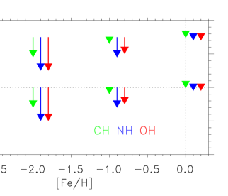
Figure 1.: The typical 3D abundance corrections relative to the Sun for CH, NH and OH (A-X) lines reveal a strong metallicity dependence.

5. Spectral line formation

Spectral line formation essentially always occurs as a non-equilibrium process: under typical atmospheric conditions radiative rates dominate over collisional rates and the radiation field departs from the Planck function. Non-LTE line formation is therefore neither special nor unusual, while LTE line formation is: LTE is an extreme assumption, not a cautious middle-ground. Of course, in many incidences the different line formation processes are such that LTE-based abundances are indeed good approximations but that must always be confirmed a posteriori by detailed non-LTE calculations (e.g. Fe ii). In general, non-LTE effects become progressively worse for higher $T_{\rm eff}$ (higher $J_{\nu}$) and lower log $g$ (less collisions) and [Fe/H] (less e^- collisions and stronger UV radiation field).

In spite of the availability of efficient and user-friendly non-LTE codes such as multi (Carlsson 1986), not enough work has been devoted to this important area. Amazingly, detailed non-LTE studies of solar-type and metal-poor stars have been undertaken for only a dozen elements or so. Typical non-LTE abundance corrections for halo stars are $0.2-0.3$ dex of either sign (e.g. Be ii, O i, Mg i, K i, Ca i, Fe i, Sr ii, Ba ii) but significantly larger in cases like Al i and B i (Kiselman 1994). It is true that the poorly known H collision cross-sections introduce uncertainties (e.g. Korn et al. 2003) but calculations with and without the classical Drawin (1968) recipe should bracket the expected non-LTE effects; as already mentioned, the available evidence suggests that the Drawin formula over-estimates the H collisions by about three orders of magnitude.

The lack of non-LTE calculations for the majority of elements severely hampers our understanding of stellar nucleosynthesis and galactic chemical evolution. For example, it is not known whether the recently discovered upturn in [C/O] at the lowest [Fe/H] is due to C production in Pop III stars or can be explained by differential non-LTE effects between C i and O i (Akerman et al. 2003). Clearly, there is huge need for more non-LTE investigations for more elements.

Acknowledgments.

I thank the organizers (Poul Erik Nissen and Max Pettini) and the other JD15 participants for creating a stimulating meeting. This talk is available at http://www.mso.anu.edu.au/$\sim$martin/talks/Sydney03_jd15).

References

Akerman, C.J., Carigi, L., Nissen, P.E., et al. 2003, A&A, in press

Allende Prieto, C., Lambert, D.L., & Asplund, M. 2001, ApJ, 556, L65

Alonso, A., Arribas, S., & Martinez-Roger, C. 1996, A&AS, 117, 227

Asplund, M., 2003, ApJL, submitted

Asplund, M., Carlsson, M., & Botnen, A.V. 2003a, A&A, 399, L31

Asplund, M., & García Pérez, A.E. 2001, A&A, 372, 601

Asplund, M., Grevesse, N., Sauval, A.J., et al. 2003b, A&A, submitted

Asplund, M., Nordlund, Å., Trampedach, R., & Stein, R.F. 1999, A&A, 346, L17

Asplund, M., Nordlund, Å., Trampedach, R., & Stein, R.F. 2000, A&A, 359, 743

Barklem, P.S., Belyaev, B.K., & Asplund, M. 2003, A&A, in press

Barklem, P.S., Piskunov, N., & O’Mara, B.J. 2000, A&AS, 142, 467

Barklem, P.S., Stempels, H.C., Allende Prieto, C. et al. 2002, A&A, 385, 951

Bessell, M.S., Castelli, F., & Plez, B. 1998, A&A, 333, 231

Blackwell, D.E., & Shallis, M.J. 1977, MNRAS, 180, 177

Blackwell, D.E., & Willis, R.B. 1977, MNRAS, 180, 169

Carlsson, M. 1986, Uppsala Astronomical Report No. 33

Drawin, H.W. 1968, Z. Physik, 211, 404

Fleck, I., Grosser, J., Schnecke, A., et al. 1991, JPhysB, 24, 4017

Kiselman, D. 1994, A&A, 286, 169

Korn, A.J., Shi, J., & Gehren, T. 2003, A&A, 407, 691

Nissen, P.E., Chen, Y.Q., Asplund, M., & Pettini, M. 2003, A&A, submitted

Nissen, P.E., Høg, E., & Schuster, W.J. 1997, in: ESA $Hipparcos$ Symp., 225

Nissen, P.E., Primas, F., Asplund, M., & Lambert, D.L. 2002, A&A, 390, 235

Nordlund, Å., & Dravins, D. 1990, A&A, 228, 155

Seaton, M.J., Yan, Y., Mihalas, D., & Pradhan, A.K., 1994, MNRAS, 266, 805

Stein, R.F., & Nordlund, Å. 1998, ApJ, 499, 914

Thévenin, F., & Idiart, T. 1999, ApJ, 521, 753

van Regemorter, H. 1962, ApJ, 136, 906

Werner, K., et al. 2002, in: Stellar atmosphere modelling [astro-ph/0209535]