Globular cluster abundances in the light of 3D hydrodynamical model atmospheres

Abstract

The new generation of 3D hydrodynamical model atmospheres have been employed to study the impact of a realistic treatment of stellar convection on element abundance determinations of globular cluster stars for a range of atomic and molecular lines. Due to the vastly different temperature structures in the optically thin atmospheric layers in 3D metal-poor models compared with corresponding hydrostatic 1D models, some species can be suspected to be hampered by large systematic errors in existing analyses. In particular, 1D analyses based on minority species and low excitation lines may overestimate the abundances by $>0.3$ dex. Even more misleading may be the use of molecular lines for metal-poor globular clusters. However, the prominent observed abundance (anti-)correlations and cluster variations are largely immune to the choice of model atmospheres.

1 Introduction

Determining stellar element abundances play a crucial role in the efforts to improve our understanding of formation and evolution of globular clusters. The term observed abundances is somewhat of a misnomer however, since the chemical composition can not be inferred directly from an observed spectrum. The obtained stellar abundances are therefore never more trustworthy than the models of the stellar atmospheres and the line formation processes employed to analyse the observations. Traditionally, abundance analyses of late-type stars rely on a number of assumptions, several of which are known to be of quite questionable nature. In standard analyses, the employed model atmospheres are one-dimensional (1D, either plane-parallel or spherical), time-independent, static and assumed to fulfull hydrostatic equilibrium. Energy transport by convection is approximated by the rudimentary mixing-length theory while otherwise radiative equilibrium is enforced. Furthermore, local thermodynamic equilibrium (LTE) is normally assumed both for the construction of the model atmospheres and in the spectrum synthesis. It should come as no surprise that abundance analyses performed along these lines may well contain significant systematic errors due to the adopted simplifications and approximations.

Perhaps the most severe shortcoming in standard analyses is the treatment of convection. For late-type stars, the surface convection zone reaches the stellar atmosphere, which thereby directly affects the emergent spectrum. The solar granulation is the observational manifestation of convection: concentrated, rapid, cold downdrafts in the midst of broad, slow, warm upflows. Qualitatively similar granulation properties are expected in other solar-type stars, as indeed confirmed by 3D numerical simulations (e.g. Nordlund & Dravins 1990; Asplund et al. 1999; Asplund & García Pérez 2001; Allende Prieto et al. 2002) and indicated by observed spectral line asymmetries. The up- and downflows have radically different temperature structures (Stein & Nordlund 1998), which can not be approximated by normal theoretical 1D hydrostatic model atmospheres with different effective temperatures $T_{\rm eff}$ (Fig. 1). Because of the photospheric inhomogeneities and the highly non-linear and non-local nature of spectrum formation, it is clear that no single 1D model can be expected to properly describe all aspects of what is inherently a 3D phenomenon (e.g. Asplund et al. 2003b).

Here I will describe recent progress in developing 3D hydrodynamical model atmospheres of late-type stars and their applications to stellar abundance analyses, in particular for elements relevant for globular cluster studies.

2 3D hydrodynamical model atmospheres

The 3D model atmospheres which form the basis of the abundance analyses presented here have been computed with a 3D, time-dependent, compressible, explicit, radiative-hydrodynamics code developed to study solar and stellar surface convection (Stein & Nordlund 1998). The hydrodynamical equations for conservation of mass, momentum and energy are solved on a Eulerian mesh with gridsizes of $\approx 100^{3}$ with explicit time-integration. The physical dimensions of the grids are sufficiently large to cover many ($>10$) granules simultaneously in the horizontal direction and about 13 pressure scale-heights in the vertical. In terms of continuum optical depth the simulations extend at least up to log $\tau_{\rm Ross}\approx-5$ which for most purposes are sufficient to avoid numerical artifacts of the open upper boundary on spectral line formation. The lower boundary is located at large depths to ensure that the inflowing gas is isentropic and featureless, while periodic horizontal boundary conditions are employed.

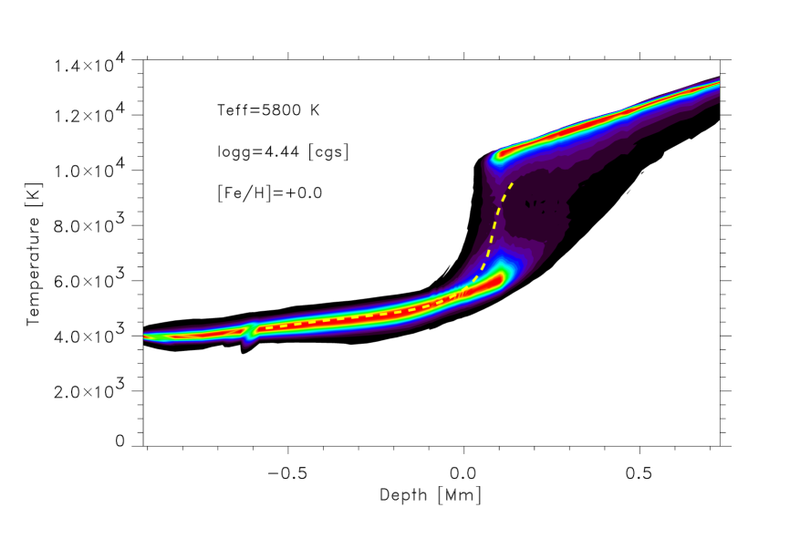
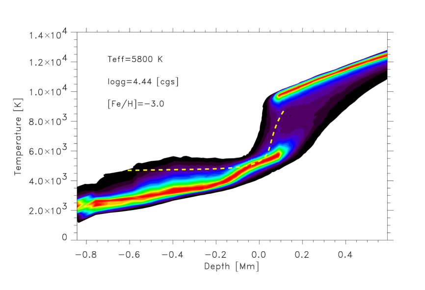
Figure 1: The resulting temperature distribution in the upper part of 3D hydrodynamical convection simulations of the Sun (upper panel) and a metal-poor ([Fe/H] $=-3$) Sun (lower panel). Also shown are the predictions from the corresponding theoretical 1D marcs model atmospheres (dashed lines). The zero-point for the depth-scale corresponds roughly to the continuum optical depth unity. Note the much cooler 3D temperatures in the optically thin layers in the metal-poor star but the rough agreement at solar metallicity (see text for discussion).

In order to obtain a realistic atmospheric structure, it is crucial to have the best possible input physics, and properly account for the energy exchange between the radiation field and the gas. The adopted equation-of-state is that of Mihalas et al. (1988), which includes the effects of ionization, excitation and dissociation. The continuous opacities come from the Uppsala package (Gustafsson et al. 1975 and subsequent updates) while the line opacities are from Kurucz (1998, private communication). The 3D radiative transfer is solved at each time-step under the assumptions of local thermodynamic equilibrium (LTE, $S_{\lambda}=B_{\lambda}$) and opacity binning (Nordlund 1982). The assignment of the original 2748 wavelength points into the different opacity bins follows from detailed monochromatic radiative transfer calculations of the 1D averaged atmospheric structure. The opacity binning thus includes the effects of line-blanketing in a manner reminiscent of opacity distribution functions.

It is important to realise that the simulations contain no free parameters which are tuned to improve the agreement with observations. The adoption of the numerical and physical dimensions of the simulation box is determined by practical computional time considerations, the need to resolve the most important spatial scales and the wish to place the artificial boundaries as far as possible from the region of interest. It has been verified that the resulting atmospheric structures are insensitive to the adopted effective viscosity at the current highest affordable numerical resolution (Asplund et al. 2000a). The input parameters discriminating different models are the surface gravity log $g$, metallicity [Fe/H] and the entropy of the inflowing material at the bottom boundary. The effective temperature of the simulation is therefore a property which depends on the entropy structure and evolves with time around its mean value following changes in the granulation pattern.

The 3D hydrodynamical model atmospheres described above have sofar been performed for solar-type main sequence and subgiant stars (e.g. Nordlund & Dravins 1990; Asplund et al. 1999; Asplund & García Pérez 2001; Allende Prieto et al. 2002). The most profound differences with predictions from theoretical 1D hydrostatic models occur for low-metallicity stars, as first shown by Asplund et al. (1999). In 1D, the presence of spectral lines causes surface cooling and backwarming (e.g. Mihalas 1978), which translates to a shallow temperature gradient for metal-poor stars. In reality however, the radiative equilibrium which is enforced in 1D model atmospheres is not necessary fulfilled. Instead the temperature in the optically thin atmospheric layers is determined by a competition between two opposing effects: radiative heating by absorption of photons in spectral lines and expansion cooling of overshooting upflowing material due to the density stratification. At solar metallicity the two effects nearly balance, leaving the temperature close to the radiative equilibrium expectations. At low metallicities, however, the lack of lines produces much less radiative heating and consequently the resulting temperature is much below the radiative equilibrium value (Asplund et al. 1999), as shown in Fig. 1. At [Fe/H] $=-3$, the difference between 1D and 3D predictions can exceed 1000 K, which obviously can have a dramatic impact on spectral features sensitive to those cool layers, such as molecular and low excitation lines as well as minority species.

Further details of the 3D hydrodynamical model atmospheres are available in Stein & Nordlund (1998), Asplund et al. (1999, 2000a,b) and Asplund & García Pérez (2001).

3 3D spectral line formation

The 3D hydrodynamical model atmospheres described in the previous section form the basis for the 3D spectral line formation calculations. The original 3D hydrodynamical simulations which includes deep, extremely optically thick layers are interpolated to a finer depth scale which extends only down to log $\tau_{\rm Ross}\approx 2.5$ prior to the spectral line calculations for improved numerical accuracy. At the same time, the simulations are interpolated to a coarser horizontal grid to ease the computational burden. For abundance analysis purposes this procedure introduces non-noticable differences ($\leq 0.01$ dex for individual snapshots and less for temporal averages). The concepts of micro- and macroturbulence, which are introduced in 1D analyses in order to account for the missing line broadening, are not necessary in 3D calculations with a self-consistent accounting of Doppler shifts arising from the convective motions.

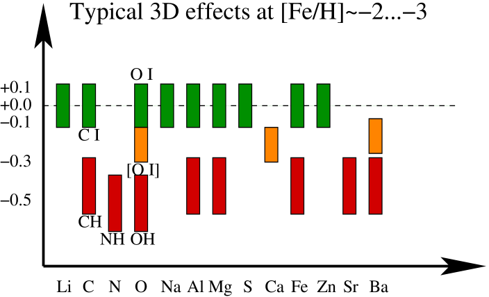
Figure 2: Schematic representation of the expected 3D LTE effects for different elements for $T_{\rm eff}=5800-6200$ K stars with [Fe/H] $\simeq-2$; although not quantitatively investigated here stars with different parameters are expected to show qualitatively similar 3D effects. While many elements apparently are insensitive to the employment of 3D model atomspheres, some species can be quite vulnerable due to their temperature sensitivity, in particular molecular lines (e.g. CH, NH, OH) and low excitation lines. For example, while standard 1D analyses yield accurate results for Fe ii lines, Fe i lines tend to significantly overestimate the Fe abundances. Note that these estimates are based on 3D LTE calculations, while several species may well show significant departures from LTE.

For the spectral line formation calculations presented here the simplifying assumption of LTE has been made, implying that the level populations are determined by the Saha and Boltzmann distributions. With the source function thus known it is then straightforward, albeit computationally intensive, to solve the 3D radiative transfer equation for a number of simulation snapshots before spatial and temporal averaging of the resulting flux profiles. All in all, a single temporally and spatially averaged flux profile in 3D correspond most of the time to $N_{\rm t}*N_{\rm x}*N_{\rm y}*N_{\rm angles}*N_{\lambda}\ga 10^{8}$ 1D radiative transfer calculations. In addition, each 3D profile is normally computed for at least three different abundances to enable interpolation to the requested line strength. Even then, such 3D LTE line calculations are achievable on current workstations thanks to efficient numerical algorithms. Recently, methods enabling even detailed 3D non-LTE line formation for large model atoms have been designed (Botnen & Carlsson 1999) and applied to abundance analyses for Li (Kiselman 1997: Uitenbroek 1998; Asplund et al. 2003a) and O (Asplund et al. 2003b). The near future will doubtless see many more such studies for more elements and 3D model atmospheres.

In order to investigate the possible impact of the new generation of 3D hydrodynamical model atmospheres on globular cluster research, I have selected a number of species and lines which are often used to infer the chemical compositions of globular cluster stars: Li i, C i, O i, [O i], Na i, Mg i, Al i, S i, Ca i, Fe i, Fe ii, Zn i, Sr ii, Ba ii, CH, NH, and OH lines. The 3D LTE line formation calculations were performed for solar-like ($T_{\rm eff}\simeq 5800$ K, log $g=4.4$) and turn-off stars ($T_{\rm eff}\simeq 6200$ K, log $g=4.0$) of varying metallicities ([Fe/H] $=0.0,-1.0,-2.0,-3.0$), as well as for a few 3D models corresponding to specific stars (Procyon, HD 140283, HD 84937, G64-12). Unfortunately, no 3D models are yet available for giants although work towards achieving this goal is ongoing. As mentioned above, no microturbulence enters these 3D calculations. To facilitate an estimation of the 3D effects on derived abundances, corresponding calculations were carried out with the same code using 1D marcs model atmospheres (Asplund et al. 1997), adopting in all cases $\xi_{\rm turb}=1.0$ km s^-1.

4 Results and discussion

Fortunately, several elements appear little, if at all, affected by the employment of 3D hydrodynamical model atmospheres instead of classical 1D hydrostatic models, as shown in Fig. 2. In particular, lines of Li i (in 3D non-LTE), C i, O i, Na i, S i, Fe ii, and Zn i, as well as several Mg i and Al i lines, are essentially immune to the choice of model atmospheres ($\Delta{\rm log}\epsilon<0.1$ dex).

The bad news, however, is that as expected in metal-poor star minority species (e.g. Fe i), low excitation (e.g. Mg i 517 nm, Al i 394 nm, Sr ii 421 nm, Ba ii 455 nm) and all molecular lines tend to significantly over-estimate the abundances by $\geq 0.3$ dex when relying on 1D model atmospheres. The reason for these differences is the much lower temperatures in the optically thin layers at low metallicities. It should be noted, however, that the use of 3D models have recently caused a significant downward revision even of the solar C, N and O abundances (e.g. Asplund et al. 2003b) due mainly to the presence of temperature inhomogeneities in 3D.

As a consequence of the above-mentioned findings, it is clear that globular cluster metallicities should be based on Fe ii lines (see also Kraft & Ivans 2003). In addition, the observed O-Na, Al-Mg, C-N anti-correlations are robust features of globular clusters as are the large cluster abundance variations. While absolute abundances based on molecular lines can be highly misleading, isotopic abundance ratios are not significantly affected.

It should be emphasized, however, that the above estimates are based only on 3D LTE calculations. In some cases there may also be significant 3D non-LTE effects, which may diminish the overall net effects of the new 3D model atmospheres for some species (e.g. Li i, Asplund et al. 2003a) while aggrevate them for others (e.g. O i, Asplund et al. 2003b). Detailed 3D non-LTE calculations for additional elements can be expected for the future, which would finally place the abundance analyses of late-type stars on a firm footing.