Low light level CCDs and visibility parameter estimation

Abstract

Recently, low light level charge coupled devices (L3CCDs) capable of on-chip gain have been developed, leading to sub-electron effective readout noise, allowing for the detection of single photon events. Optical interferometry usually requires the detection of faint signals at high speed and so L3CCDs are an obvious choice for these applications. Here we analyse the effect that using an L3CCD has on visibility parameter estimation (amplitude and triple product phase), including situations where the L3CCD raw output is processed in an attempt to reduce the effect of stochastic multiplication noise introduced by the on-chip gain process. We establish that under most conditions, fringe parameters are estimated accurately, whilst at low light levels, a bias correction which we determine here, may need to be applied to the estimate of fringe visibility amplitude. These results show that L3CCDs are potentially excellent detectors for astronomical interferometry at optical wavelengths.

1 Introduction

Optical interferometry requires the detection of an interference fringe pattern generated when starlight collected by separated apertures is recombined with a spatially or temporally modulated optical path difference (OPD). If the total distance travelled by the two beams of light is equal, or the OPD is a whole number of wavelengths, constructive interference will result in an intensity maxima. Likewise, if the OPD is an odd number of half wavelengths, destructive interference results in an intensity minima. In a typical interferometer, intensities are measured for a range of OPDs, with the OPD differing by a distance of several wavelengths about the zero OPD. Spatial and temporal modulation of the OPD can both be used by optical interferometers, for example the Amber instrument on the VLTI (spatial modulation, Robbe-Dubois et al. (2000)) and the COAST (temporal modulation, Baldwin et al. (1999)). An oscillating signal or fringe pattern results, the contrast and phase of these fringes providing information about the source, including the source diameter and shape, and, when the light is combined using three or more apertures, information about asymmetry within the object. The entire fringe must be sampled within a few times the time-scale of atmospheric perturbations (typically 10 ms in the optical regime), resulting in low signal intensities, and for all but the brightest stars the signal is very faint. To date, the faintest reported optical measurement using a separate element interferometer is an object with visible magnitude of about 8.5 (I magnitude 6.1) (Haniff et al., 2000). Increasing the sensitivity of interferometers is therefore essential if they are to be used to observe a wide range of scientific sources. One way of doing this is to observe over a wide range of wavelengths, allowing a greater light throughput. However, to maintain a useful coherence length, the bandwidth of light on any detector element must be kept small, requiring independent detection of many different wavelengths (spectroscopic detection). This will require at least a one dimensional array of detector elements, which may be expensive and fragile if conventional photon counting detectors (APDs and PMTs) are used.

CCDs ought to be ideal detectors for spectroscopic interferometry because they are stable devices available in large-format arrays, allowing one CCD to replace many single element detectors. However, their major shortcoming is readout noise, i.e. the additional signal added at the on-chip output amplifier where the photo-electrons are counted. A typical interferometer can require CCD readout rates of up to and above 1 MHz since there will be many spectral channels, and each of these must be sampled many times within an atmospheric coherence time. Currently, the best noise level achieved using standard CCDs at these readout rates is typically 10 $\mathrm{e}^{-}$ (Jerram et al., 2001). Signal levels lower than this are then swamped by noise.

Low light level CCDs (L3CCDs) provide a solution to this problem, with an on-chip gain amplifying the signal prior to the on-chip readout amplifier (Jerram et al., 2001), resulting in a sub-electron effective readout noise. This, combined with the high quantum efficiency (QE) of L3CCDs (up to 90 percent), which compares favourably with the QE of APDs (Takeuchi et al., 1999), makes them prime candidates as interferometric detectors. Being array detectors they can be used for spectroscopic detection allowing greater use of the available light, but they do have the disadvantage of introducing an additional source of noise due to the stochastic multiplication process. However for one application, we have shown (Basden et al., 2003) that the magnitude of this noise can be reduced if the L3CCD output signal is treated in the correct way, by thresholding.

In this paper we investigate the use of L3CCDs for interferometric fringe detection. In most situations we find that no bias correction is required to estimate fringe parameters correctly. In some cases, a correction is necessary when estimating visibility amplitude but we provide this correction here. We also develop a suitable treatment allowing unbiased estimation of bispectrum (closure) phase.

The layout of the paper is as follows. In section 2 we present a background to interferometric fringes and the use of L3CCDs, as well as our modelling techniques. In section 3 we present results and our conclusions are summarized in section 4.

2 Interference and L3CCDs

2.1 Introduction to interferometric fringe production

In interferometry, the raw image we obtain is an interferometric fringe pattern, which will show a periodic intensity variation due to either spatial or temporal OPD modulation depending on the type of interferometer. An expression for a general interferometric fringe pattern is given by Scott (1997) (Fig. 1) although for the purposes of this paper we use a simplified version ignoring atmospheric effects, and assuming a monochromatic signal (Eq. 1).

Once a fringe pattern has been recorded, it is useful to obtain the visibility amplitude and (for space based interferometers) visibility phase. If three or more separate apertures have been used, it is possible to measure the bispectrum (or closure) phase.

Figure 1: Example of a simplified fringe pattern with a maximum visibility amplitude of 0.5. The enveloping shape of this fringe pattern is due to a finite signal bandwidth, $\Delta\lambda/\lambda=0.2$ in this case.

2.1.1 Typical light levels

The typical light levels required for measurement by an interferometer are very low, which is why conventional CCDs with higher readout noise are not acceptable as interferometric detectors. For example, observation of a sun-like star with a lossless interferometer at a distance of 1 kpc, with two telescopes of size 1 m diameter, a single pixel detector with a sampling rate of 5 kHz, with a bandpass of 30 nm centered at 700 nm, and a detector with 50 percent quantum efficiency would produce an average detected signal of about 0.7 photons per detector pixel per readout from the interference fringe. It is therefore essential that an interferometric detector must be able to detect individual photons if anything other than bright sources are to be observed.

2.2 L3CCD multiplication noise

The on-chip multiplication process in an L3CCD is stochastic and introduces extra noise into the output signal of the L3CCD before readout, in addition to the Poisson noise due to the detected photons. This reduces the signal-to-noise ratio (SNR) of the raw output by up to $\sqrt{2}$. By processing the raw measured output (Basden et al., 2003) we can reduce the effect of this stochastic noise at low light levels, the reduction depending on the processing strategy that we choose. Increasing the SNR of the L3CCD output signal then allows us to improve our estimate of interferometric visibilities.

We use the processing strategies suggested by Basden et al. (2003) which were developed for photometric applications, namely the “Analogue”, “PC” and “PP” thresholding strategies which are defined as follows:

Analogue:

The L3CCD output is divided by the mean gain.

Photon counting, PC:

If the L3CCD output signal is above some noise threshold, it is assumed to represent one photon.

Poisson probability, PP:

Thresholds are placed at the positions where the L3CCD output probability distribution for a given mean input of $n$ (integer) Poisson photons crosses with the output distribution for a mean input of $n+1$ Poisson photons.

Additionally we here explore a further thresholding strategy denoted as “Uniform”, defined as follows:

Uniform:

Places the L3CCD output signal into evenly spaced thresholds, the spacing being dependent on the mean light level (estimated from the fringe), chosen such that on average, at a given light level, we will estimate the mean photon input correctly. This allows us to make better use of the fringe data. Further details of this thresholding strategy are given in appendix A.

2.3 Numerical models

We investigate the effect of using an L3CCD both with and without processing of the raw output for a range of visibility amplitudes and light levels, categorizing the performance of L3CCDs as interferometric detectors, particularly in the estimation of visibility amplitude and bispectrum (closure) phase. Any additional bias introduced to these measurements by the multiplication process needs to be determined. In this paper we investigate the effect of L3CCDs using Monte-Carlo simulation as follows:

1. Multiple realizations of different fake interferometric fringes were generated.

2. Poissonization of the fringe signal was simulated.

3. The L3CCD stochastic multiplication process on the Poissonized signal was simulated.

4. The simulated L3CCD output was processed using techniques known to reduce the noise introduced by the multiplication process (i.e. Uniform, PP, PC).

5. The effect of these processing strategies on fringe visibility estimation (visibility amplitude and phase, and bispectrum phase) was investigated using standard methods, and checked to see whether the estimates were the same as when using a perfect Poissonian detector.

The interference fringe pattern is modelled assuming a two element interferometer, using the following expression,

$$I_{\mathrm{j}}=\mu\left[1+V\cos\left(2\pi\mathrm{j}m/M+\phi\right)\right]$$ (1)

where $I_{\mathrm{j}}$ is the intensity of the fringe signal in the $\mathrm{j^{th}}$ pixel, for a fringe with a mean intensity $\mu$ and visibility amplitude $V$, with phase $\phi$. The fringe extends over an array of size $M$ pixels ($M=256$ in our case) and contains $m$ whole wavelengths within this array, so that we are not affected by aliasing when Fourier transforming. In our calculations, we ensured that there were always more than eight samples between adjacent peaks of the fringe, so that they were well sampled. Poisson photons with mean intensity $I_{\mathrm{j}}$ were then produced from the theoretical fringe for a given OPD, giving the fringe as it would appear to a detector before multiplication and readout. By modelling the behaviour of the L3CCD multiplication register using a Monte-Carlo simulation following Basden et al. (2003), the effect of L3CCDs on visibility parameter estimation was investigated.

2.4 Visibility amplitude estimation

It is well established (Walkup & Goodman, 1973) that the mean power spectrum (square of the Fourier transform) of an interference fringe averaged over many realizations will yield a DC peak with height $N^{2}$ (where $N$ is the mean number of detected photons in a single fringe), a peak at a position corresponding to the fringe modulation frequency, and a white noise background due to Poisson noise and L3CCD multiplication noise, as shown in Fig. 2. In the case of a two element interferometer considering only photon noise, an unbiased estimate of the visibility amplitude (Walkup & Goodman, 1973) is obtained using

$$|V|=2\sqrt{\frac{E[D^{(2)}(u)]-b}{E[D^{(2)}(0)]-b}}$$ (2)

where $E[D^{(2)}]$ is the power spectrum of the fringe measured at the modulation frequency, $u$, or DC, and $b$ is the noise background level. L3CCD multiplication noise may introduce a bias to the estimator depending on the output thresholding strategy and light level.

In some cases, detector imperfections can introduce a slope to the noise background (Perrin, 2003). However, we have established that these effects are not relevant when using an L3CCD and so we do not consider such effects here.

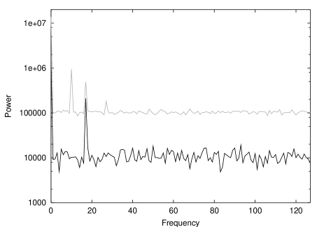
Figure 2: Sample powerspectra of interference fringes produced from L3CCD simulations. The lower (black) trace is produced by a two element interferometer with a mean light level of 1 photon per pixel, and a visibility amplitude of 0.75 from the addition of 20 fringe powerspectra. The upper (grey) trace is produced by a three element interferometer with a mean light level of one photon per pixel, and visibility amplitudes of 0.75, 0.5 and 0.25 from the addition of 200 fringe powerspectra. The white noise background can be seen clearly, and shows that the multiplication process does not alter the slope of this noise.

Walkup & Goodman (1973) give estimates for the number of photon detections that are required to measure the visibility amplitude of a fringe to a specified accuracy. To measure a visibility amplitude $V$ to a SNR of $\mathcal{R}$ in the photon limited case, we require

$$N=\frac{2\mathcal{R}^{2}}{V^{2}}$$ (3)

total signal detections. We therefore generate fringes and sum the power spectra until the total number of Poisson photon detections allows us to reach the required SNR (in our case 50). We then use the summed power-spectrum to estimate the visibility amplitude. We investigate visibility amplitudes between $0.02-1$ at mean light levels between $0.01-20$ photons per pixel, chosen in the range where Basden et al. (2003) find L3CCD output thresholding has a positive effect on the SNR.

2.5 Visibility phase estimation

The visibility phase is meaningful only for space based interferometers, since atmospheric perturbations render it meaningless unless the phase introduced by the atmosphere is known. It is estimated from the phase of the Fourier transform at the fringe modulation peak. When averaging multiple realizations of the fringe pattern, we average the complex value of the peak, not just the phase. This ensures that we give the correct weighting to each individual value, dependent on the number of photons detected.

2.6 Bispectrum phase estimation

When light from at least three apertures is combined at different (non-redundant) OPD modulation frequencies, we can use the detected signal to retrieve some of the phase information by summing together the phases, cancelling the relative phase introduced by the atmosphere. To model this we use a simplified model of the generalized fringe pattern given by Scott (1997). The fringe power spectrum will contain three signal peaks and a DC peak as shown in Fig. 2 (top trace). The bispectrum phase is estimated from the phase of the average complex bispectrum product, with a bias correction that must be applied at low light levels. A suitable correction to apply to the measured bispectrum in the case when detection is governed solely by photon noise is given by Wirnitzer (1985):

$$<Q^{\left(3\right)}\left(u,v\right)> = E\left[D^{\left(3\right)}\left(u,v\right)\right]+c_{1}N$$

$$-c_{2}E\left[|D^{(2)}\left(u\right)|^{2}+|D^{(2)}\left(v\right)|^{2}\right.$$

$$\left.\;\;\;\;\;+|D^{(2)}\left(-u-v\right)|^{2}\right]$$

where $c_{1}=2$, $c_{2}=1$, $<Q^{\left(3\right)}\left(u,v\right)>$ is the unbiased estimate for the bispectrum and $E\left[D^{\left(3\right)}\left(u,v\right)\right]$ is the expected triple product of the fringe (the product of the Fourier transform of the data evaluated at the three signal peaks). We now evaluate the phase of $Q^{\left(3\right)}\left(u,v\right)$ instead of the photon noise biased value of $D^{\left(3\right)}\left(u,v\right)$, with $u$ and $v$ corresponding to the different fringe frequencies, $D^{(2)}(u)$ representing the fringe power spectrum, and $N$ being the total photon count. Eq. 2.6 shows that unlike the power spectrum, the photon bias introduces both constant and frequency dependent terms into the bispectrum.

If the form of the noise is not Poissonian, as is the case when using an L3CCD, a different bias correction may be required. We are able to use results from Pehlemann et al. (1992) to determine the bias correction for the case when we use the raw L3CCD output, obtaining $c_{1}=6$ and $c_{2}=2$. The details, which involves considering the L3CCD output probability distribution, are discussed in appendix C.

If we do not know the detector statistics, it may still be possible to obtain an unbiased estimation of the bispectrum phase. To do this, we used the data to compute $c_{1}$ and $c_{2}$ in Eq. 2.6. This technique relies on Eq. 2.6 being the correct model for the form of the bias correction, and assumes that the power spectrum can be written as

$$E[D^{(2)}(u)]=c_{PS,0}<J^{(2)}(u)>+c_{PS,1}$$ (5)

where $c_{PS,0}$ and $c_{PS,1}$ are scalar coefficients, and $<J^{(2)}(u)>$ is the average power spectrum of the normalized high-light-level (unbiased) fringe.

The coefficients $c_{1}$ and $c_{2}$ were obtained by evaluating the bispectrum at frequencies $u,v$ chosen such that other terms disappear. We give further details in appendix C, and such a scheme was initially proposed by Pehlemann et al. (1992). The form of the power spectrum assumed by this scheme is not always correct, though since differences will be small, we attempted to use this scheme to estimate the bispectrum phase. In most circumstances we find that a correction can be found.

2.7 Theoretically predicted visibility amplitude bias

If we use PP or Uniform thresholding strategies on the L3CCD output we will introduce a systematic bias into our visibility amplitude estimations at some light levels since we place different weightings on fringe minima and maxima. We can get an understanding of how to treat this by considering a theoretical model of the L3CCD output probability distribution as given by Basden et al. (2003):

$$P(x)=\sum_{n=1}^{\infty}\frac{\exp{(-\mu)}\mu^{n}x^{n-1}\exp{(-x/g)}}{n!(n-1)!g^{n}}$$ (6)

where $g$ is the mean gain, $\mu$ is the mean light level and $x$ is the number of electrons at the L3CCD output after multiplication. We can therefore find the estimated light level $I$ in terms of the true light level $\mu$ for any thresholding strategy by writing

$$I=\sum_{a=1}^{\infty}a\sum_{x=f_{a-1}}^{f_{a}}P(x)$$ (7)

where the $a^{\mathrm{th}}$ threshold boundary is represented by $f_{a}$ and $P(x)$ is given above.

The classical definition for visibility is

$$V=\frac{I_{\mathrm{max}}-I_{\mathrm{min}}}{I_{\mathrm{max}}+I_{\mathrm{min}}},$$ (8)

at a given light level $\mu=\left(I_{\mathrm{max}}+I_{\mathrm{min}}\right)/2$ and true visibility $V$. The bias in the estimated visibility amplitude can then be determined, and so corrected, giving us an unbiased estimate for visibility amplitude. We expect our visibility estimate $V_{\mathrm{e}}$ to be equal to:

$$V_{\mathrm{e}}(\mu,V)=\frac{\sum_{a,x,n}aS(x,n)\left(W_{+}-W_{-}\right)}{\sum_{a,x,n}aS(x,n)\left(W_{+}+W_{-}\right)}$$ (9)

with

$$S(x,n) = \frac{\mu^{n}x^{n-1}\exp{(-x/g)}}{n!(n-1)!g^{n}},$$

$$W_{\pm} = \exp(\mp\mu V)(1\pm V)^{n}$$

$$I_{\mathrm{max}} = \sum_{a,x,n}aS(x,n)W_{+}$$

where the summation is over $n=1\rightarrow\infty$, $x=f_{\mathrm{a-1}}\rightarrow f_{\mathrm{a}}$ and finally $a=1\rightarrow\infty$. We have used this theoretical model alongside our Monte-Carlo simulations to verify the predictions we make.

In a similar way, we can compute the visibility amplitude bias when using a single threshold. Since we interpret any signal as a single photon, at a given true light level $\mu$ we measure the mean light level to be $1-\exp(-\mu)$. The true light level at the fringe maxima and minima is given by $I_{\pm}=\mu(1\pm V)$, and so inserting this into the expression for visibility gives

$$V_{e}=\frac{\exp(-\mu)[\exp(\mu V)-\exp(-\mu V)]}{2-\exp(-\mu)[\exp(\mu V)+\exp(-\mu V)]}$$ (10)

where the symbols are as before.

3 Accuracy of fringe parameter estimation

We separate our analysis into three light level regimes, which allows us to apply different L3CCD output thresholding strategies as appropriate for maximum reduction of the noise introduced by the L3CCD multiplication process. Our light level regimes are chosen according to:

Low light levels:

Much less than one photon per pixel per readout ($<0.1$ photons per pixel).

Intermediate light levels:

Between about $0.1-20$ photons per pixel per readout.

High light levels:

More than 20 photons per pixel.

Read noise and gain were found to have little effect on the visibility estimations, provided the mean gain was significantly greater than the read noise as found by Basden et al. (2003). If this was not the case, then the L3CCD output signal was dominated by noise, leading to inaccurate visibility estimation.

We find that all of the L3CCD output thresholding strategies leave the mean power spectrum of the fringe with a flat background. The height of this background is determined by the variance of the signal and in a Poisson case it is equal to the number of photons detected (which is also the variance). When using an L3CCD analogue processing strategy, we find that the background level is twice the height of that from a pure photon noise case as expected since the signal variance is double that of the Poisson case. Similarly, with a single threshold we find that the background level is lower than in the pure photon case by an amount in agreement with the reduction in signal variance. Multiple thresholding strategies give a background level above the pure photon case and below the analogue case, the height depending on light level, in agreement with the variance of the signal (Basden et al., 2003) which is dependent on the light level.

3.1 Visibility amplitude estimation at low light levels ($<0.1$ photons per pixel)

As described by Basden et al. (2003), if the mean light level is low (much less than one photon per pixel per readout) then it is most probably that either one or zero photons will land on a pixel during an exposure. At the L3CCD output we will then have either a relatively large signal corresponding to one photon, or a small signal, just due to noise from the electronic readout amplifier. We can therefore use a PC thresholding strategy treating every signal above a noise level as representing one photon and operating the L3CCD in photon counting mode. We find that the visibility amplitude estimations are unbiased for all visibilities provided the light level is kept low, as shown in Fig. 3 (d).

Figure 3: Plots showing visibility amplitude estimates when using an L3CCD as a function of light level (mean photons per pixel), for visibilities of 1, 0.75, 0.5, 0.2, 0.1, 0.05 and 0.02, with points representing Monte-Carlo simulation results (SNR 50), and curves being theoretical. (a) Results when using an analogue thresholding strategy. In this case no bias is evident. (b) and (c) Showing results when using a uniform thresholding strategy without and with a correction required to estimate amplitude correctly. (d) Showing results using a PC thresholding strategy. Here we see that this cannot be used at light levels greater than about $0.1-0.5$ photons per pixel. (e) and (f) Showing visibility amplitude estimates when using a PP thresholding strategy, before and after correction for visibility amplitude bias respectively.

A uniform thresholding strategy will lead to the same results, since at low light levels it is virtually identical to a PC thresholding strategy. Similarly using an analogue strategy (the raw output), though requiring about twice as many detections to achieve the same SNR due to a larger excess noise factor (Basden et al., 2003), will also provide unbiased visibility estimation. A PP thresholding strategy also provides an unbiased estimate for visibility.

As the light level increases, using a single threshold (PC strategy) causes us to lose estimation accuracy, since there is an increased probability of two or more photons being detected in any given pixel. These signals will be interpreted as a single photon event, and so the fringe maxima will be underestimated more than the fringe minima. Visibility amplitude will be underestimated, and at high light levels will tend towards zero. Other thresholding strategies are then more appropriate.

3.2 Visibility amplitude estimation at intermediate light levels ($0.1-20$ photons per pixel)

At intermediate light levels, we cannot use a single threshold processing strategy as coincidence losses are large. However, we can still reduce the excess noise introduced by the multiplication process by thresholding the L3CCD output signal.

3.2.1 PP and uniform thresholding

We can threshold the L3CCD output signal into predetermined thresholds which are chosen to minimize the excess noise factor introduced by the stochastic multiplication process, for example using the PP thresholding strategy (Basden et al., 2003). Alternatively, we can use the raw data from a fringe to estimate the mean light level. We can then use this along with our knowledge of the mean gain to improve our input prediction, estimating the most likely value of the photon input by choosing appropriate thresholds taking into account the mean light level (appendix A). For any given pixel, the number of photon events may be estimated incorrectly, though on average we will estimate correctly. At low signal levels, we will estimate correctly most of the time, minimizing the dispersion introduced by the multiplication process. As the light level increases, we will lose accuracy progressively (Basden et al., 2003) until there is no advantage in thresholding over using the raw L3CCD output.

Using the PP or Uniform thresholding strategies at light levels between about $0.1-10$ photons per pixel will introduce a small bias to the estimated visibility amplitude. We find that this bias is greatest at light levels of about two photons per pixel, and that here the estimated visibility is just over 80 percent of the true visibility. This is independent of the mean gain, provided the gain is well above the readout noise. An explanation for this bias is given in appendix B, and we find that our Monte-Carlo simulations agree with the theoretically prediced bias (section 2.7). We find that a simple bias correction can be applied according to

$$V_{\mathrm{cor}}\approx\frac{V_{\mathrm{e}}}{V_{\mathrm{e}}^{5/2}\left(1-h(\mu)\right)+h(\mu)}$$ (11)

where $h(\mu)=1-\mu^{3/4}\exp(-\mu/3)/5$ for a mean light level $\mu$ photons per pixel, with $V_{\mathrm{e}}$ representing the biased visibility estimated from the thresholded data, and $V_{\mathrm{cor}}$ being the corrected visibility amplitude. It is important to note that this is only an approximation generated by fitting to the data, though it allows the visibility amplitude to be estimated to about two percent accuracy, i.e. the visibility will be estimated to within $(1\pm 0.02)V_{\mathrm{true}}$. A more accurate bias correction can be estimated by considering the L3CCD output probability distribution, though this requires analytical treatment to compute it.

Monte-Carlo simulation results before the application of the simple bias correction, along with the variation of Eq. 9 and Eq. 10 with $\mu$ and $V$ are shown in Fig. 3 (b), (d) and (e) for the uniform, PC and PP thresholding strategies. Fig. 3 (c) and (f) show the visibility amplitude estimates after the simple bias correction has been applied. We find that the visibility bias is very similar for both the uniform and PP thresholding strategies.

3.2.2 Raw output

Using the analogue processing strategy provides an unbiased estimate for visibility, since we are not weighting the data in any way. This would seem to be a big advantage, except that the SNR can be reduced by a factor of up to $\sqrt{2}$ when compared with other thresholding strategies. We therefore recommend the use of this processing strategy at these light levels in all cases where there is ample SNR. Visibility amplitude reproduction is shown in Fig. 3 (a).

3.3 Visibility amplitude estimation at high light levels

At high light levels, there is no real advantage in thresholding the L3CCD output as this does not improve the SNR, and so an analogue processing strategy should be used, treating the L3CCD output as that from a conventional CCD. Visibilities (amplitude and phase) will be estimated with no additional bias.

3.4 Phase

The visibility phase estimate from a fringe produced by a two element interferometer is unbiased in all of the previously mentioned readout modes (section 2.2) at any light level. It is only fringe peak height, and not position of the fringe that is altered by thresholding the raw L3CCD output, and so the L3CCD has no effect on the visibility phase estimation.

The spread in a phase measurement estimated from many fringes is given by Buscher (1988) as:

$$\alpha=\frac{\sqrt{<\sin^{2}\epsilon>}}{\sqrt{n}<\cos\epsilon>}$$ (12)

where $\epsilon$ is the deviation of the phase estimate from the true phase in each fringe pattern, and $n$ is the number of phase measurements (fringes). We find that $\alpha$ generated by our simulations agrees well with the theoretical SNR $\alpha^{-1}=NV^{2}/2$ (Walkup & Goodman, 1973), when the excess noise factor introduced by the L3CCD multiplication process after thresholding is taken into account. An example from our simulations is shown in Fig. 4.

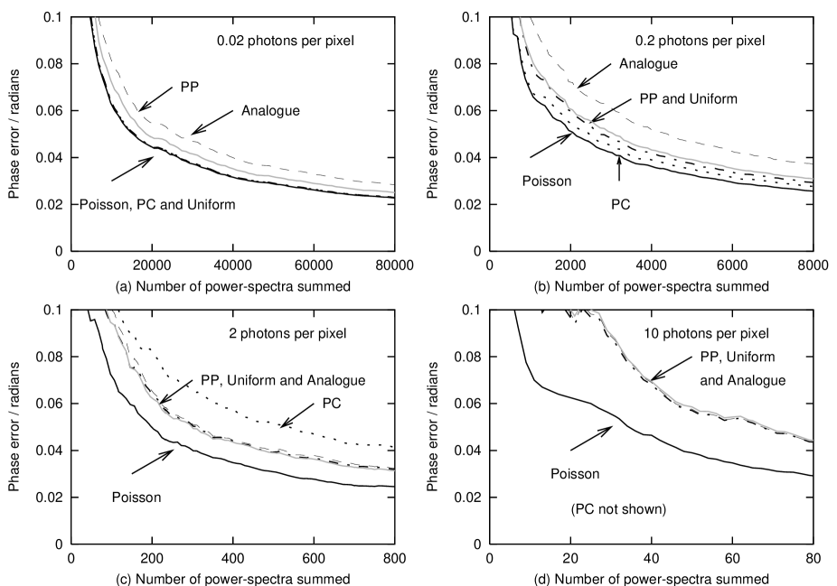
Figure 4: Visibility phase error plotted against the number of fringe patterns recorded and processed when using an L3CCD as a detector. The solid black curves are an example of the phase error that may be obtained when using a perfect detector and closely matches Eq. 3. The dashed curves show the phase error with an L3CCD and an analogue thresholding strategy, the dotted curves for a PC thresholding strategy, the dot-dashed curve for a uniform thresholding strategy and the grey curves for a PP thresholding strategy. All plots are for a visibility amplitude of 0.1, and the mean light level is (a) 0.02 photons per pixel, (b) 0.2 photons per pixel, (c) 2 photon per pixel and (d) 10 photons per pixel. We can see that the analogue thresholding strategy generally requires more photons to reduce the phase error to a given value.

3.5 Bispectrum phase

Our simulations show that when using an L3CCD we are able to estimate the bispectrum phase accurately at mean light levels down to about five photons per pixel when using the standard photon noise bias correction (Eq. 2.6). At lower light levels, the bispectrum phase estimate appears to be biased (Fig. 5). If an analogue or PP thresholding strategy is used with the standard photon bias correction, we find that the estimate of phase tends towards zero as light decreases, even if photometric corrections are applied when using the PP strategy.

In the analogue case, we are able to estimate phase correctly by using the bias correction that we adapted from Pehlemann et al. (1992) (Eq. 2.6 with $c_{1}=6$ and $c_{2}=2$). At very low light levels, a large number of fringe patterns need to be recorded to reduce the SNR to acceptable levels.

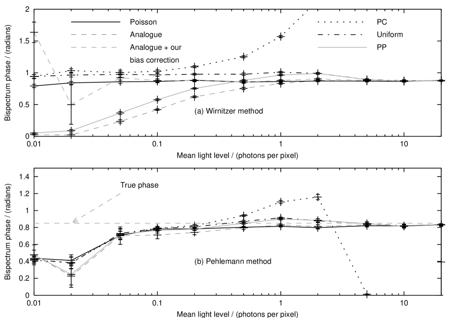
Figure 5: Estimated bispectrum phase when using an L3CCD comparing the performance of different threshold processing strategies (represented by different curves) and estimation techniques (separate plots). (a) We see that using the standard Wirnitzer correction, we are unable to estimate the bispectrum phase at low light levels when using analogue or PP thresholding strategies. However, by using our bias correction, we are able to use the analogue strategy to estimate the phase. We also see that the PC and Uniform thresholding strategies tend to overestimate phase slightly at low light levels. (b) Using the bispectrum phase estimation technique developed by Pehlemann et al. (1992) we are unable to estimate phase accurately at light levels less than about 0.1 photons per pixel. The Poisson curve represents estimation when using a perfect detector, and the true bispectrum phase is 0.85 radians.

Using a uniform thresholding strategy and the standard Wirnitzer (1985) bias correction, we find that the phase is overestimated slightly at low light levels as shown in Fig. 5 (a). A PC thresholding strategy used with the Wirnitzer (1985) bias correction is found to overestimate the phase slightly up to light levels of about 0.2 photons per pixel, above which the estimate tends quickly towards $\pm\pi$ as coincidence losses become large.

The failure of Eq. 2.6 when estimating the phase is due to the L3CCD output probability distribution no longer being Poissonian, which is required for the correction to work correctly. However, by calculating appropriate values for the coefficients in Eq. 2.6 suitable for an analogue processing strategy, we are able to obtain an unbiased estimation of bispectrum phase when using the this processing strategy down to very low light levels.

A similar correction for other L3CCD output processing strategies has not been determined due to the complicated nature of the probability distributions. However, by using a different approach to bispectrum estimation, using the data itself to calculate the bias terms (Pehlemann et al. (1992), section 2.6 and appendix C), we find that we are able to estimate bispectrum phase accurately to light levels down to about 0.1 photons per pixel when using the PP or uniform thresholding strategies. This corresponds to the light levels at which L3CCDs are most likely to be used. Below this, errors in the individual bias terms, and invalid assumptions about the form of the power spectrum reduce the phase estimate below the true value, as shown in Fig. 5 (b).

We recommend the use of the analogue processing strategy and our adapted bias correction as this gives an unbiased estimate of bispectrum phase. Alternatively, if the SNR is low or at very low light levels, we recommend the use of the Uniform thresholding strategy since this is able to reduce the effect of stochastic multiplication noise. The Uniform thresholding strategy will however lead to a slight overestimation of the bispectrum phase by between about $10-20$ percent at the lowest light levels.

3.6 Uncertainties in gain

A knowledge of the mean gain is required when using either the PP or uniform thresholding strategies. If this is not known precisely, threshold boundaries may be placed wrongly. Fortunately, due to the nature of visibility, being composed of both a difference and a ratio (Eq. 8), the effect on the amplitude estimation will be much less than the error in gain.

We find that when using a PP thresholding strategy, the uncertainty in estimated visibility amplitude is inversely proportional to the uncertainty in the gain estimate. If we overestimate the gain by 20 percent, then in the worst case (for low visibilities ($<0.1$) and light levels around two photons per pixel), we will underestimate the visibility amplitude by at most four percent for a PP thresholding strategy, and five percent for a uniform thresholding strategy. For example, if the true mean gain was 1000, but we had estimated it to be 1200, and are trying to measure a true visibility amplitude of 0.05 at a mean light level of 2 photons per pixel, we would estimate the visibility amplitude wrongly by about five percent, i.e. we would estimate the visibility amplitude to be 0.0475.

For visibilities above about 0.1, and mean light levels fainter or brighter than two photons per pixel, the error in visibility is reduced. For PC and analogue thresholding strategies, uncertainties in the mean gain have no effect on visibility estimation.

Typical uncertainties in the gain are of order one percent (Mackay et al., 2001), and so in general there will be negligible uncertainty in the visibility estimate due to this uncertainty. Visibility phase estimates are unaffected by uncertainties in the mean gain.

4 Conclusions

We have investigated the application of L3CCDs to interferometric fringe detection, and the way in which this affects visibility parameter estimation. In doing this, we have introduced an additional (to Basden et al. (2003)) L3CCD output thresholding strategy to enable bispectrum phase estimation at low light levels.

In summary, we find that:

1. L3CCDs can be used for visibility estimation at any light level, though a small bias correction should be applied if a multiple threshold processing strategy is used on the L3CCD output.

2. L3CCD visibility amplitude prediction at high (greater than about ten photons per pixel) and very low (less than 0.1 photons per pixel) photon rates is unbiased for all thresholding strategies.

3. The use of multiple thresholding strategies will introduce a small bias for visibility amplitude at light levels between 0.1-20 photons per pixel.

4. Since the mean gain is typically known to one percent accuracy, the error in visibility amplitude and phase estimation due to this uncertainty will be minimal.

5. At light levels greater than about five photons per pixel, the high-light-level bispectrum phase estimate can be obtained when using L3CCDs. At lower light levels down to about 0.1 photons per pixel, a bias term in the bispectrum phase becomes non-negligible, though this can be corrected by using the data to calculate the bias terms. Below this, a bias correction is still available when the raw L3CCD output is used, giving an unbiased estimate of the bispectrum phase.

6. Using the raw L3CCD output with our adapted bispectrum bias correction, or a uniform thresholding strategy with the standard bias correction allows best bispectrum phase estimation.

Our recommendation is that visibility amplitude and phase estimation at low light levels (less than 0.1 photons per pixel per readout) should be carried out using a single threshold processing strategy on the L3CCD output. At higher light levels, an analogue processing strategy should be used if there is ample signal-to-noise. If the SNR is low, using a multiple thresholding strategy with bias correction will help to improve the visibility estimate. Bispectrum phase estimation should be carried out using either the unthresholded L3CCD output or a uniform multiple thresholding strategy with the corresponding bias correction.

Since L3CCDs provide the most accurate input estimation at low light levels using a single threshold, we recommend that, if possible, they are always used in this regime, increasing the frame rate if necessary to keep the number of photons per pixel low ($<0.1$). We are currently developing a new controller for L3CCDs, allowing pixel rates of up to 30 MHz, which will allow signal levels to be kept low in most interferometric applications.

Appendix A L3CCD uniform thresholding strategy

Basden et al. (2003) provide information about thresholding strategies which can be used to increase the SNR in a signal from an L3CCD. For the purposes of this paper, we here introduce a new thresholding strategy which uses a knowledge of the mean light level to further improve the L3CCD signal SNR. The thresholds are placed with uniform separations, the separation being dependent on light level, chosen so that the mean photon flux is estimated correctly.

A.1 Determining uniform threshold separations

When using L3CCDs for interferometric signal detection, we are able to obtain additional information which will allow us to develop a more accurate thresholding strategy. Since we make measurements of the interference signal over a fringe, we are able to estimate the mean light level within this fringe. We can then use this knowledge along with our knowledge of the mean gain to set the thresholds. Such a thresholding strategy is therefore dependent on the light level and so is only useful when an estimate of this can be obtained reliably in advance. We use a uniform threshold step size (with threshold boundaries being uniformly spaced) sized such that the mean thresholded output signal will be equal to the mean input (though we will not always threshold correctly for each event). We then interpret an L3CCD output signal falling between the $n^{\mathrm{th}}$ and $n+1^{\mathrm{th}}$ threshold as representing $n$ photons.

The probability of obtaining an output $x$ electrons from the multiplication register of an L3CCD with a mean (Poisson distributed) input, $\mu$, is given by (Basden et al., 2003):

$$P(x)=\sum_{n=1}^{\infty}\frac{\exp{(-\mu)}\mu^{n}x^{n-1}\exp{(-x/g)}}{n!(n-1)!g^{n}}$$ (13)

where $g$ is the mean gain and $\mu$ is the mean light level.

Thresholding this signal can improve the noise statistics. We can represent this by

$$P(a)=\sum_{x=f_{a-1}}^{x=f_{a}}P(x)$$ (14)

where $P(a)$ is the probability that a signal is put into the $a^{th}$ threshold, which has boundaries determined by $f_{a}$.

The expected output is then

$$\overline{a}=\sum_{a=1}^{\infty}aP(a).$$ (15)

If we require a thresholding scheme which is able to predict photon flux accurately without any additional corrections, we require the threshold boundaries to be dependent on light level. We equate the above equation to the mean light level, $\mu$, using the threshold boundaries as our degree of freedom. If we wish to have uniformly spaced boundaries ($f_{a}=aT$ for threshold step size $T$), we can express this as

$$\mu = \frac{\exp{\mu}}{g}\sum_{n=1}^{\infty}\left\{\frac{\mu^{n}}{n!(n-1)!}\right.$$ (16)

$$\times\left.\sum_{a=1}^{\infty}\left[a\sum_{x=(a-1)T}^{x=aT}\left(\frac{x}{g}\right)^{n-1}\exp(-x/g)\right]\right\}$$

which should be satisfied by solving $T$ for a given $\mu$.

A good approximation for the theoretical threshold step size at light levels greater than about 0.1 photons per pixel, $T$, is given by

$$T\approx g\left(1+\frac{1}{2\mu^{3/4}}\right)=g\left(1+\frac{g^{3/4}}{2x^{3/4}}\right)$$ (17)

for gain $g$, and mean light level $\mu=x/g$ measured in expected photons per pixel per readout estimated from an L3CCD output of $x$ electrons. At light levels less than about 0.1 photons per pixel it results in a larger threshold size than the ideal, though this is not problematic since at these light levels we are effectively using a large single threshold size, and input estimations are almost identical to those using a PC thresholding strategy.

Using this thresholding strategy, the excess noise factor as defined by Basden et al. (2003) is unity at low light levels, so the SNR scales as $\sqrt{n}$. This is because the step sizes here are large, and so we make correct predictions most of the time. As the light level increases, the excess noise factor tends towards $\sqrt{2}$, the SNR scaling as $\sqrt{n/2}$ (as with the analogue case), halving the effective quantum efficiency of the L3CCD.

For cases where the mean light level can be estimated in advance of thresholding, this processing strategy leads to an improvement over the PC threshold strategy, being applicable at any light level, and results in an increased SNR over the analogue and PP strategies at low light levels, where the improvement is most welcome. It also has the advantage that no additional correction should be made after the event to preserve flux, since it is defined to estimate flux correctly.

A.2 Errors in threshold step size

If the light level or gain are not known precisely, errors may be made when choosing the threshold step size. If the threshold step size is too small, we overestimate the photon count, while if it is too large, we underestimate.

It is straightforward to show that the error in threshold step size depends on the error in gain and light level as:

$$\left(\frac{\Delta T}{T}\right)^{2} = \left(\frac{\Delta g}{g}\right)^{2}+\frac{9}{16}\left(\frac{\Delta\mu}{\mu}\right)^{2}$$ (18)

$$= \frac{25}{16}\left(\frac{\Delta g}{g}\right)^{2}+\frac{18}{16}\frac{1}{m^{3}n}$$

where $\Delta$ represents the uncertainty in a measurement, and the second equality is valid if the mean light level $\mu$ is calculated from $m$ averaged raw L3CCD outputs, each containing a mean of $n$ photons with a SNR of $\sqrt{n/2}$ due to the Poisson and multiplication processes. We can usually expect to know the mean gain to about one percent (Mackay et al., 2001), and so this error is the limiting factor when $m^{3}n\ga 10000$, for example $n=0.0005$ when $m=256$. We can therefore usually expect to be able to choose our threshold step size with an accuracy equal to that in the mean gain.

At high light levels, the fractional error in prediction is proportional to the fractional error in threshold step size. At low light levels, there is less of a dependence since the thresholds are widely spaced, and signals usually fall within the first threshold.

Appendix B Multiple threshold visibility amplitude bias

If we use multiple thresholding on the L3CCD output we will introduce a systematic bias into our visibility amplitude estimations, though we can counter for this effect since we can determine the bias. The reason for this bias is now discussed.

B.1 PP thresholding

When we use a PP thresholding strategy, to estimate the flux correctly we must apply a correction according to (Basden et al., 2003)

$$I_{\mathrm{e}}/I_{\mathrm{r}}\approx\left[1+0.7\exp(-I_{\mathrm{e}}/3)\right].$$ (19)

with subscripts e and r corresponding to estimated and real values respectively. Since this correction depends on the light level, we are therefore biasing our visibility amplitude estimation since fringe minima will have a different weighting (requiring a different correction) than fringe maxima. Our estimate of visibility amplitude will therefore be biased.

We are able to verify this by considering the definition of visibility amplitude, $V=\frac{I_{+}-I_{-}}{I_{+}+I_{-}}$ where $I_{\pm}$ is the intensity at the maximum and minimum of the fringe. Since $1\leq I_{\mathrm{e}}/I_{\mathrm{r}}\leq 1.7$ (Basden et al., 2003), we can further approximate Eq. 19 to

$$I_{\mathrm{e}}\approx I_{\mathrm{r}}\left[1+0.7\exp(-I_{\mathrm{r}}/3)\right].$$ (20)

Therefore, using our estimated flux with $I_{\mathrm{r\pm}}=\mu(1\pm V_{\mathrm{r}})$ for mean light level $\mu$, and inserting into the definition of visibility amplitude, we will obtain an estimate ($V_{\mathrm{e}}$) of the true visibility $V_{\mathrm{r}}$) equal to:

$$V_{\mathrm{e}}\approx\frac{2V_{\mathrm{r}}+0.7\left[f_{+}\exp\left(-\mu f_{+}/3\right)-f_{-}\exp\left(-\mu f_{-}/3\right)\right]}{2+0.7\left[f_{+}\exp\left(-\mu f_{+}/3\right)+f_{-}\exp\left(-\mu f_{-}/3\right)\right]}$$ (21)

where $f_{\pm}=1\pm V_{\mathrm{r}}$. We find that this agrees very closely with our calculation using the probability distributions, Eq. 9.

B.2 Uniform thresholding

If we use a uniform thresholding strategy, then since we are able to measure the mean intensity ($\mu$ photons per pixel) of an interference fringe we use this information to set the threshold step size. However, for visibility V, the fringe intensity will actually vary from a maximum of $\mu(1+V)$ to a minimum of $\mu(1-V)$. At these points our threshold step sizes will be wrong. At a minimum of intensity, the threshold step size chosen from the mean light level will be too small leading to an overestimation of signal, while at intensity maxima the threshold step size will be too large resulting in an underestimation. The combined effect is to underestimate the visibility.

B.3 Low and high light levels

Visibility amplitude bias correction is not be required for mean light levels below about 0.1 photons per pixel, and above about 10 photons per pixel. At the lowest light levels, we will generally only be using the first one or two thresholds, and every photon event will have the same chance of falling into these. At higher light levels, we find that the bias in our visibility amplitude estimation will tend towards zero, leading to correctly estimated visibility amplitude.

Appendix C Bispectrum phase bias estimation

C.1 Unbiased bispectrum phase estimation: Method I

Pehlemann et al. (1992) have studied photon bias compensation of both power spectrum and bispectrum estimation, and derive a method for correcting this. They assume that an image is made from individual photons, each of which may have a different peak intensity, $a_{j}$. We can relate this to the L3CCD output, using the L3CCD output probability distribution. The total expectation value $E[D^{(2)}(u)]$ of the power spectrum of a data set is given by

$$E[D^{(2)}(u)]=c_{PS,0}<J^{(2)}(u)>+c_{PS,1}$$ (22)

where $c_{PS,0}=\overline{N}^{2}\overline{a}^{2}$ and $c_{PS,1}=\overline{N}\overline{a^{2}}$ are scalar coefficients, and $<J^{(2)}(u)>$ is the average power spectrum of the normalized high-light-level (unbiased) fringe. We find that this expression can be applied to the L3CCD raw output since it has this form. However, when using other L3CCD thresholding strategies, this expression is not strictly true, though we do indeed get a flat noise background, $c_{PS,1}$.

The total expectation for the bispectrum, $E[D^{(3)}(u,v)]$ is given by Pehlemann et al. (1992) as

$$E[D^{(3)}(u,v)] = c_{BS,0}<J^{(3)}(u,v)>+c_{BS,2}$$ (23)

$$+ c_{BS,1}\left(<J^{(2)}(u)>+<J^{(2)}(v)>\right.$$

$$+\left.<J^{(2)}(-u-v)>\right)$$

where $c_{BS,0}=\overline{N}^{3}\overline{a}^{3}$, $c_{BS,1}=\overline{N}^{2}\overline{a}\overline{a^{2}}$, $c_{BS,2}=\overline{N}\overline{a^{3}}$ are scalar coefficients and $<J^{(3)}(u,v)>$ is the desired average bispectrum of the normalized high-light-level (unbiased) fringe.

Since we know that the probability distribution for the L3CCD output given a single photon input (Basden et al., 2003) is $P(x)=g^{-1}\exp(-x/g)$, we can calculate the coefficients as:

$$c_{PS,0} = \overline{N}^{2}g^{2}$$

$$c_{PS,1} = 2\overline{N}g^{2}$$

$$c_{BS,0} = \overline{N}^{3}g^{3}$$

$$c_{BS,1} = 2\overline{N}^{2}g^{3}$$

$$c_{BS,2} = 6\overline{N}g^{3}$$

where $g$ is the mean gain. When using the analogue thresholding strategy, we simply divide the L3CCD output by $g$. This allows us to write

$$\overline{N}^{3}<J^{(3)}(u,v)> = E[D^{(3)}(u,v)]+6\overline{N}$$ (24)

$$- 2\left(E[D^{(2)}(u)]+E[D^{(2)}(v)]\right.$$

$$\left.+E[D^{(2)}(-u-v)]\right)$$

from which we can obtain an unbiased estimate of the bispectrum phase.

C.2 Unbiased bispectrum phase estimation: Method II

If we are not easily able to calculate the probability distribution for $a$, we can estimate the required correction terms using our data. To do this, we evaluate the bispectrum at many frequencies chosen so that we can obtain the required coefficients one at a time.

1. By choosing two frequencies, $f_{1}$ and $f_{2}$ such that $f_{1},f_{2}\neq u,v,u+v$ where $u$, $v$ and $u+v$ are the frequencies at which the peaks appear in the power spectrum, we can see that $E[D^{(3)}(f_{1},f_{2})]=c_{BS,2}$, and so obtain an estimate for $c_{BS,2}$.

2. Provided $u\neq v$ and $u\neq 2v$ we evaluate the bispectrum at $f_{1}=f_{2}=u,v,u+v$. At these frequencies, $<J^{(3)}(f_{1},f_{2})>=0$ and so the bispectrum here evaluates to $c_{BS,2}+2c_{BS,1}<J^{(2)}(f_{1})>+c_{BS,1}<J^{(2)}(2f_{1})>$.

3. Using our power spectrum (Eq. 22) we can estimate $c_{PS,0}<J^{(2)}(u)>=E[D^{(2)}(u)]-c_{PS,1}$, obtaining $c_{PS,1}$ from the flat noise background.

4. We are now able to estimate $c_{BS,1}/c_{PS,0}$ from the previous two steps:

   $$\frac{c_{BS,1}}{c_{PS,0}}=\frac{E[D^{(3)}(u,u)]-c_{BS,2}}{2E[D^{(2)}(u)]-3c_{PS,1}}$$ (25)

5. The unbiased bispectrum phase can then be obtained at $f_{1}=u$ and $f_{2}=v$, since this is independent of $c_{BS,0}$.

References

- Baldwin et al. (2001) Baldwin J. E., Tubbs R. N., Cox G. C., Mackay C. D., Wilson R. W., Anderson M. I., 2001, AA 368, L1-4
- Baldwin et al. (1999) Baldwin J. E., Boysen R. C., Haniff C. A., Lawson P. R., Mackay C. D., Rogers J., St-Jacques D., Warner P. J., Wilson D. M. A. and Young J. S., 1998, Current status of COAST. In R. D. Reasenberg, editor, Astronomical Interferometry, volume 3350 of Proc. SPIE, p. 736. Kona, Hawaii
- Basden et al. (2003) Basden A. G., Haniff C. A. and Mackay C. D., 2003, MNRAS in press
- Buscher (1988) Buscher D. F., 1988, PhD Thesis, Univ. Cambridge
- Haniff et al. (2000) C. A. Haniff Baldwin J. E., Boysen R. C., George A. V., Buscher D. F., Mackay C. D., Pearson D., Rogers J., Warner P. J., Wilson D. M. A., and Young J. S., 2000, Proc. SPIE 4006, COAST: the current status, Interferometry in Optical Astronomy, p. 627
- Jerram et al. (2001) Jerram P. Pool, P. J., Bell, R., Burt, D. J., Bowring, S., Spencer, S., Hazelwood, M., Moody, I., Catlett, N. and Heyes, P. S., 2001, Proc. SPIE 4306, p. 178
- Mackay et al. (2001) Mackay C. D., Tubbs R. N., Bell R., Burt D., Jerram P. and Moody I., 2001, Proc. SPIE 4306, p. 289
- Matsuo et al. (1985) Matsuo K., Teich M., Saleh B., 1985, IEEE Transactions on electron devices, Vol. ED-32, No. 12
- Monnier et al. (1999) Monnier J. D., Tuthill P. G., Lopez B., Cruzalebes P., Danchi W. C., Haniff C. A., 1999, ApJ 512, 351-361
- Pehlemann et al. (1992) Pehlemann E., Hofmann K. H. and Weigelt G., 1992, AA 256, 701-714
- Perrin (2003) Perrin G., 2003, AA 398, p. 385
- Robbe-Dubois et al. (2000) Robbe-Dubois S., Antonelli P., Beckmann U., Bresson Y., Gennari S., Lagarde S., Lisi F., Malbet F., Martinot-Lagarde G., Rabbia Y., Rebattu S., Rousselet-Perraut K. and Petrov R., 2000, in 2000 dais.conf 215R Proc. Darwin and Astronomy p215
- Scott (1997) Scott T. R., 1997, PhD thesis, Univ. Cambridge
- Takeuchi et al. (1999) Takeuchi S., Kim J., Yamamoto Y. and Hogue H. H., 1999, Applied Physics Letters 74, p. 1063
- Walkup & Goodman (1973) Walkup J. F., Goodman J. W., 1973, J. Opt. Soc. Am, 63(4), 399
- Wirnitzer (1985) Wirnitzer B., 1985, J. Opt. Soc. Am. A 2, 14-21