The dependence of the sub-stellar IMF on the initial conditions for star formation

Abstract

We have undertaken a series of hydrodynamical simulations of multiple star formation in small turbulent molecular clouds. Our goal is to determine the sensitivity of the properties of the resulting stars and brown dwarfs to variations in the initial conditions imposed. In this paper we report on the results obtained by applying two different initial turbulent velocity fields. The slope of the turbulent power-law spectrum $\alpha$ is set to $-3$ in half of the calculations and to $-5$ in the other half. We find that, whereas the stellar mass function seems to only be weakly dependent on the value of $\alpha$, the sub-stellar mass function turns out to be more sensitive to the initial slope of the velocity field. We argue that, since the role of turbulence is to create substructure from which gravitational instabilities may grow, variations in other initial conditions that also determine the fragmentation process are likely to affect the shape of the sub-stellar mass function as well. The absence of many planetary mass free-floaters in our simulations, especially in the mass range $1-10$ M_J, suggests that, if these objects are abundant, they are likely to form by similar mechanisms to those thought to operate in quiescent accretion discs, instead of via instabilities in gravitationally unstable discs. We also show that the distribution of orbital parameters of the multiple systems formed in our simulations are not very sensitive to the initial conditions imposed. Finally, we find that multiple and single stars share comparable kinematical properties, both populations being able to attain velocities in the range $1-10$ km s^-1. From these values we draw the conclusion that only low-mass star-forming regions such as Taurus-Auriga or Ophiuchus, where the escape speed is low, might have suffered some depletion of its single and binary stellar population.

1 Introduction

It is of central importance in astrophysics to understand how stars form and which mechanisms shape their properties. In particular, the determination of the origin and functional form of the initial mass function of stars and brown dwarfs (IMF) has become the holy grail of star formation studies. The first statistically accurate derivation of the IMF for field stars (Salpeter 1955) yielded a power-law functional form d$N$/d$log$M $\propto$ M^γ with slope $\gamma=-1.35$, in the range $0.4-10$ M_⊙. Subsequent measurements of the IMF for field stars, which explored a wider range of masses, have confirmed the early results of Salpeter: e.g. Miller & Scalo (1979) approximated the IMF by a half-lognormal distribution, for masses between 0.1 and $\approx 30$ M_⊙, the slope above 1 M_⊙ stars being very similar to Salpeter’s. Kroupa (2001) defined an average or Galactic-field IMF which also had a Salpeter slope above 0.5 M_⊙, but could be better fitted by a slope $\gamma=-0.3$ between 0.08 and 0.5 M_⊙ and $\gamma=+0.7$ in the sub-stellar regime. Finally, Chabrier (2003) found that, as a general feature, the IMF is well described by a power-law form for M $\geq 1$ M_⊙ and a lognormal form below, except possibly for early star formation conditions. There is also evidence (see reviews by Kroupa 2002 and Chabrier 2003) that, within the empirical errors, the IMF of clusters, both open and globular, and young associations such as Taurus-Auriga and Ophiuchus, also resembles closely that of field stars, with perhaps some possible variations at the low-mass end. The lack of clear evidence for IMF variations has raised the possibility that the IMF for stars, at least for the disc populations at z $\sim 0$, might be indeed universal.

The IMF at the sub-stellar regime is by no means so well constrained. Brown dwarfs were not discovered until 1995 (Nakajima et al. 1995; Rebolo, Zapatero-Osorio & Martín 1995), and since then a lot of observational effort has been devoted to pinning down the form of the IMF below the hydrogen burning limit (Delfosse et al. 1999; Burgasser et al. 2000; Kirkpatrick et al. 2000; Leggett et al. 2000). From these studies, Chabrier (2002, 2003) concluded that the number density of Galactic disc brown dwarfs is comparable to that of stars, and that the functional form of the IMF in the sub-stellar regime can be characterised, within the uncertainties, by a lognormal distribution. Recently, however, some results seem to indicate that the sub-stellar IMF might indeed be more sensitive to environmental conditions than the stellar IMF. On the one hand, Jameson et al. (2002) find an IMF slope of $\gamma\approx 0.4$ in the sub-stellar regime of the Pleiades for the mass range 0.02-0.075 M_⊙, Muench et al. (2002) show that the Orion-Trapezium cluster has a brown dwarf fraction of $\approx 30\%$ in the same mass range and Barrado y Navascués et al. (2002) derive a sub-stellar IMF slope of $\gamma\approx 0.6$ for the $\alpha$ Persei cluster; i.e. the Pleiades, Trapezium and $\alpha$ Persei young clusters seem to contain a number of brown dwarfs comparable to that of stars. On the other hand, Luhman et al. (2000) and Briceño et al. (2002) find that brown dwarfs are $2\times$ less frequent in Taurus-Auriga than in Orion, result very similar to that found in the IC-348 cluster by Luhman et al. (2003) and Preibisch, Stanke & Zinnecker (2003).

Theoretically, the investigation of the origin of the IMF is by no means straightforward. First of all it is necessary to model the formation of a large number of stars so that the corresponding theoretical IMF can be meaningfully compared with observations. One of the first such attempts was made by Bonnell and collaborators (Bonnell et al. 1997; 2001), who modelled clouds of gas with stellar seeds randomly placed throughout that yielded a functional form for the IMF in close resemblance to the observed stellar IMF. Bonnell et al. (1997, 2001), as well as Klessen, Burkert & Bate (1998) and Klessen & Burkert (2000, 2001), identified two physical processes that contributed to shape the IMF, i.e. dynamical interactions between protostars and competitive accretion. Gravitationally unstable groups of stellar seeds (or dense cores in the case of Klessen & Burkert simulations) would start off with very small masses and subsequently would grow in mass by accretion, which was dubbed competitive because all seeds/cores attempt to feed from the same gas reservoir. This approach was explored further by Delgado-Donate, Clarke & Bate (2003), who performed a large number of calculations of small-$N$ clouds, set up in a similar manner as Bonnell et al. (1997). They concluded that the IMF at the stellar regime is likely to follow the parent core mass function down to the minimum core mass, just to flatten below where internal processes within each core would be dominant.

A more direct approach has recently been conducted by Bate, Bonnell & Bromm (2003; henceforth BBB), who performed a calculation of the fragmentation and collapse of a 50 M_⊙ gas cloud that fully resolved the opacity limit for fragmentation. This simulation, in which a supersonic turbulent velocity field is initially imposed on the gas, results in the formation of $\approx 50$ stars and brown dwarfs, and demonstrated that the resulting IMF is compatible with current observational measurements. This sort of calculations, however, are very demanding computationally, and a wide range of initial conditions cannot easily be explored. A different approach is needed if the dependence of the functional form of the IMF on different initial conditions (i.e. different star formation environments) is to be studied. In this paper we have taken an alternative approach which is a natural complement to the BBB simulation. We find that by modelling an ensemble of isolated cores of mass 5 M_⊙, we can improve the number of stars formed per CPU hour by a factor 7 compared with the BBB calculation. This economy stems from the fact that by focusing on individual dense cores, we dispense with the computational expense of following the diffuse gas in the BBB simulation. We have performed 10 different calculations in which a turbulent velocity field is initially imposed on the gas. This turbulent field is characterised by a power-law velocity spectrum with slope $\alpha$. We have used a different $\alpha$ ($-3$ and $-5$) for each half of the set of calculations. This way, we expect to asses the sensitivity of the properties of the resulting stars and brown dwarfs to the value of the slope of the initial turbulent spectrum in particular, and to variations in the initial conditions for star formation in general.

We stress that our simulations share the property of the BBB simulation that they resolve the opacity limit for fragmentation (Low & Lynden-Bell 1976; Rees 1976) and that, assuming that fragmentation does not occur at densities greater than those at which the gas becomes opaque to infrared radiation, these calculations are able to model the formation of all the stars and brown dwarfs that, under the initial conditions imposed, can be produced. Our spatial resolution limit for binaries allows us to study a wide range of separations, and the particle numbers we employ allow us to model accretion discs around the protostars which are as long lived as those modelled by BBB.

Our study has four major findings:

• The slope of the sub-stellar IMF is sensitive to the initial conditions imposed on the parent cloud. The $\alpha=-3$ case produces a larger fraction of brown dwarfs than the $\alpha=-5$ case. The stellar IMF does not show such statistically significant variations.

• Few objects with masses below $\approx 0.01$ M_⊙ are formed, despite the minimum fragment mass being $10\times$ smaller. This is due to the high accretion rates typical of very young objects formed out of direct collapse or disc fragmentation. Thus, if a large population of free-floating planetary mass objects exists, two explanations may be suggested: first, the standard values for the opacity limit for fragmentation may need to be revised; and/or second, planetary-mass free-floaters may be formed in quiescent discs at later times when the disc mass is much smaller than that of the central object.

• The pattern of mass acquisition among single and multiple stars is shown not to depend sensitively on the slope of the initial turbulent power spectrum. The distribution of the orbital parameters of multiples systems is similarly weakly dependent on initial conditions.

• Single and binary stars attain comparable velocities, between $1-10$ km s^-1. Higher-order multiples have lower velocity dispersions. The $\alpha=-3$ case is more prolific in high-speed escapers. Low-mass, loose star-forming regions such as Taurus or Ophiuchus might have an overabundance of $N>2$ multiples, as lower-$N$ systems may easily escape the potential wells of these associations.

The structure of this paper is as follows. In Section 2 the computational method and initial conditions applied to our models are described. Section 3 presents a description of the cloud fragmentation process. The results on the IMF are given in Section 4. In Section 5 we discuss the dependence of the properties of multiple stars on the initial conditions imposed. Our conclusions are given in Section 6.

2 Computational method

The calculations presented here were performed using a 3D hybrid SPH $N$-body code, designed to follow the dynamics of the stellar system resulting from the fragmentation and collapse of a cloud of cold gas (Bate, Bonnell & Price 1995). The SPH code is based on a version originally developed by Benz (Benz 1990; Benz et al. 1990). The smoothing lengths of particles are variable in space and time, subject to the constraint that the number of neighbours for each particle remains approximately constant at $N_{\rm neigh}=50$. The SPH equations are solved using a $2^{\rm nd}$-order Runge-Kutta-Fehlberg integrator with individual timesteps for each particle (Bate, Bonnell & Price 1995). Gravitational forces and nearest neighbours are calculated using a binary tree. We use the standard form of artificial viscosity (Monaghan & Gingold 1983) with strength parameters $\alpha_{\rm v}=1$ and $\beta_{\rm v}=2$.

2.1 Equation of state

When the gravitational collapse of a molecular cloud core begins, the density is still low enough to preserve an approximate balance between compressional heating induced by the collapse and cooling by molecular line emission (e.g. Larson 1969). During this stage, the gas temperature $T$ can be considered to remain constant. Once the density $\rho$ reaches a critical value $\rho_{\rm c}$ of $\approx 10^{-13}{\rm g~{}cm}^{-3}$, the gas becomes optically thick to infrared radiation and half the energy released by gravitational collapse is retained as thermal energy: the gas is essentially adiabatic. This critical density defines the so-called opacity limit for fragmentation: for an adiabatic gas, with a ratio of specific heats $\eta=7/5$ (appropriate for diatomic gas), the product ($T^{3}\rho^{-1}$)^1/2 increases with density and, therefore, a given Jeans-unstable collapsing clump quickly becomes Jeans-stable, turning into a pressure-supported object.

This pressure-supported object initially contains a few Jupiter-masses (M_J) and has a radius of $\approx 5$ AU (Larson 1969). Although these objects later undergo another phase of collapse due to the dissociation of molecular hydrogen (Larson 1969), it is thought that they are unable to sub-fragment (Boss 1989; Bate 1998). Thus, the opacity limit sets a minimum fragment mass of a few M_J (Low & Lynden-Bell 1976; Boss 1988; BBB).

To model the opacity limit for fragmentation without performing full radiative transfer, we use an equation of state given by $p$ = $K$ $\rho^{\eta}$, where $p$ is the pressure and $K$ is a measure of the entropy of the gas. The value of $\eta$ changes with density as:

$$\eta=\cases{\begin{array}[]{rl}1,&\rho\leq 10^{-13}~{}{\rm g~{}cm}^{-3},\cr 7/5,&\rho>10^{-13}~{}{\rm g~{}cm}^{-3}.\cr\end{array}}$$ (1)

The gas is assumed to consist of pure molecular hydrogen ($\mu$ = 2), and the value of $K$ is such that when the gas is isothermal, $K$ = $c_{\rm s}^{2}$, with $c_{\rm s}=1.85\times 10^{4}{\rm cm~{}s}^{-1}$ at $T=10$ K. The pressure is continuous when the value of $\eta$ changes.

This equation of state matches closely the relationship between temperature and density obtained by full frequency-dependent radiative transfer models of the spherically-symmetric collapse of molecular cloud cores (Masunaga, Miyama & Inutsuka 1998; Masunaga & Inutsuka 2000). It should model collapsing regions well but where departure from spherical symmetry becomes important (e.g. protostellar discs) it may not model the thermodynamics particularly accurately.

2.2 Sink particles

Once the opacity limit for fragmentation is reached and a pressure-supported fragment is formed, the integration of the SPH equations within that object will merely slow down the calculation, thus preventing us from studying the dynamical evolution of the rest of the cloud. Assuming that fragmentation above the opacity limit is irrelevant, the evolution within a collapsed fragment can be ignored and the object replaced by a sink particle (Bate, Bonnell & Price 1995) of the same mass and momentum. This sink particle is inserted when the central density of the fragment exceeds $\rho_{\rm s}=10^{-10}{\rm g~{}cm}^{-3}$, well above the critical density $\rho_{\rm c}$. Sink particles are point masses with an accretion radius, so that any gas particle that falls into it and is bound to the point mass is accreted. Sink particles interact with the gas only via gravity and accretion. The typical initial mass of a sink particle is $\sim$ a few M_J, as a result of the critical density used for the opacity limit for fragmentation. In the present calculations, the sink’s accretion radius $R_{\rm sink}$ is constant and equal to 5 AU. Therefore, discs around sink particles will be resolved only if their radii $\mathrel{\hbox{\hbox to0.0pt{\lower 2.36806pt\hbox{$\sim$}\hss} \kern-3.00003pt\raise 1.72218pt\hbox{$>$}}}10$ AU.

The gravitational acceleration between two sink particles is Newtonian for $r\geq 4$ AU, but is smoothed within this radius using spline softening (Benz 1990). The maximum acceleration occurs at $r\sim 1$ AU; therefore, this is the minimum binary separation that can be resolved. Sink particles are not permitted to merge.

It is worth noting that although the insertion of sink particles, as any other numerical switch, introduces some error in the calculations (a short-lived structure could have been wrongly identified as a protostellar object), the density at which pressure-supported objects are replaced by sinks is 3 orders of magnitude above the critical density $\rho_{\rm c}$. By then, the collapsed fragment is self-gravitating, centrally-condensed and roughly spherical, and has had some time to interact in that form with its environment, thus being potentially exposed to coalescence or disruption. In practice, most pressure-supported objects formed in these calculations would have collapsed to stellar densities were it not for the insertion of a sink particle.

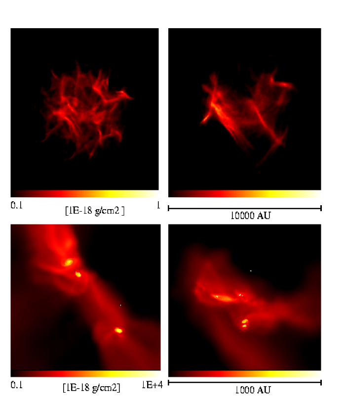
Figure 1: Snapshots of the column density structure of the cloud. On the left for the $\alpha 3$ calculations, on the right for the $\alpha 5$ ones. The upper panels correspond to approximately 10000 yr after the simulations begin. The bottom panels show the state of the cloud some time after the first free fall time, once star-formation has commenced. Column density is plotted in linear scale in the upper panels (where the physical scale is $\approx 10^{4}$ AU), and in logarithmic scale in the bottom panels (here the scale length is $\approx 10^{3}$ AU). Note: higher resolution figure available on request to first author.

2.3 Initial Conditions

We have performed 10 different calculations of the fragmentation of a small-scale, turbulent molecular cloud, each of them under almost exactly the same initial conditions. Each cloud core is spherical, has a mass of 5 M_⊙, a radius of $\approx 10^{4}$ AU, and an initial uniform density of $10^{-18}{\rm g~{}cm}^{-3}$. At the initial temperature of 10 K, the mean thermal Jeans mass is 0.5 M_⊙, i.e. the Jeans number of the cloud is 10. The global free-fall time of the cloud $t_{\rm ff}$ is $\approx 10^{5}$ yr.

We have imposed an initial supersonic turbulent velocity field on the gas, in the same manner as Ostriker, Stone & Gammie (2001) and BBB. We generate a divergence-free random Gaussian velocity field with a power spectrum $P(k)\propto k^{\alpha}$, where $k$ is the wavenumber and $\alpha$ is the power index, which we have set to $-3$ in half of the simulations and to $-5$ in the other half. These values of $\alpha$ bracket the empirical uncertainty in Larson’s velocity dispersion-size relation $\sigma\propto\lambda^{\zeta}$ (Larson 1981). Typical values for $\zeta$ range between $0.35$ and $0.75$ (Larson 1981; Vázquez-Semadeni et al 1997 and references therein), the most quoted value being $0.4$. The exponent $\zeta$ and $\alpha$ are not linearly related. Following Myers & Gammie (1999), we find that $\alpha=-3$ corresponds to $\zeta=0.2$ whereas $\alpha=-5$ corresponds to $\zeta=0.8$. Larson’s mass-size relation M $\propto\lambda^{2}$ is also satisfied by our models (5 M_⊙ in 0.08 pc diameter clouds), although on the high-side of the relation’s scatter. Some of the Lynds clouds in Larson’s original paper, for example, have similar parameters to those used in these models.

Each of the 5 calculations with the same $\alpha$ differ in the values of the random numbers used to generate the velocity field. In turn, for every set of random numbers used to generate a given velocity field, calculations with both values of $\alpha$ have been performed. The velocity field is normalised so that initially it is in equipartition with the gravitational potential energy of the cloud, i.e. initially the cloud is supported by the turbulent motions. The initial root mean square (rms) Mach number of the flow is 3.75. This value of the rms Mach number is in agreement with Larson’s velocity dispersion-size relation, albeit on the high side of the scatter. It must be noted, however, that the turbulent velocity field imposed initially in these calculations is mostly aimed at providing the seeds for the growth of perturbations with a substantial amount of vorticity (as opposed to the models by Delgado-Donate, Clarke & Bate 2003), and can be thought of as a remnant of the previous turbulent fragmentation process (Padoan & Nordlund 2002) that formed the cloud. Consequently, it is not replenished further but permitted to decay freely. Thus, the Mach number will quickly drop to (and remain for the rest of the cloud evolution at) values closer to those observed in molecular cloud cores.

The initial net angular momentum of the cloud is very small. If locked in global solid body rotation, it would account for a value of $\beta$ (the ratio of rotational to gravitational potential energy in the cloud) as low as 10^-3. Yet locally, the angular momentum can be very high, as contained in the vorticity associated with the modes of a divergence-free turbulent field. In principle, these initial conditions do not favour the formation of wide binary stars.

Each cloud is bound by a small external pressure in order to prevent the escape of SPH particles during the first free fall time of the cloud evolution, when the thermal energy contained in the gas is not negligible relative to the cloud gravitational energy. These simulations do not include magnetic fields, as we have tried to isolate a particular hydrodynamical fragmentation problem to characterise the properties of the resulting stellar systems. We have not included in our models any mechanical or radiative feedback mechanism. This may be an appropriate choice, since the maximum stellar mass in these simulations does not exceed 1 M_⊙, whereas the most powerful winds and photoionisation fronts in star-forming regions are produced by much more massive stars.

2.4 Resolution

The local Jeans mass must be resolved throughout the calculation (Bate & Burkert 1997; Truelove et al. 1997; Whitworth 1998), otherwise some of the fragmentation might be artificially suppressed. The minimum Jeans mass M_res occurs at the maximum density during the isothermal collapse phase $\rho_{\rm c}$, and is $\approx 0.0015$ M_⊙ (1.5 M_J). When modelling self-gravitating gas with SPH, a Jeans mass must contain at least $2\times N_{\rm neigh}=100$ SPH particles (Bate & Burkert 1997). Thus, following equation (6) of Bate & Burkert (1997), we need to use $3.5\times 10^{5}$ particles to model a 5 M_⊙ cloud core. In practice, any collapsing gas clump in these simulations contains more SPH particles than M_res, since a clump with a mass of M_res, when compressed, would heat up and subsequently would exceed the Jeans mass: truly pre-stellar clumps must be more massive than M_res to keep collapsing.

Angular momentum transport in accretion discs is also affected by the number of particles used in the simulations. SPH artificial viscosity forces (in particular the $\alpha_{\rm v}$ term) give rise to unrealistically high values of the effective viscosity in accretion discs (Artymowicz & Lubow 1994). The consequence is that, unless many particles (of the order of $10^{5}$) are present in the disc at any given time – which is not the case – the disc dissipates too quickly. This may have an effect on the dynamical interactions between stars and/or brown dwarfs in our models: e.g. a given star-star encounter may well have different outcomes depending on whether it is mediated by discs or not, since the amount of dissipation of the stars’ kinetic energy depends on the amount of disc material they interact with. In addition, since we can only resolve discs which are larger than  10 AU, encounters with impact parameters smaller than 10 AU will not be modelled completely accurately even if they involve stars that still harbour large discs.

Each of the calculations that are discussed in this paper required $\approx 4000$ CPU hours on the SGI Origin 3800 Computer of the United Kingdom Astrophysical Fluids Facility (UKAFF).

3 The evolution of the cloud

The hydrodynamical evolution of the cloud produces shocks which decrease the turbulent kinetic energy that initially supported the cloud. In parts of the cloud, gravity begins to dominate and dense self-gravitating cores form and collapse. These dense cores are the sites where the formation of stars and brown dwarfs occurs. The turbulence decays on the dynamical timescale of the cloud core (as found by MacLow et al. 1998; Stone, Ostriker & Gammie 1998; and BBB, among others), and star formation begins just after 1 to 1.5 global free-fall times $t_{\rm ff}$. The calculations are stopped when 60% of the gas has been accreted (i.e. at 60% star-formation efficiency). In terms of $t_{\rm ff}$ this means that, for the $\alpha$ = $-3$ and $\alpha$ = $-5$ calculations (henceforth $\alpha 3$ and $\alpha 5$) , we follow the evolution of the cloud for $\approx 4t_{\rm ff}$ and $5.5t_{\rm ff}$, respectively (i.e. an average of $\approx 0.5$ Myr). Altogether, at 60% efficiency, the calculations produce 145 stars and brown dwarfs: 85 in the 5 $\alpha 3$ runs, and 60 in the other 5 $\alpha 5$ runs.

The physical scale of the structures formed during the first $t_{\rm ff}$ is markedly different for the two sets of initial conditions. Figure 1 shows four snapshots of the column density structure in the clouds, the upper panels corresponding to $\approx 0.1t_{\rm ff}$. The $\alpha 3$ case is depicted on the left, and the $\alpha 5$ on the right. The formation of filamentary or sheet-like structures is common to both initial conditions. But clearly the $\alpha 5$ case, in which more kinetic power is stored in the long wavelength modes ($\lambda>1000$ AU) of the turbulent velocity field (relative to the $\alpha 3$ case), shows larger coherent structures, and results in a more pronounced expansion of the initial gas spatial distribution. Once a large fraction of the initial turbulent kinetic energy is dissipated via shocks, dense pockets of gas begin to form. The $\alpha 5$ case produces, on average, more dense cores per simulation: from 2 to 3; and these cores are more widely separated than in the $\alpha 3$ case, in which never more than 2 dense cores are formed. The average number of protostars formed in each core varies by a factor of $\approx 2$ depending on the initial conditions used ($\approx 4$ in the $\alpha 5$ simulations and $\approx 7$ in the $\alpha 3$ ones). The formation of the first pressure-supported object also takes longer, on average, for the $\alpha 5$ case. Once the formation of several dense cores has taken place, the subsequent evolution of the cloud and the star formation process inside each core is qualitatively independent of the value of $\alpha$ initially imposed.

All the objects formed in these calculations start off with a mass close to the opacity limit for fragmentation. Subsequently, they grow in mass by accretion. Initially, a pressure-supported object forms within each dense clump, first in isolation but soon surrounded by an accretion disc. Initially the mass of the disc is comparable to, and often greater than the mass of the central object. Thus, the disc is prone to the appearance of gravitational instabilities which, in most cases, result in the fragmentation of the disc into one or more protostellar objects (Bonnell 1994; Bonnell & Bate 1994; Burkert, Bate & Bodenheimer 1997; Whitworth et al. 1995). The formation of this first star generally occurs in the lowest of the local potential minima. Surrounding condensations with slightly lower gas densities form additional stars (e.g. in the filaments whose intersection generated the first dense clump). Both the stars and the residual gas are attracted by their mutual gravitational forces and fall towards each other (see Figure 1, bottom panels). The interactions between the gas and the protostars dissipate some of the kinetic energy of the latter (Bonnell et al. 1997), allowing the stellar objects to rapidly come close to the initial star and its disc-born companions, to form a high-density sub-cluster containing from 2 up to 8 stars: a small-$N$ cluster. This process repeats itself in other parts of the cloud. Subsequently, sub-clusters are attracted to each other and merge to form the final mini-cluster. Thus, the star formation process is hierarchical in nature, as has been vividly illustrated (for a 1000 M_⊙ cloud) by Bonnell, Bate & Vine (2003).

Figure 2: Number of stars $+$ brown dwarfs formed in each calculation. Squares refer to the $\alpha 3$ group, asterisks to the $\alpha 5$ simulations. The solid line represents the mean number of objects (for the combined dataset) and the dashed line the standard deviation of the mean. The initial Jeans number of the clouds is 10.

Star formation is not only localised in space (the sub-clumps) but also in time, i.e. proceeds in bursts (BBB): after one burst occurs, most of the dense gas in the vicinity is exhausted and some time is needed for more gas to be accreted from regions further away. The time sequence of star-forming bursts depends on the local distribution of dense gas and on the number and boundedness of the objects populating the small-$N$ cluster. In most of the simulations the last burst is triggered by the dynamical interactions induced by the last merger, after which the cloud becomes stellar-dominated instead of gas dominated. We have taken special care that all simulations were run until at least 1 $t_{\rm ff}$ after the last star formation event. Thus, we expect to have computed the formation of all the stars and brown dwarfs that could ever have been formed in these clouds, under the initial conditions imposed.

Overall, the $\alpha 5$ simulations form less stars and brown dwarfs than the $\alpha 3$ runs (60 against 85). Stars and, particularly brown dwarfs, form with a higher incidence if small-scale structure is generated during the early evolution of the cloud. In this case multiple fragmentation within a dense core occurs more efficiently. The $\alpha 5$ simulations are characterised by the absence of small-scale structure initially, since there is comparatively much less energy stored in small wavelengths ($\lambda<1000$ AU) initially than in the $\alpha 3$ case. In addition, it is the long wavelength modes that contribute most to prevent the global collapse of the cloud, therefore keeping dense cores away from each other much longer: thus, star formation induced by mergers between small-$N$ clusters occurs also more efficiently in the $\alpha 3$ simulations than in the $\alpha 5$ ones.

The process of fragmentation and collapse out of a turbulent molecular cloud is largely stochastic. Hence, the number of stars and brown dwarfs formed in each individual calculation varies. However, in Figure 2 we show how this number seems to fluctuate around a mean value, which coincides approximately (within a factor of 2) with the initial number of Jeans masses contained in each cloud, i.e. 10. The $\alpha 5$ simulations form an average of $12\pm 3$ stellar objects, for $17\pm 3$ in the $\alpha 3$ group (the error being the standard deviation of the mean). This result seems to suggest that in effect the number of Jeans masses $N_{\rm J}$ may determine, at any rate, the number of objects formed in a collapsing cloud: in principle there is no a priori reason why some of the calculations could not have produced, say, just one star or 50. It remains unclear however, how far-reaching this relation between $N_{\rm J}$ and the number of objects formed is (BBB also form $\approx 50$ objects in an initially 50 $N_{\rm J}$ cloud), and if it is linear or not.

4 Variations in the sub-stellar mass function

Figure 3: Mass functions. On the upper left, we show the mass function derived from the $\alpha 3$ calculations; on the upper right, the same for the $\alpha 5$ initial conditions. On both diagrams three histograms are plotted: the solid, dashed and dotted lines correspond to 60%, 30% and 15% star-formation efficiency (the amount of gas converted into stars) respectively. The dot-dashed line represents the Salpeter IMF. Masses are shown in M_⊙. The bottom panels depict the cumulative mass distributions from both groups of simulations, on the left for 15% efficiency, 60% efficiency on the right. The truncated dashed line marks the mass at which the maximum difference between the two distributions is found. The $\alpha 3$ mass distribution is displayed with diamonds, the $\alpha 5$ one with squares.

In Figure 3 [upper panels] we plot the mass function derived by combining the results from all the simulations of a given $\alpha$. On the left, the $\alpha 3$ case is shown, and the $\alpha 5$ mass function on the right. It can be readily seen that, as mentioned before, the total number of objects formed is lower in the $\alpha 5$ case. In addition, it is apparent that the fraction of brown dwarfs is also lower in the $\alpha 5$ case, for efficiencies higher than 15%: $\approx 30\%$ of all the objects formed in the $\alpha 5$ simulations are brown dwarfs; in contrast, the $\alpha 3$ form almost equal numbers of stars and brown dwarfs. The difference arises most evidently in the 0.01-0.02 M_⊙ bin, in which as many as $\approx 20$ brown dwarfs are located at 60% efficiency in the $\alpha 3$ runs, for only $\approx 8$ sub-stellar objects in the same bin in the $\alpha 5$ simulations. To first order, the transition to the sub-stellar regime is characterised by a flat slope, though the precise trend is different depending on the initial value of $\alpha$. For the $\alpha 5$ group, after a turn over at about 0.4 M_⊙, the mass function decreases (in logM space) and has a cutoff at about 0.01 M_⊙. The $\alpha 3$ mass function displays a similar turn-over point but later declines in the range 0.02-0.4 M_⊙, just to rise again in the 0.01-0.02 M_⊙ bin. A cutoff at $\approx 0.01$ M_⊙ is also seen in this case.

The slope at the high mass end ( $>0.4$ M_⊙) can be compared with a Salpeter power-law. The comparison highlights that stars with masses greater than 1 M_⊙ are underproduced, i.e. the high-mass end does not resemble a Salpeter IMF. This, however, should not be surprising, since all the clouds have an initial mass of 5 M_⊙, i.e. do not follow any distribution of masses as one would expect in a real molecular cloud. Delgado-Donate, Clarke & Bate (2003) showed that the slope of the IMF before the turn-over is likely to be dominated and hence follow the slope of the core/cloud mass function. BBB do find a slope above 0.5 M_⊙ which resembles the Salpeter value, for their simulation of a 50 M_⊙ cloud, in which three entirely independent cores are formed, each with a different mass. Therefore, our mass functions (MFs) must be understood not so much as IMFs, but in essence as the building blocks of such IMF. An IMF could be constructed from our MFs by simply convolving them with a cloud mass function. For this purpose, our mass functions at the high mass end may be better described by an approximate $\gamma=0$ narrow power law in logM space, followed by a quick drop at about 1 M_⊙. This characteristic mass of the upper cutoff depends on the initial cloud mass, the number of objects formed and the efficiency assumed.

In order to build an IMF by means of a convolution of the MFs with a core/cloud mass function we need to make two assumptions, because our MFs are not scale-free. First, some sort of correlation should exist between the initial Jeans number and the initial mass of the cloud so that more massive clouds form more stars. Second, the only mass scale to influence the pattern of mass acquisition at the high mass end within each cloud should be the Jeans mass at the opacity limit for fragmentation and not the initial cloud mass (Bate et al. in prep.). This last assumption is likely to break down at high cloud masses ( $>50$ M_⊙), as enough independent sub-clumps may form so as to yield a mass function readily comparable to the IMF (BBB). For low-mass star-forming regions, however, this should not be a concern. Thus, under these two assumptions, we may consider the high mass end of the mass function per given core mass as being roughly scale-free and thus amenable to be convolved with a cloud mass function. If the slope of the cloud mass function is close to Salpeter’s, the result of the convolution will be an IMF that at the high mass end will resemble closely the observed IMF (see Delgado-Donate, Clarke & Bate 2003).

The bottom panels of Figure 3 show in each diagram the cumulative mass functions for both initial conditions (at 15% efficiency on the left and 60% efficiency on the right). From the cumulative distributions it is possible to perform a Kolmogorov-Smirnov (KS) test and thus calculate the probability $P_{\rm KS}$ of both mass functions being drawn from the same distribution. $P_{\rm KS}$ turns out to be smaller than 0.05 for efficiencies greater than 15%. Thus, at the $2\sigma$ confidence level, the two mass functions appear to be different. However, the mass at which the maximum difference between the two cumulative distributions occurs (and from which the KS probability is calculated) are $\approx 0.05$ M_⊙ and $\approx 0.02$ M_⊙ for the 15% and 60% efficiency cases respectively. [Although large differences are also found in the 60% case at larger masses, this only reflects a property of cumulative distributions: the offset between the two distributions at very low masses is simply carried forward to larger masses]. Therefore, it is the mass distribution in the sub-stellar regime that is responsible for $P_{\rm KS}$ being 0.05. We can conclude then that the stellar mass function is rather insensitive to the different initial conditions imposed, whereas the sub-stellar mass function does depend on the initial slope of the turbulent power spectrum.

Why does the $\alpha 3$ initial condition result in the formation of a higher fraction of brown dwarfs? The fact that the $\alpha 3$ simulations are characterised by having more powerful short wavelength ($\lambda<1000$ AU) turbulent modes than the $\alpha 5$ runs ensures that small-scale structure is more important in the former. Therefore, in the neighbourhood of each collapsing core the gas is highly structured and thus prone to multiple fragmentation. In addition, due to the lack of support in large scales against collapse in the $\alpha 3$ case, the accretion rates on to the dense cores and, in particular, on to the circumstellar discs, is very high, thus making the discs more likely to be gravitationally unstable than in the $\alpha 5$ case. The net result is that in the $\alpha 3$ calculations the number of objects in each small-$N$ cluster is larger (by a factor of $\approx 2$) than in the $\alpha 5$ runs. Consequently a higher fraction of objects are ejected in the $\alpha 3$ case. Low mass components are the prime candidates for being ejected, and once they become unbound or simply bound at large separations, their accretion process is effectively brought to a halt. Therefore, the $\alpha 3$ simulations tend to produce a larger fraction of brown dwarfs than the $\alpha 5$ runs.

In summary, star-forming regions (SFR) which start off with a high degree of substructure at small scales ($<1000$ AU) must be expected to form a large fraction of very low mass objects, and hence render the sub-stellar mass function different to that of looser, less structured SFRs. And this should be so independently of the physical mechanism that drives the formation of such substructure. Thus, by extension, we speculate that the sub-stellar mass function is likely to be rather sensitive to the environment in which star formation takes place, and not exclusively to the slope of the initial power spectrum, as we have shown explicitly here. This possible dependence of the sub-stellar IMF on initial conditions may have already been observed in several star-forming regions. In particular, Briceño et al. (2002) and Preibisch, Stanke & Zinnecker (2003) find that Taurus and IC 348 respectively, have a deficit of brown dwarfs, their fraction relative to stars being $\sim$ a factor of 2 lower than in more massive SFR such as Orion (Muench et al. 2002), the Pleiades (Jameson et al. 2002) or $\alpha$ Persei (Barrado y Navascués et al. 2003).

4.1 Planetary mass free-floaters and the minimum mass for fragmentation

We mentioned previously that the lower cutoff in both mass functions is located at $\approx 0.01$ M_⊙. That is, the characteristic mass at which the number of brown dwarfs drops significantly lies at about 10 M_J. No brown dwarf is found to have a mass lower than $\approx 4$ M_J, and the fraction of brown dwarfs with masses below 10 M_J is smaller than 10%. The position of the lower cutoff in the mass functions is also independent of the choice of efficiency. Only for very short timescales can brown dwarfs be found to have masses close to the minimum resolvable mass.

All the objects in our simulations start with a mass close to the Jeans mass at the critical density $\rho_{\rm c}$, or M${}_{\rm res}\approx 1.5$ M_J. Therefore, the low fraction of planetary-mass brown dwarfs is not only determined by our choice of the critical density $\rho_{\rm c}$ (at which the gas becomes optically thick) but also by some universal process occurring to all collapsed fragments: essentially, the accretion rates during the first years after each protostar forms are very high, high enough so as to allow the accretion of $\approx 10\times$ the initial Jeans unstable mass before dynamical interactions with neighbouring objects become important. Typical values for the accretion rates in our simulations during the first 10 yrs after formation are $\sim 10^{-3}-10^{-4}$ M_⊙/yr. We have checked that the initial accretion rates are not artificially enhanced by a large factor by the inclusion of sink particles in the calculation. An additional simulation in which sink particles have an accretion radius $10\times$ smaller was performed. The accretion rates derived are, on average, only a factor 5 lower, not low enough to prevent the accretion of $\approx 0.01$ M_⊙ in still a very short timescale.

Thus, the detection of a few planetary-mass free-floating objects (PMOs) in the mass range $1-10$ M_J can be readily accommodated within the context of our models. However, if a large population of PMOs exists, two explanations for its origin might be suggested. First, they might form via the same mechanisms at work in our simulations, namely direct fragmentation in filaments or disc fragmentation induced by gravitational instabilities. But then the minimum fragment mass should be $\approx 10\times$ lower than in the present simulations, i.e. the critical density $\rho_{\rm c}$ should be $\approx 100\times$ higher than assumed here. Although this possibility cannot be ruled out, such a high value of $\rho_{\rm c}$ would not be easy to explain in terms of our current knowledge of the thermodynamical processes that determine $\rho_{\rm c}$ (but see Boss 2000).

Second, PMOs may be formed in large numbers in quiescent accretion discs at later times than modelled here (e.g. during the stellar dominated phase of star formation), when the disc mass is much smaller than that of the central object. In this situation, even if gravitational instabilities drive fragmentation in the disc, the fragments will lack a large reservoir of gas from which to accrete substantially, and hence their masses will remain close to the initial fragment mass, i.e. a few M_J. These two possibilities are not mutually exclusive.

5 Weak variations in the properties of multiple stars

Figure 4: Mass functions for the $\alpha 3$ simulations on the left, and the $\alpha 5$ ones on the right. The solid line represents the mass function calculated using all the stars and brown dwarfs formed in each group of calculations, at 60% efficiency. The dashed line histograms only include the inner members (up to a distance of 1000 AU) of multiples systems, while the dot-dashed line histogram represents the mass distribution of unbound single objects (i.e. escapers). Mass is shown in M_⊙.

Delgado-Donate et al. (2003) discussed the properties of the multiple stars resulting from these simulations. Their analysis referred to the combined dataset, regardless of which initial conditions had been applied in each situation. This is justified since the properties of multiples stars, as we will show presently, display a weak dependence on the slope of the initial turbulent velocity spectrum.

5.1 The IMF revisited: companions and singles

Figure 4 shows the mass function derived from each group of calculations: on the left the $\alpha 3$ case and on the right the $\alpha 5$, at 60% efficiency. Overplotted we show the mass distribution of the members of multiple systems up to a separation of 1000 AU (dashed line), and the mass distribution of unbound singles (i.e. escapers; dot-dashed line). Two features are apparent: first, the vast majority of the inner members of a multiple system have high-masses ($0.3-1$ M_⊙), this being the case independently of the initial conditions applied. Second, unbound singles (objects that escaped the cloud after being ejected via a three-body encounter) populate mostly the $0.01-0.1$ M_⊙ range. However, a tail of higher-mass (up to 0.3 M_⊙) escapees can be also found in the $\alpha 5$ case. That is, dynamical interactions do not occur so often in the $\alpha 5$ simulations, and therefore some objects have the chance to accrete to relatively high masses before being ejected from the system. Nonetheless, it is clear that the pattern of mass distribution among singles and multiples is very much the same for both groups of calculations: low-mass singles and high-mass multiple companions.

Notably, the $\alpha 3$ calculations (those in which the number of stars and brown dwarfs are more similar) are characterised by a mass function that can be seen as bimodal, the low-mass peak being made up of single unbound brown dwarfs, and the high-mass peak being populated by the inner members of multiple systems. This pattern of mass acquisition was also found in the small-$N$ clusters simulations of Delgado-Donate, Bate & Clarke (2003). They performed a large number of calculations involving a spherical cloud of gas, initially homogeneous and static, seeded with 5 accreting point masses (sink particles) each, and where the processes of competitive accretion and dynamical interactions could be studied irrespectively of complications such as star-creation and star-disc interactions. They found that the bimodal structure of the mass function per given core could be understood purely as a result of those two processes: repeated three-body interactions leading to ejections and binary hardening; and spherical accretion, which was dubbed competitive because all the stars try to feed from the same, finite, gas reservoir. Given the similarity between the small-$N$ cluster bimodal mass function and the mass function of our $\alpha 3$ simulations, it is tempting to conclude that it is mostly the interaction between many protostars in a relatively small ($<10^{4}$ AU) gas-rich volume that generates this pattern of mass acquisition, regardless of other intervening processes such as the initial turbulent flow structure or subsequent star-disc interactions. In other words, whereas the turbulent flow may determine the number of interactions between the protostars, and their strength (by inducing a more or less compact clustering of a lower or higher number of stars), it is the acting of the dynamical interactions themselves (i.e. a series of stochastic processes leading to continuous restructuring of the internal configuration of multiple systems) in a gas-rich environment what ultimately determines the properties of multiple stars and the overall shape of the IMF below the Salpeter range.

5.2 Orbital parameters

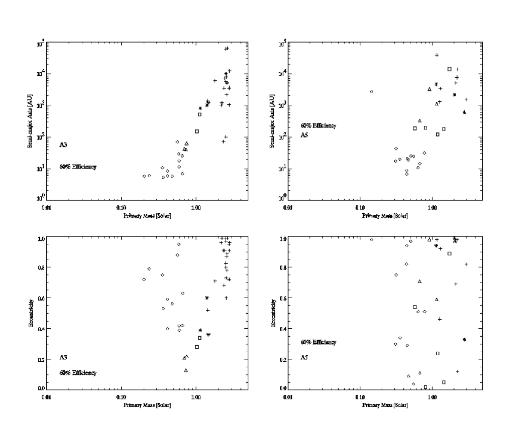
Figure 5: Semi-major axis (in AU) versus primary mass (in M_⊙) on the upper diagrams; eccentricity versus primary mass (in M_⊙) on the bottom ones. On the left, for the $\alpha 3$ calculations, on the right for the $\alpha 5$ calculations. The symbol code is as follows: diamonds represent binaries, triangles triples, squares quadruples, asterisks quintuples, and crosses higher-order multiples. All the plots show results at 60% efficiency. Note: higher-resolution image available on request to first author.

Figure 5 shows the distribution of orbital parameters (semi-major axis $a$ [top panels] and eccentricity $e$ [bottom panels]) versus primary mass, for the $\alpha 3$ calculations (on the left), and the $\alpha 5$ ones, on the right. Figure 5 displays results at 60% efficiency only. The symbol code is as follows: binaries are represented by diamonds, triples by triangles, quadruples by squares, quintuples by asterisks and higher-order multiples by crosses. Both sets of initial conditions result in the formation of multiple systems with similar distributions of $a$ and $e$. The mean separation of binaries is $\approx 10$ AU, lower than observed for G-stars (Duquennoy & Mayor 1991; this is due to the lack of wide pure binaries, as described in Delgado-Donate et al. 2003). Triples, quadruples, etc show an increasingly larger mean semi-major axis, as it would be expected for systems that have a hierarchical or nearly hierarchical configuration. A similar pattern is evident for both groups of simulations, the most important difference between them being the mean $a$ of triples, at $\approx 1000$ AU in the $\alpha 5$ calculations but at $\approx 100$ AU in the $\alpha 3$ ones.

Binary stars can have a wide range of eccentricities, from 0.05 to 0.95. The $\alpha 5$ simulations show a higher incidence of low-eccentricity binaries, probably due to the lower number of dynamical interactions that take place in those calculations, relative to the $\alpha 3$ ones. High-order multiples are characterised by very high values of $e$. These high-order multiples are more frequent in the $\alpha 3$ simulations, simply because many more low mass objects are formed in this case, and it is the lightest members of an unstable multiple that are likely to be thrown to wide orbits after ejection.

Overall, although some differences between the distribution of orbital parameters (as a function of primary mass) for each initial condition can be appreciated, they are not very significant statistically.

5.3 Kinematics

Figure 6: Velocity (in km s^-1) versus primary mass (in M_⊙), at 60% efficiency. On the left, the $\alpha 3$ results; on the right, the $\alpha 5$ results. The symbol code is as in Figure 5, the only difference being the small tilted crosses, which represent unbound single objects.

Figure 6 depicts the distribution of velocities for singles and multiples, versus primary mass (on the left, for the $\alpha 3$ group, and the $\alpha 5$ results shown on the right). The symbol code is as in Figure 5, with the addition of small tilted crosses, which represent unbound singles. Both diagrams show similar trends: first, the highest velocities are attained among singles, but the offset between the mean velocity of singles and that of multiples (binaries and triples specifically) is very small. For all practical purposes, single stars and binaries can be said to define a single kinematical population. A similar result was also found by BBB in their larger cluster simulation. However, high-order multiples such as quadruples or quintuples do have a significantly lower mean velocity. Second, only a minority of objects (mostly low-mass singles) attain speeds close to $\approx 10~{}{\rm km~{}s}^{-1}$. The $\alpha 3$ case is more prolific in high-speed escapers. This should be expected, as the small-$N$ clusters formed in the $\alpha 3$ calculations are denser and, consequently, encounters at shorter distances are more likely.

It must be noted that the number of escapers and their ejection speed may be sensitive to the softening radius applied in this simulations ($\approx 4$ AU). Following Armitage & Clarke (1997), we find that the typical ejection velocity of a very-low-mass star/brown dwarf which suffers an encounter at 4 AU with a stellar binary is $\approx 10$ km s^-1. (To calculate this number we have taken the median mass of escapers and binaries formed in our calculations [0.02 M_⊙ and 0.4 M_⊙ respectively], and assumed a twin binary). This 10 km s^-1 value is substantially higher than the average velocity of escapers in our simulations, indicating that encounters at distances of $\approx 4$ AU cannot be frequent. But particularly in the $\alpha 3$ case, there are some escapers with velocities close to 10 km s^-1. Therefore, in this case, we might be missing some encounters with higher velocities. That is not the case for the $\alpha 5$ simulations.

Two conclusions can be drawn from the two trends mentioned above: first, the majority of low-mass stars and brown dwarfs ever formed in a high-mass SFR like Orion are expected to remain bound: thus, young open clusters should still contain most of their initial brown dwarf population, albeit in the outermost regions due to internal mass segregation. We see a trend, however, for dense SFRs (our $\alpha 3$ simulations) to eject more objects with high velocities than loose SFRs. Second, the role of binary-binary interactions (leading to the ejection of binaries) is determinant in mixing the kinematic properties of single stars and multiples. These interactions could not take place in the simulations of Delgado-Donate, Bate & Clarke (2003) and Sterzik & Durisen (1998), which formed only one binary per cluster, and therefore found that the offset between the velocities of singles and binaries was much larger. Thus, it is only the systems with highest $N$ (quadruples, quintuples, etc…) that remain kinematically distinct. These differences are unlikely to be detected in an actual SFR, since clouds as those we modelled here also move with respect to each other with a velocity of a few ${\rm km~{}s}^{-1}$. But it might be possible that, in loose low-mass associations such as Taurus, some fraction of the single and pure binary population has escaped to the field. This might help to explain why the binary fraction in Taurus is enhanced by a factor of 2 compared to solar-type stars on the main sequence (Ghez, Neugebauer & Matthews 1993; Simon et al. 1995; Köhler & Leinert 1998), and why the companion frequency (the number of companions per stellar system) is the highest of all young SFRs (Duchêne 1999).

6 Conclusions

We have undertaken a series of hydrodynamical simulations of multiple star formation in small molecular clouds. Our approach of modelling 10 independent small clouds of 5 M_⊙ each instead of just one cloud of 50 M_⊙ has allowed us to explore different initial conditions. In this paper we have discussed the effect that different slopes of the power law spectrum of the initial turbulent velocity field has on the properties of the resulting stars and brown dwarfs. Two slopes have been applied, $\alpha=-3$ and $\alpha=-5$, and the other initial parameters (total mass, cloud radius, number of Jeans masses, initial turbulent kinetic energy) have been kept constant. Particular emphasis has been given to the analysis of the mass function of the stars and brown dwarfs formed in these simulations, and its possible variation with initial conditions. It is worth mentioning that the IMFs analysed in this paper are derived directly from the masses of stars actually formed in numerical calculations, as a result of the interplay between turbulence, self-gravity, competitive accretion between protostars and dynamical interactions in unstable multiple systems. In our models, stars and brown dwarfs start off with masses close to the opacity limit for fragmentation (a few M_J) and subsequently grow in mass by accretion. Our approach is different to that of Padoan & Nordlund (2002) who, although they started with isothermal gas and similar inputs of turbulent energy, did not include self-gravity in their simulations nor followed fragmentation down to the opacity limit. They derived an IMF by applying some relations concerning the Jeans mass to the density probability distribution function of compressible turbulence. No actual self-gravitating object (i.e.‘star’) was (or indeed could be) formed in their calculations.

Our main conclusions are:

• The fraction of brown dwarfs (out of the total number of stellar and sub-stellar objects) formed in our calculations is sensitive to the initial slope of the turbulent power spectrum. The brown dwarf fractions produced by the 2 sets of simulations are statistically different at the $2\sigma$ level. The origin of this difference can be explained in terms of the degree of substructure that the different initial conditions are able to generate. In the $\alpha 3$ case, the amount of kinetic energy stored in short-wavelength ($\lambda<1000$ AU) turbulent modes is higher than in the $\alpha 5$ case, and consequently the dense cores in which the cloud fragments remain highly structured even after the decay of turbulence. This results in the formation of more objects per dense core in a more compact configuration, leading to a higher incidence of ejections of low-mass members than in the $\alpha 5$ case. Therefore, we speculate that the shape of the sub-stellar mass function is likely to be sensitive to the degree of substructure present in each SFR (observational hints in this direction have recently been provided by Briceño et al. 2002, Luhman et al. 2003 and Preibisch, Stanke & Zinnecker 2003), independently of the physical process responsible of the generation of such substructure. A KS test applied to the mass functions resulting from each $\alpha$ also demonstrates that the distribution of masses at the stellar regime does not show any significant dependence on the value of $\alpha$. Thus, we conclude that it is the slope of the sub-stellar IMF, rather than that of the stellar IMF, that is likely to be affected by star-formation environmental conditions.

• We find that few brown dwarfs with masses less than $\approx 0.01$ M_⊙ are formed in our simulations. Only 10% of all brown dwarfs have masses in the range $1-10$ M_J, despite the minimum fragment mass being $10\times$ lower. This result is a consequence of the high accretion rates ($\sim 10^{-3}-10^{-4}$ M_⊙/yr) characteristic of the very first years of a protostar’s life, which result in the mass of most of the objects increasing by a factor of 10 in a very short timescale. This timescale is typically shorter than $\sim 100$ yr and therefore the probability that dynamical interactions act to eject the object during that time is almost negligible. Therefore we conclude that although the detection of a few planetary-mass free-floating objects (PMOs) can be accommodated by our models, if a large population of PMOs exists, then other explanations for their origin must be sought. Either the value of the critical density $\rho_{\rm c}$ that determines the minimum fragment mass may need to be revised, and/or PMOs may be formed in large numbers in quiescent discs at later stages than modelled here – in a relatively gas-poor environment –, when the disc mass is much smaller than that of the central object and therefore a large reservoir of gas is not available for the fragment to grow in mass by accretion.

• The pattern of mass acquisition among single and multiple systems is shown not to depend sensitively on the slope of the initial turbulent power spectrum. Likewise, the distribution of orbital parameters (semi-major axis and eccentricity) of the multiples is only weakly dependent on initial conditions.

• Singles and binaries constitute a kinematically homogeneous population (mean velocity dispersion $\sim$ few km s^-1). The offset between the mean velocity dispersion of each group is substantially smaller than found in the simulations of Delgado-Donate, Clarke and Bate (2003), and arises from the mutual interactions between binary systems. High-order multiples ($N>4$) attain significantly lower velocities ($\sim 0.1$ km s^-1), and thus might remain closer to the densest cores of a SFR than higher-speed members. Only a minority of objects (mostly low-mass singles) attain speeds close to $\approx 10{\rm km~{}s}^{-1}$. The $\alpha 3$ case is more prolific in these high-speed escapers, indicating that as expected, dense SFRs eject more objects with high velocities than loose SFRs.

References

- [] Armitage P. J., Clarke C. J., 1997, MNRAS, 285, 240
- [] Artymowicz P., Lubow S. H., 1994, ApJ, 421, 651
- [] Barrado y Navascués D., Bouvier J., Stauffer J. R., Lodieu N., McCaughrean M. J., 2002, A&A, 395, 813
- [] Bate M. R., 1998, MNRAS, 508, 95
- [] Bate M. R., Bonnell I. A., Price N. M., 1995, MNRAS, 277, 362
- [] Bate M. R., Burkert A., 1997, MNRAS, 288, 1060
- [] Bate M. R., Bonnell I. A., Bromm V., 2003, MNRAS, 339, 577 [BBB]
- [] Benz W., 1990, in Buchler J. R., ed., The Numerical Modeling of Nonlinear Stellar Pulsations: Problems and Prospects, Kluwer: Dordrecht, 267
- [] Benz W., Bowers R. L., Cameron A. G. W., Press W., 1990, ApJ, 348, 647
- [] Bonnell I. A., 1994, MNRAS, 269, 837
- [] Bonnell I. A., Bate M. R., 1994, MNRAS, 269, L45
- [] Bonnell I. A., Bate M. R., Clarke C. J., Pringle J. E., 1997, MNRAS, 285, 201
- [] Bonnell I. A., Clarke C. J., Bate M. R., Pringle J. E., 2001, MNRAS, 324, 573
- [] Bonnell I. A., Bate M. R., Vine S. G., 2003, MNRAS, 343, 413
- [] Boss A. P., 1988, ApJ, 331, 370
- [] Boss A. P., 1989, ApJ, 346, 336
- [] Boss A. P., 2000, ApJ, 545, L61
- [] Briceño C., Luhman K. L., Hartmann L., Stauffer J. R., Kirkpatrick J. D., 2002, ApJ, 580, 317
- [] Burgasser et al., 2000, AJ, 120, 1100
- [] Burkert A., Bate M. R., Bodenheimer P., 1997, MNRAS, 289, 497
- [] Chabrier G., 2002, ApJ, 567, 304
- [] Chabrier G., 2003, PASP, 115, 763
- [] Delfosse X., Tinney C. G., Forveille T., Epchtein N., Barsenberger J., Fouqué P., Kineswenger S., Tiphène D., 1999, A&AS, 135, 41
- [] Delgado-Donate E. J., Clarke C. J., Bate M. R., 2003, MNRAS, 342, 926
- [] Delgado-Donate E. J., Clarke C. J., Bate M. R., Hodgkin S. T., 2003, MNRAS, submitted
- [] Duchêne G, 1999, A&A, 341, 547
- [] Duquennoy A., Mayor M., 1991, A&A, 248, 485
- [] Ghez A. M., Neugebauer G., Matthews K., 1993, AJ, 106, 2005
- [] Jameson R. F., Dobbie P. D., Hodgkin S. T., Pinfield D. J., 2002, MNRAS, 335, 853
- [] Kirkpatrick J. D., Reid I. N., Liebert J., Gizis J. E., Burgasser A. J., Monet D. G., Dahn C. C., Nelson B., Williams R. J., 2000, AJ, 120, 447
- [] Klessen R. S., Burkert A., Bate M. R., 1998, ApJ, 501, L205
- [] Klessen R. S., Burkert A., 2000, ApJS, 128, 287
- [] Klessen R. S., Burkert A., 2001, ApJ, 549, 386
- [] Köhler R., Leinert C., 1998, A&A, 331, 977
- [] Kroupa P., 2001, MNRAS, 322, 231
- [] Kroupa P., 2002, Science, 295, 82
- [] Kroupa P., Bouvier J., Duchêne G., Moraux E., 2003, MNRAS, in press, astro-ph/0307229
- [] Larson R. B., 1969, MNRAS, 145, 271
- [] Larson R. B., 1981, MNRAS, 194, 809
- [] Leggett S. K., Geballe T. R., Fan X., Schneider D. P., Gunn J. E., Lupton R. H., Knapp G. R., Strauss M. A., McDaniel A., Golimowski P. A. et al., 2000, ApJ, 536, 35
- [] Low C., Lynden-Bell D., 1976, MNRAS, 176, 367
- [] Luhman K. L., 2000, ApJ, 544, 1044
- [] Luhman K. L., Stauffer J. R., Muench A. A., Rieke G. H., Lada E. A., Bouvier J., Lada C. J., 2003, ApJ, 593, 1093
- [] MacLow M. M., Klessen R. S., Burkert A., Smith M. P., Kessel O., 1998, Phys.Rev.Lett., 80, 2754
- [] Masunaga H., Miyama S. M., Inutsuka S., 1998, ApJ, 495, 346
- [] Masunaga H., Inutsuka S., 2000, ApJ, 531, 350
- [] Miller G. E., Scalo J. M., 1979, ApJS, 41, 513
- [] Monaghan J. J., Gingold R. A., 1983, J. Comput. Phys., 52, 374
- [] Muench A. A., Lada E. A., Lada C. J., Alves J., 2002, ApJ, 573, 366
- [] Myers P. C., Gammie C. F., 1999, ApJ, 522, L141
- [] Nakajima T., Oppenheimer B. R., Kulkarni S. R., Golimowski D. A., Matthews K., Durrance S. T., 1995, Nature, 378, 463
- [] Ostriker E. C., Stone J. M., Gammie C. F., 2001, ApJ, 546, 980
- [] Padoan P. Nordlund A., 2002, ApJ, 576, 870
- [] Preibisch T., Stanke T., Zinnecker H., 2003, A&A, in press
- [] Rebolo R., Zapatero-Osorio M. R., Martín E. L., 1995, Nature, 377, 129
- [] Rees M. J., 1976, MNRAS, 176, 483
- [] Salpeter E. E., 1955, ApJ, 121, 161
- [] Simon M., Ghez A. M., Leinert Ch., Cassar L., Chen W. P., Howell R. R., Jameson R. F., Matthews K., Neugebauer G., Richichi A., 1995, ApJ, 443, 625
- [] Stone J. M., Ostriker E. E., Gammie C. F., 1998, ApJ, 508, L99
- [] Truelove J. K., Klein R. I., McKee C. F., Holliman J. H., Howell L. H., Greenough J. A., 1997, 489, L179
- [] Vázquez-Semadeni E., Ballesteros-Paredes J., Rodríguez L. F., 1997, ApJ, 474, 292
- [] Whitworth A. P., Chapman S. J., Bhattal A. S., Disney M. J., Pongracic H., Turner J. A., 1995, MNRAS, 277, 727
- [] Whitworth A. P., 1998, MNRAS, 296, 442