Superimposed Oscillations in the WMAP Data?

Abstract

The possibility that the cosmic variance outliers present in the recently released WMAP multipole moments are due to oscillations in the primordial power spectrum is investigated. Since the most important contribution to the WMAP likelihood originates from the outliers at relatively small angular scale (around the first Doppler peak), special attention is paid to these in contrast with previous studies on the subject which have concentrated on the large scales outliers only (i.e. the quadrupole and octupole). As a physically motivated example, the case where the oscillations are of trans-Planckian origin is considered. It is shown that the presence of the oscillations causes an important drop in the WMAP $\chi^{2}$ of about fifteen. The F-test reveals that such a drop has a probability less than $0.06\%$ to occur by chance and can therefore be considered as statistically significant.

I Introduction

The recently released WMAP data wmap have confirmed the standard paradigm of adiabatic scale invariant primordial fluctuations hinshaw ; verde . This paradigm can be justified in the framework of inflation and can explain the most important cosmological observations peiris ; saminf . This remarkable success has led the cosmologists to take an interest in more subtle features of the WMAP multipole moments. In particular, recently, many studies have been devoted to the so-called cosmic variance outliers, i.e. points which lie outside the one sigma cosmic variance error outEf ; outCon ; outCline ; outFeng ; TMB ; alain ; huang03 ; Ef . These outliers have been considered as intriguing since the probability for their presence would be very small spergel . So far, all the studies have concentrated on the seeming lack of power at large scales, i.e. on the quadrupole and the octupole outliers. In the literature, two possibilities have been envisaged. In Ref. Ef , it has been argued that the outliers are not a problem at all, the crucial point being the way the probability of their presence is estimated. In Refs. outCon ; outCline ; outFeng ; TMB , it has been envisaged that the outliers could be a signature of new physics even if it has also been recognized in these articles that the cosmic variance could be responsible for their presence. In particular, in Ref. outCon , it has been proposed that the inflationary scale invariant initial power spectrum could be modified by some new physics such that a sharp cut-off at large scales appears while it remains unchanged elsewhere. It has been shown that this can cause a decrease of the $\chi^{2}$ of order $\Delta\chi^{2}\simeq 2-4$ for one additional free parameter given by the scale of the cut-off.

However, as revealed by the Fig. 4 of Ref. spergel , the main contribution to the WMAP $\chi^{2}$ does not come from the large scales but rather from scales which correspond to the first and second Doppler peaks (more precisely, according to Ref. spergel , the three main contributions come from the angular scales $\ell\simeq 120,200$ and $340$). In other words, if the presence of outliers is taken seriously into account, modifications of the standard power spectrum seem to be required on a different range of scales and, in any case, not only at very large scales. In addition, the small scale outliers can be above or below the theoretical error bar and, therefore, the required modifications do not seem to have the form of a systematic lack or excess of power. This naturally leads to the idea that the power spectrum could possess superimposed oscillations. The aim of this article is to study whether this idea has any statistical support. Of course, a physical justification for the presence of oscillations in the power spectrum is needed. Interestingly enough, such a justification exists precisely in the context of the theory of inflation wang ; MB1 ; BM1 and we now discuss this question in more details.

One of the main advantage of the inflationary scenario is that it permits to fix sensible initial conditions. Because the Hubble radius was constant during inflation, the wavelength of a mode of astrophysical interest today was much smaller than the Hubble scale at the beginning of inflation whereas, without a phase of inflation, the same mode would have been a super-Hubble mode. Contrary to the super-Hubble case, the vacuum is defined without ambiguity in the sub-Hubble regime. This state is the starting point of the subsequent cosmological perturbations evolution. This leads to a nearly scale-invariant spectrum for density perturbations, a prediction which is now confirmed to a high level of accuracy wmap ; hinshaw ; verde ; peiris ; saminf .

However, this remarkable success carries in itself a potential problem. In a typical model of inflation, the modes are initially not only sub-Hubble but also sub-Planckian, that is to say their wavelength is smaller than the Planck length $m_{{}_{\mathrm{Pl}}}^{-1}$ MB1 ; BM1 . In this regime, the physical principles which underlie the calculations of the power spectrum are likely not to be valid anymore. This problem is specific to the perturbative approach and does not affect the background model. Indeed, since the energy density of the inflaton field is nearly constant during inflation, we face in fact a situation where the wavelength of the Fourier modes is smaller than the Planck length whereas the energy density which drives inflation can still be well below the Planck energy density. The problem described above mainly concerns the modes of cosmological (still in the linear regime) interest today which are, in the inflationary paradigm, a pure relic of the trans-Planckian regime. It should be added that the scale at which the new physics shows up is not necessarily the Planck length but could be everywhere between this scale and the Hubble radius. In this article we denote the new energy scale $M_{\mathrm{c}}$ and assume that $\sigma_{{}_{0}}\equiv H/M_{\mathrm{c}}$ is a free parameter ($H$ denotes the Hubble parameter during inflation). If the physics is different beyond the scale $M_{\mathrm{c}}$, this should leave some imprints on the spectrum of inflationary cosmological perturbations and therefore modify the Cosmic Microwave Background (CMB) anisotropies wang ; MB1 ; BM1 .

The next question is how to calculate these modifications. Roughly speaking, the calculation of the power spectrum of the fluctuations reduces to the calculation of the evolution of a free quantum scalar field in a time-dependent background. Various methods have been used to model the physics beyond $M_{\mathrm{c}}$ like changing the free dispersion relation MB1 ; BM1 ; N ; LLMU , using stringy uncertainty relations Kempf ; EGKS ; EGKS2 ; KN ; BH ; HS or noncommutative geometry LMMP . Yet another approach has been to assume that the Fourier modes are “created” when their wavelength equals the critical scale $M_{\mathrm{c}}^{-1}$ D ; EGKS3 ; ACT ; AL ; BM03 . A generic prediction, first made in Refs. MB1 ; BM1 , which appears to be independent of the settings used to model the new physics, is the presence of oscillations in the power spectrum (of course, the detailed properties of these oscillations do depend on the model utilized). This can be understood easily. In the standard calculation, initially, the scalar field is just given by an in-going wave. If the evolution proceeds according to the WKB approximation MSwkb , at Hubble scale exit the scalar field will just differ by a phase which will drop out when the power spectrum is calculated. On the other hand, if the WKB approximation is violated at some time before Hubble scale exit or if the modes are created at a fixed length in some $\alpha$-vacuum, then the scalar field will be a combination of on-going and out-going waves. This combination gives the oscillations in the power spectrum. To put it differently, one can say that the existence of a preferred scale plus the standard inflationary theory generically imply a power spectrum given by a nearly scale invariant component plus superimposed oscillations.

The aim of this article is to use the previous generic trans-Planckian prediction as a tool to analyze whether the WMAP multipole moments exhibit oscillations originating from oscillations in the primordial spectrum. It should be stressed again that, in this work, the trans-Planckian effects are only considered as an example of models where oscillations could show up. Indeed, the analysis presented in this article would still be useful for any alternative model which predicts a similar oscillatory pattern.

This paper is organized as follows. In the next section, we briefly recall the standard calculation of the inflationary spectrum when the trans-Planckian effects are taken into account. In Sect. III, we compare the theoretical predictions with the WMAP data. Finally, we discuss the data analysis and give our conclusions in Sect. IV.

II The trans-Planckian power spectra

In this article, we assume that inflation of the spatially flat FLRW spacetime is driven by a single scalar field $\phi_{{}_{0}}(\eta)$. Scalar perturbations of the geometry can be characterized by the gauge-invariant Bardeen potentials $\Phi$ and fluctuations in the scalar field are characterized by the gauge-invariant quantity $\delta\phi$. If $\phi_{{}_{0}}^{\prime}\neq 0$ (a prime denotes derivative with respect to conformal time $\eta$), then everything can be reduced to the study of a single gauge-invariant variable (the so-called Mukhanov-Sasaki variable) defined by MFB $v\equiv a(\delta\phi+\phi_{{}_{0}}^{\prime}\Phi/{\mathcal{H}})$, where $\mathcal{H}=aH$ is the conformal Hubble parameter. In fact, it turns out to be more convenient to work with the variable $\mu_{{}_{\mathrm{S}}}$ defined by $\mu_{{}_{\mathrm{S}}}\equiv-\sqrt{2\kappa}v$, where $\kappa\equiv 8\pi/m_{{}_{\mathrm{Pl}}}^{2}$. Density perturbations are often characterized by the so-called conserved quantity $\zeta$ MS defined by $\zeta\equiv(2/3)({\cal H}^{-1}\Phi^{\prime}+\Phi)/(1+w)+\Phi$, where $w$ is the equation of state parameter. The quantity $\mu_{{}_{\mathrm{S}}}$ is related to $\zeta$ by $\mu_{{}_{\mathrm{S}}}=-2a\sqrt{\gamma}\zeta$, where $\gamma=1-{\mathcal{H}}^{\prime}/{\mathcal{H}}^{2}$. On the other hand, the primordial gravitational waves are described by the transverse and traceless tensor $h_{ij}$, the Fourier transform of which is $\mu_{{}_{\mathrm{T}}}$ (up to a polarization tensor). Both types of perturbations obey the same type of equation of motion, namely the equation of a parametric oscillator MS

$$\mu_{{{}_{\mathrm{S}}},{{}_{\mathrm{T}}}}^{\prime\prime}+\omega_{{{}_{\mathrm{S}}},{{}_{\mathrm{T}}}}^{2}(k,\eta)\mu_{{{}_{\mathrm{S}}},{{}_{\mathrm{T}}}}=0,$$ (1)

with $\omega_{{}_{\mathrm{S}}}^{2}=k^{2}-(a\sqrt{\gamma})^{\prime\prime}/(a\sqrt{\gamma})$, $\omega_{{}_{\mathrm{T}}}^{2}=k^{2}-a^{\prime\prime}/a$, and $k$ is the wavenumber of a given Fourier mode. Finally, the quantities of interest for computing the CMB anisotropies are the power spectra which read MS

$$k^{3}P_{\zeta}(k)=\frac{k^{3}}{8\pi^{2}}\biggl{|}\frac{\mu_{{}_{\mathrm{S}}}}{a\sqrt{\gamma}}\biggr{|}^{2},\quad k^{3}P_{h}(k)=\frac{2k^{3}}{\pi^{2}}\biggl{|}\frac{\mu_{{}_{\mathrm{T}}}}{a}\biggr{|}^{2}.$$ (2)

In order to compute $k^{3}P_{\zeta}(k)$ and $k^{3}P_{h}(k)$, one must integrate the equation of motion (1) and specify what the initial conditions are. The integration of the equations of motion is possible for a large class of inflationary models provided they satisfy the slow-roll conditions SL . The slow-roll approximation is controlled by a set of parameters given by $\epsilon\equiv\gamma$, $\delta\equiv\phi^{\prime\prime}_{{}_{0}}/(\mathcal{H}\phi^{\prime}_{{}_{0}})-1$ and $\xi\equiv(\epsilon^{\prime}-\delta^{\prime})/\mathcal{H}$. The slow-roll conditions are satisfied if $\epsilon$ and $\delta$ are much smaller than one and if $\xi={\cal O}(\epsilon^{2},\delta^{2},\epsilon\delta)$. At first order, the parameters $\epsilon$ and $\delta$ can be considered as constant.

Here, the initial conditions are fixed under the assumption that the Fourier modes never penetrate the trans-Planckian region. In other words, a Fourier mode is supposed to “appear” when its wavelength becomes equal to a new fundamental characteristic scale $\ell_{\mathrm{c}}$. The time $\eta_{k}$ of mode “appearance” with comoving wavenumber $k$, can be computed from the condition

$$\lambda(\eta_{k})=\frac{2\pi}{k}a(\eta_{k})=\ell_{\mathrm{c}}\equiv\frac{2\pi}{M_{\mathrm{c}}},$$ (3)

which implies that $\eta_{k}$ is a function of $k$. This has to be compared with the standard inflationary calculations where the initial time is taken to be $\eta_{k}=-\infty$ for any Fourier mode $k$ and where, in a certain sense, the initial time does not depend on $k$ (see, however, Ref. chung ). In the framework of trans-Planckian inflation, a crucial question is in which state the Fourier mode is created at the time $\eta_{k}$. Here, we consider the most general conditions, also called a truncated $\alpha$–vacuum BMa ; EL ; KKLSS ; GL ; CHM ; CR

$$\mu_{{{}_{\mathrm{S}}},{{}_{\mathrm{T}}}}(\eta_{k}) = \mp\frac{c_{k}+d_{k}}{\sqrt{2\omega_{{}_{\rm S,T}}(\eta_{k})}}\frac{4\sqrt{\pi}}{m_{{}_{\rm Pl}}},$$ (4)

$$\mu_{{{}_{\mathrm{S}}},{{}_{\mathrm{T}}}}^{\prime}(\eta_{k}) = \pm i\sqrt{\frac{\omega_{{}_{\rm S,T}}(\eta_{k})}{2}}\frac{4\sqrt{\pi}(c_{k}-d_{k})}{m_{{}_{\rm Pl}}}.$$ (5)

The coefficients $c_{k}$ and $d_{k}$ are a priori two arbitrary complex numbers satisfying the condition $|c_{k}|^{2}-|d_{k}|^{2}=1$. Since there are two energy scales in the problem, namely the Hubble parameter $H$ during inflation and the new scale $M_{\mathrm{c}}$, the final result will be expressed in terms of the ratio $\sigma_{{}_{0}}\equiv H/M_{\mathrm{c}}$, which is a small parameter. As a result, we typically expect that $c_{k}=1+y\sigma_{{}_{0}}+\cdots$ and $d_{k}=x\sigma_{{}_{0}}+\cdots$ since the initial conditions are expressed at time $\eta_{k}$ AL . The parameters $x$ and $y$ are considered as free parameters that are not fixed by any existing well-established theories (see also Ref. AL ) except, of course, that they should be such that the relation $|c_{k}|^{2}-|d_{k}|^{2}=1$ is satisfied. One easily shows that this implies $y+y^{*}=0$ at leading order in $\sigma_{{}_{0}}$. Expanding everything in terms of $\sigma_{{}_{0}}$, one arrives at BM03

$$k^{3}P_{\zeta} = \frac{H^{2}}{\pi\epsilon m_{{}_{\rm Pl}}^{2}}\biggl{\{}1-2(C+1)\epsilon-2C(\epsilon-\delta)-2(2\epsilon-\delta)\ln\frac{k}{k_{*}}-2|x|\sigma_{{}_{0}}\biggl{[}1-2(C+1)\epsilon-2C(\epsilon-\delta)-2(2\epsilon-\delta)\ln\frac{k}{k_{*}}\biggr{]}$$ (6)

$$\times \cos\biggl{[}\frac{2}{\sigma_{{}_{0}}}\biggl{(}1+\epsilon+\epsilon\ln\frac{k}{a_{{}_{0}}M_{\mathrm{c}}}\biggr{)}+\varphi\biggr{]}-2|x|\sigma_{{}_{0}}\pi(2\epsilon-\delta)\sin\biggl{[}\frac{2}{\sigma_{{}_{0}}}\biggl{(}1+\epsilon+\epsilon\ln\frac{k}{a_{{}_{0}}M_{\mathrm{c}}}\biggr{)}+\varphi\biggr{]}\biggr{\}},$$

$$k^{3}P_{h} = \frac{16H^{2}}{\pi m_{{}_{\rm Pl}}^{2}}\biggl{\{}1-2(C+1)\epsilon-2\epsilon\ln\frac{k}{k_{*}}-2|x|\sigma_{{}_{0}}\biggl{[}1-2(C+1)\epsilon-2\epsilon\ln\frac{k}{k_{*}}\biggr{]}\cos\biggl{[}\frac{2}{\sigma_{{}_{0}}}\biggl{(}1+\epsilon+\epsilon\ln\frac{k}{a_{{}_{0}}M_{\mathrm{c}}}\biggr{)}+\varphi\biggr{]}$$ (7)

$$- 2|x|\sigma_{{}_{0}}\pi\epsilon\sin\biggl{[}\frac{2}{\sigma_{{}_{0}}}\biggl{(}1+\epsilon+\epsilon\ln\frac{k}{a_{{}_{0}}M_{\mathrm{c}}}\biggr{)}+\varphi\biggr{]}\biggr{\}}\,,$$

where $\varphi$ is the argument of the complex number $x$, i.e $x\equiv|x|{\rm e}^{i\varphi}$. The constant $C$ is given by $C\equiv\gamma_{{}_{\rm E}}+\ln 2-2$, $\gamma_{{}_{\rm E}}$ being the Euler constant. The scales $k_{*}$ is the pivot scale MS2 ; MRS . The parameter $\sigma_{{}_{0}}$ and the scale factor $a_{{}_{0}}$ are evaluated at the time $\eta_{{}_{0}}$ during inflation which is a priori arbitrary but, and this is the important point, does not depend on $k$. In the following we will choose this time such that $k_{*}/a_{{}_{0}}=M_{\mathrm{c}}$. One sees that we obtain a scale-invariant spectrum plus logarithmic corrections in $k$ the amplitude of which is determined by the slow-roll parameters. In addition, superimposed oscillations coming from the trans-Planckian initial conditions of Eqs. (4) and (5) appear. The magnitude of the trans-Planckian corrections are linear in the parameter $\sigma_{{}_{0}}$ and their amplitude is given by $|x|\sigma_{{}_{0}}$, a result in agreement with Ref. AL . Let us also remark that the parameter $y$ does not appear at the leading order considered in Eqs. (6) and (7). The wavelength of the oscillations can be expressed as

$$\frac{\Delta k}{k}=\frac{\sigma_{{}_{0}}\pi}{\epsilon}\,,$$ (8)

in agreement with Ref. D2 . The presence of the factor $|x|$ in the amplitude of the trans-Planckian corrections plays an important role in what follows. As stressed in Ref. AL , Refs. D ; D2 ; steen assume that $|x|=1$. This has the consequence that high frequency waves have necessarily a small amplitude [see Eq. (8)]. The factor $|x|$ allows to break this degeneracy. As a result the amplitude and the wavelength of the corrections become two independent quantities. The data analysis can then proceed in a larger parameter space. This explains why we can obtain results different from those derived in Ref. steen without being in contradiction with that article. However, let us also remark that a coefficient $|x|\neq 1$ implies that the corresponding initial state cannot belong to the class of vacua often considered in previous works as, for instance, the instantaneous Minkowski vacuum state or the initial state considered in Ref. D . In this case, and as it will be discussed below, we face the issue of back-reaction BMa ; EL ; KKLSS ; GL . Finally, let us also notice that the power spectra depend on both parameters $\epsilon$ and $\delta$ and not only on the parameter $\epsilon$, contrary to some results recently obtained in the literature.

The initial power spectra of Eqs. (6) and (7) are related to the CMB anisotropy through the multipole moments which are in turn defined through the two-point correlation function of the temperature fluctuations. Explicitly, we have

$$\biggl{\langle}\frac{\delta T}{T}({\bf e}_{1})\frac{\delta T}{T}({\bf e}_{2})\biggr{\rangle}=\sum_{\ell=2}^{+\infty}\frac{2\ell+1}{4\pi}C_{\ell}P_{\ell}(\cos\theta)\,,$$ (9)

where $\theta$ is the angle between the two directions ${\bf e}_{1}$ and ${\bf e}_{2}$. The WMAP satellite has also measured the polarization and therefore we will also be interested in the “TE” cross polarization multipole moments $C_{\ell}^{{\scriptscriptstyle{\mathrm{T}\mathrm{E}}}}$ wmapte . The (temperature) multipole moments are the sum of the scalar contribution and of the tensor contribution, $C_{\ell}=C_{\ell}^{{\scriptscriptstyle{\mathrm{S}}}}+C_{\ell}^{{\scriptscriptstyle{\mathrm{T}}}}$. From Eqs. (6) and (7), we see that in the context of slow-roll inflation, with or without trans-Planckian corrections, the contribution of gravitational waves cannot be put to zero arbitrarily. Indeed, the ratio of the two types of perturbations is predicted by the form of the power spectra and reads $k^{3}P_{h}/k^{3}P_{\zeta}=16\epsilon(1+\cdots)$, where the dots stand for the trans-Planckian corrections. The fact that the trans-Planckian physics modifies the consistency check of inflation was first noticed in Ref. HK . Finally, we notice that, since we work at first order in the slow-roll parameters, there is no running of the spectral indices.

The derivation of the trans-Planckian corrections in the power spectra (6) and (7) assumes that the backreaction effects are not too important. For consistency, the energy density of the perturbations must be smaller or equal than that of the inflationary background. This leads to the condition $|x|\leq\sqrt{3\pi}m_{{}_{\mathrm{Pl}}}/M_{\mathrm{c}}$, an estimate which is in agreement with that derived in Ref. AL . In order to put numerics on the above constraint, we can use the large scale approximation of the multipole moments

$$C_{\ell}^{\scriptscriptstyle{\mathrm{S}}}\simeq\frac{4\pi}{25}\int_{0}^{+\infty}j_{\ell}^{2}(kr_{\rm lss})k^{3}P_{\zeta}\frac{{\rm d}k}{k}\,,$$ (10)

where $j_{\ell}$ is a spherical Bessel function of order $\ell$ and $r_{\rm lss}$ is the distance to the last scattering surface. This approximation is valid for $\ell\lesssim 10$ and also requires a vanishing cosmological constant with no integrated Sachs-Wolfe effect. Neglecting the logarithmic corrections in the power spectrum gives $\ell(\ell+1)C_{\ell}^{{}_{\rm S}}\simeq 2H^{2}/(25\epsilon m_{{}_{\rm Pl}}^{2})$. On the other hand, since the COBE-WMAP normalization is $6T^{2}C_{2}^{{}_{\rm S}}\times 10^{12}/(2\pi)\simeq 10^{3}$, where $T\simeq 2.72\mbox{K}$, this implies that $H\simeq m_{{}_{\rm Pl}}\sqrt{\epsilon}10^{-4}$. Finally, using the fact that $M_{\mathrm{c}}=H/\sigma_{0}$, one arrives at

$$|x|\sigma_{0}\leq 10^{4}\times\frac{\sigma_{0}^{2}}{\sqrt{\epsilon}},$$ (11)

where, in order to derive an order of magnitude estimate, the unimportant factors of order one have been neglected. It is important to emphasize that the above constraint is only a sufficient condition, but by no means, unless proven otherwise, a necessary condition for the validity of the power spectra calculations.

III Comparison with the CMB data

In this section, the compatibility of the trans-Planckian models described in the previous section with the WMAP data is studied. More precisely, we now use the trans-Planckian power spectra derived previously to test the idea that the cosmic variance outliers could be due to oscillations in the WMAP data. In order to compute the multipole moments $C_{\ell}$ and $C_{\ell}^{{\scriptscriptstyle{\mathrm{T}\mathrm{E}}}}$, we have used a modified version of the CAMB code camb based on its slow-roll inflation module sam . Following the analysis of Ref. outCline , the parameters space that we consider is $h$, $\Omega_{\rm b}$, $\Omega_{\rm dm}$, $z_{\rm re}$ (or $\tau$), $\epsilon$, $\delta$, $P_{\mathrm{scalar}}$ and the trans-Planckian parameters $\sigma_{{}_{0}}$, $x$. The parameter $h$ is the dimensionless Hubble constant, $\Omega_{\rm b}$ the amount of baryons, $\Omega_{\rm dm}$ the amount of dark matter and $z_{\rm re}$ the redshift of reionization. $P_{\mathrm{scalar}}$ is the normalization of the scalar power spectrum, and as mentioned above, it also fixes the normalization of the gravitational waves. We have restricted ourselves to flat models, i.e. the cosmological constant is given by $\Omega_{\Lambda}=1-\Omega_{\rm dm}-\Omega_{\rm b}$. The choice $\varphi=0$ has been made since we have checked that the value of $\varphi$ has no real influence for our purpose. Therefore, we deal with a $9$-dimensional parameter space. In order to estimate the parameters, we have used Monte-Carlo methods implemented in the COSMOMC code cosmomc with our modified CAMB version, together with the likelihood code developed by the WMAP team verde ; hinshaw .

We have first checked that, without trans-Planckian effects, i.e. by setting $|x|\sigma_{{}_{0}}=0$ in the expressions of the scalar and tensor power spectra, the standard results are recovered. The best WMAP fit given in Ref. spergel is well reproduced, as well as the values for the slow-roll parameters derived in Refs. peiris ; saminf ; barger . Concerning the likelihood computation, by setting the input parameters to the best fit values given in Ref. spergel , we obtain $\chi^{2}\simeq 1430.92$ for $1342$ degrees of freedom, also in good agreement with Ref. spergel (see the first line in Table 1).

$|x|\sigma_{{}_{0}}$	$\sigma_{{}_{0}}$	$h$	$\Omega_{\mathrm{b}}h^{2}$	$\Omega_{\mathrm{dm}}h^{2}$	$\Omega_{\Lambda}$	$\tau$	$P_{\mathrm{scalar}}$	$\epsilon_{{}_{1}}=\epsilon$	$\delta$	$\epsilon_{{}_{2}}=2(\epsilon-\delta)$	$n_{\mathrm{s}}\equiv 1-4\epsilon+2\delta$	$\chi^{2}/\mathrm{d.o.f.}$
$0$	$-$	$0.68$	$0.023$	$0.127$	$0.66$	$0.11$	$24.5\times 10^{-10}$	$0.001$	$-0.013$	$0.028$	$0.97$	$1430.92/1342$
$0.29$	$1.6\times 10^{-4}$	$0.79$	$0.025$	$0.103$	$0.79$	$0.21$	$25.2\times 10^{-10}$	$0.020$	$0.061$	$-0.083$	$1.04$	$1415.38/1340$

Table 1: Best fit parameters from the WMAP data for the standard model of inflation compared to the best fit parameters obtained for the trans-Planckian model. The pivot scale and the time $\eta_{{}_{0}}$ (see the text) are chosen such that $k_{*}/a_{{}_{0}}=M_{\mathrm{c}}=0.01\mbox{Mpc}^{-1}$. The quantities $\epsilon_{1}$ and $\epsilon_{2}$ are two different slow-roll parameters, defined in Ref. STG , and used in Ref. saminf to express the observational constraints obtained from the WMAP data. These parameters are linearly related with $\epsilon$ and $\delta$.

In a second step, we have taken into account the oscillations present in the primordial power spectrum. Roughly speaking, the multipole moments $C_{\ell}$ are given by the convolution of a spherical Bessel function with the initial power spectrum [see Eq. (10)]. It is therefore not obvious that the oscillations in the primordial spectra will be transferred into oscillations in the multipole moments. As shown in Ref. Hu03 , fine structures in the initial power spectra are strongly broadened and damped by the transfer function. However, the oscillations considered here are not localized at a given momentum scale but are rather spread all over the $k$–space. One may therefore expect constructive interferences to appear at some angular scale $\ell$ even in presence of the damping mentioned above. From the analytical point of view, the integral in Eq. (10) can be evaluated exactly for the case $2\epsilon=\delta$ (i.e. $n_{\mathrm{s}}=1$) and this will allows us to gain some intuition with regards to the behavior of the trans-Planckian multipole moments. They can be expressed as

$$\ell(\ell+1)C_{\ell}^{{\scriptscriptstyle{\mathrm{S}}}}\simeq\frac{2H^{2}}{25\epsilon m_{{}_{\mathrm{Pl}}}^{2}}(1-2\epsilon) \left[1-|x|\sigma_{{}_{0}}\sqrt{\pi}\ell(\ell+1)\,\Re\negthickspace\left(\dfrac{\exp{\left\{i\dfrac{2}{\sigma_{{}_{0}}}[1+\epsilon-\epsilon\ln(a_{{}_{0}}M_{\mathrm{c}}r_{\mathrm{lss}})]+i\varphi\right\}}}{\left(\ell-i\dfrac{\epsilon}{\sigma_{{}_{0}}}\right)\left(\ell+1-i\dfrac{\epsilon}{\sigma_{{}_{0}}}\right)}\right.\right.$$ (12)

$$\times\left.\left.\dfrac{\Gamma\left(1-i\dfrac{\epsilon}{\sigma_{{}_{0}}}\right)\Gamma\left(\ell+i\dfrac{\epsilon}{\sigma{{}_{0}}}\right)}{\Gamma\left(\dfrac{3}{2}-i\dfrac{\epsilon}{\sigma_{{}_{0}}}\right)\Gamma\left(\ell-i\dfrac{\epsilon}{\sigma_{{}_{0}}}\right)}\right)\right],$$

where $\Gamma$ stands for the Euler’s integral of second kind GR , and with $\ell\lesssim 10$. Although this equation is not specially illuminating, we can already conclude that, due to the presence of the Euler functions with complex arguments, the oscillations are indeed passed to the multipole moments. This is already an important conclusion since this means that the oscillations in the primordial power spectrum are not killed by the convolution. In the limit $\epsilon/\sigma_{{}_{0}}\gg\ell$, the above formula simplifies a lot and reads

$$\ell(\ell +1)C_{\ell}^{{\scriptscriptstyle{\mathrm{S}}}}\simeq\dfrac{2H^{2}}{25\epsilon m_{{}_{\mathrm{Pl}}}^{2}}(1-2\epsilon)\Bigg{\{}1+\sqrt{\pi}\dfrac{|x|\sigma_{{}_{0}}\ell(\ell+1)}{(\epsilon/\sigma_{{}_{0}})^{5/2}}$$ (13)

$$\times\cos\left[\pi\ell+\dfrac{2}{\sigma_{{}_{0}}}\left(1+\epsilon\ln\dfrac{\epsilon/\sigma_{{}_{0}}}{a_{{}_{0}}M_{\mathrm{c}}r_{\mathrm{lss}}}\right)+\varphi-\dfrac{\pi}{4}\right]\Bigg{\}}.$$

One sees that, at small $\ell$, these oscillations are damped by a factor of $(\epsilon/\sigma_{{}_{0}})^{5/2}$, for a given primordial amplitude $|x|\sigma_{{}_{0}}$. Note that at larger $\ell$, this effect may be compensated by the factor $\ell(\ell+1)$. Therefore, in practice, we expect the oscillations to appear only at relatively small scales and to be absent at large angular scales. Of course, at large $\ell$, or for not too small values of $\sigma_{{}_{0}}$, the above equation quickly becomes invalid and an accurate estimation can be made only with the help of numerical calculations.

These computations are not trivial and require the CAMB accuracy to be increased in order to correctly transfer the superimposed oscillations in the power spectra to the multipole moments. Indeed, the CAMB default computation target accuracy of $1\%$ for the scalars is only valid for non-extreme models. Since we precisely consider fine structures in the power spectra, the corresponding models do not enter into this class and modifications in the default values of the CAMB code parameters are therefore required for small values of $\sigma_{{}_{0}}$. Without these modifications (i.e. with the default accuracy), random structures in the multipole moments were found to appear at large scales for models with $\sigma_{{}_{0}}<10^{-2}$. The modified accuracy of the code has been chosen such that it allows to treat models with sufficiently small values of $\sigma_{{}_{0}}$ (in practice, up to $\sigma_{{}_{0}}=10^{-4}$) and to avoid prohibitive computation time. Then, the strong damping of the high frequency oscillations is recovered at large scale. In Fig. 1, the difference between the trans-Planckian and inflationary angular power spectra, $C_{\ell}^{{\scriptscriptstyle{\mathrm{TPL}}}}-C_{\ell}^{{\scriptscriptstyle{\mathrm{WMAP}}}}$, has been plotted for three different values of $\sigma_{{}_{0}}$. As mentioned above, the previous qualitative considerations are recovered: the smaller $\sigma_{{}_{0}}$ and $\ell$, the more damped the oscillations in the angular power spectrum. For values of $\sigma_{{}_{0}}<10^{-3}$, the remaining oscillations are even washed out at small $\ell$ and only show up at the rise of the first acoustic peak. We also notice a similar behavior for $C_{\ell}^{{\scriptscriptstyle{\mathrm{T}\mathrm{E}}}}$ (see Fig. 2).

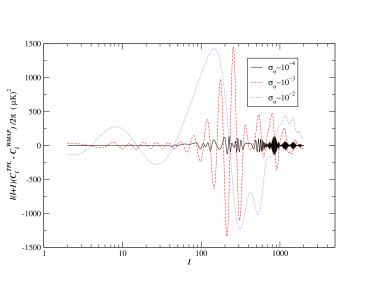
Figure 1: Difference between the trans-Planckian and the standard inflationary multipole moments, plotted for three values of $\sigma_{{}_{0}}$ and for an amplitude of $|x|\sigma_{{}_{0}}=0.3$. A strong damping of the oscillations is observed at large angular scales.

Having checked that the numerical calculations are well under control, one can now move to parameters estimation. The main result of this article is that, with the oscillations taken into account, it is possible to decrease the $\chi^{2}$ significantly. The best fit that has been found by COSMOMC and the result of its Markov chains exploration of the parameter space is summarized in Table 1. It leads to $\chi^{2}\simeq 1415.38$ for $1340$ degrees of freedom, i.e. $\Delta\chi^{2}\simeq 15$ compared to WMAP one. The corresponding multipole moments $C_{\ell}$ and $C_{\ell}^{{\scriptscriptstyle{\mathrm{T}\mathrm{E}}}}$ together with the WMAP data are represented in the bottom panels of Fig. 2. The reason for such an important improvement of the $\chi^{2}$ is clear from these figures: the presence of the oscillations allows a better fit of the cosmic variance outliers at small scales.

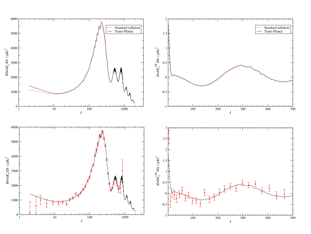
Figure 2: Top left and right panels: the best fit obtained for trans-Planckian angular TT and TE power spectra compared to the best fit standard inflationary power spectra. Bottom left and right panels: the same best fit trans-Planckian TT and TE power spectra but this time compared to the binned WMAP data wmap .

In order to make this statement more quantitative, the difference between the cumulative $\chi^{2}$ with and without the oscillations (in this last case this is nothing but the WMAP cumulative $\chi^{2}$) has been plotted in Fig. 3 as function of the angular scale $\ell$.

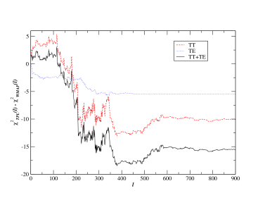
Figure 3: Cumulative residual $\Delta\chi^{2}(\ell)$ between the trans-Planckian fit and the WMAP best fit. The contributions stemming from the temperature and the polarization angular power spectra are also plotted. The final $\Delta\chi^{2}$ improvement is of order $15$.

This permits a direct comparison with the Fig. 4 of Ref. spergel . Clearly, the significant decrease of the $\chi^{2}$ comes from the outliers around the first acoustic peak which are well fitted by the oscillating component of our initial power spectra. Notice also that the outliers at large scales, $\ell<50$, can not be well fitted in this model due to the strong damping described above [see Eq. (13)]. But, as already mentioned several times, this is not a problem since the outliers that contributes the most to the $\chi^{2}$ are not located at large scales but around the first acoustic peak.

To conclude this section, let us remark that we have not given confidence values for the best fit model parameters in Table 1. This is due to the fact that the high-accuracy CAMB version, which is necessary to obtain physical results when the oscillations are included, takes a few minutes to compute only one model instead of a few seconds in the standard inflationary case. Although minima in the $\chi^{2}$ hypersurface can be “rapidly” found with COSMOMC , the Markov chains take a much longer time to scan the “one-sigma” neighborhood. In addition, as studied in Ref. steen , the likelihood function looks like a hedgehog in the parameters space forbidding a smooth convergence of the Markov chains around a given $\chi^{2}$ minimum.

IV Discussion and conclusion

Given the previous result, $\Delta\chi^{2}\simeq 15$, the first question that one may ask is whether the improvement is statistically significant? We have introduced two new parameters, $\sigma_{{}_{0}}$ and $x$, and one may wonder whether it was worth it, given the decrease observed in the $\chi^{2}$. Indeed, it could just be due to statistical fluctuations in the larger parameters space. Since it is not possible to directly compare the $\chi^{2}$ of models with different degrees of freedom, i.e. with different number of parameters, we need another reliable statistical test. The F–test statappl is an efficient tool to deal with this problem. This test works as follows. Given a first fit with $n_{{}_{1}}$ degrees of freedom and with a $\chi^{2}_{{}_{1}}$ and a second fit with $n_{{}_{2}}<n_{{}_{1}}$ degrees of freedom and a new $\chi^{2}_{{}_{2}}<\chi^{2}_{{}_{1}}$, the F–test gives the probability that the decrease in the $\chi^{2}$ is only due to statistical fluctuations and not to the fact that the underlying model is actually a better fit. Generally, one considers that the improvement is significant if this probability is less than a few $\%$. For our case, the F–probability is F${}_{\rm proba}\simeq 0.06\%$.

A possible loophole would be that, since the F–test is only valid for Gaussian statistics, it could not be applied to the case at hand since the multipole moments obey a different statistics. However, since our result comes from relatively small scales, the central limit theorem applies and the statistics should not deviate too much from the Gaussian one. Therefore, we expect the F–test to give a rather fair estimate. Another test has been to check that a spectrum with a different oscillatory pattern, e.g. with a $k$-dependence instead of $\ln k$ in the cosine function, does not provides us with a fit as good as the trans-Planckian one, in the F–test sense and for a same amount of computed models with COSMOMC . This is indeed the case since we have found $\Delta\chi^{2}\simeq 4$ only (with two new parameters) which is not very statistically significant.

Let us now analyze and discuss the result itself in more details. The first remark is that the baryons contribution is standard since we have $\Omega_{\mathrm{b}}h^{2}\simeq 0.025$. It is therefore compatible with Big Bang Nucleosynthesis even if this is slightly less compatible than the value obtained without oscillations but this difference does not seem to be significant. In the same way, the value of $\Omega_{\mathrm{dm}}$ is not significantly modified compared to the standard one. The same is true for the energy scale of inflation, i.e. for $P_{\mathrm{scalar}}$. On the other hand, we see that the value of $\Omega_{\Lambda}$ is particularly high, as the values of $h$ and the optical depth are. However, this still seems to be admissible, in particular with the SNIa measurements. However, the slow-roll parameters differ significantly compared to their standard values peiris ; saminf ; barger and, as a consequence, the spectral index is modified. This is not surprising and should even be expected: since the trans-Planckian parameters seem to be as statistically significant as the slow-roll ones, their inclusion in the best fit search should have an effect on the determination of the slow-roll parameters. The fact that the best fit cosmological parameters with or without oscillations are not exactly the same illustrates the fact that the determination of these cosmological parameters depends on the shape of the primordial power spectra LLMS .

Let us now study the trans-Planckian parameters in more details. First of all, we see that the best fit is such that the preferred scale $M_{\mathrm{c}}$ is almost four orders of magnitude higher than the Hubble scale during inflation. However, this does not provide us with a measure of $M_{\mathrm{c}}$ since the energy scale of inflation cannot be deduced directly from the data. Nevertheless, a constraint on $H$ has been given in Ref. saminf and leads to $M_{\mathrm{c}}/m_{{}_{\mathrm{Pl}}}<0.1$. On the other hand, from Table 1, one obtains that $4\times 10^{4}\sigma_{{}_{0}}^{2}/\sqrt{\epsilon}\simeq 10^{-2}$. This means that the trans-Planckian amplitude, $|x|\sigma_{{}_{0}}=0.29$, is not compatible with the requirement of negligible backreaction effects [see Eq. (11)]. This is certainly a major difficulty not for the presence of oscillations in the multipole moments (since we have proven that this is statistically significant anyway) but rather for the physical interpretation of those oscillations in terms of trans-Planckian physics. At this point, two remarks are in order. First, the previous calculation does not predict what the modifications coming from the inclusion of the backreaction effects are and, in particular, it does not tell that the backreaction effects will modify the power spectra. It just signals when the backreaction effects must be taken into account. Therefore, despite the fact that we are not able to prove it, it could very well be that the backreaction effects do not modify the $k$-dependence of the oscillations (for instance, it could only renormalize the values of the trans-Planckian parameters). Clearly, this is a very difficult technical question since a check of the above speculation would require a calculation at second order in the framework of the relativistic theory of cosmological perturbations with the trans-Planckian effects taken into account. This is beyond the scope of the present article. Secondly, the physical origin of the oscillations could be different. For instance, in Refs. BCLH ; kaloper , initial power spectra with oscillations were also found but with different physical justifications. In the model of Ref. BCLH , the presence of the oscillations is due to non-standard initial conditions in the framework of hybrid inflation, while in Ref. kaloper a sudden transition during inflation is involved. Of course, it remains to be proven that a different model could produce an oscillatory pattern similar to the trans-Planckian one but since, on a purely phenomenological level, it seems that the significant increase of the likelihood requires superimposed oscillation in the initial power spectra, this is a question that is certainly worth studying. Let us also signal that a primordial bouncing phase, as described for instance in Ref. MP , may also do the job. Finally, let us remind that the main goal of the paper was to study whether the idea that oscillations are present in the WMAP data can be statistically demonstrated and that the trans-Planckian power spectra used before were just one possible example.

As a conclusion, a word of caution is in order. From the previous considerations, it is clear that, in the absence of outliers around the first acoustic peak, there would be no reason, in the F–test sense, to include oscillations with a large amplitude (i.e. $|x|\neq 1$) in the power spectra. Therefore, the future WMAP data release will be extremely important to check whether the presence of these outliers is confirmed or if they are just observational artifacts. However, if the last possibility turns out to be true, it is clear that it would still be worth looking for small trans-Planckian effects (i.e. $|x|=1$) in the future very high-accuracy Planck data and the ideas put forward in the present article would still be useful for this purpose.

- (1) C. L. Bennet et al. , Astrophys. J. Suppl. 148, 1 (2003), eprint astro-ph/0302207.
- (2) G. Hinshaw et al. , Astrophys. J. Suppl. 148, 135 (2003), eprint astro-ph/0302217.
- (3) L. Verde et al. , Astrophys. J. Suppl. 148, 195 (2003), eprint astro-ph/0302218.
- (4) H. V. Peiris et al. Astrophys. J. Suppl. 148, 213 (2003), eprint astro-ph/0302225.
- (5) S. Leach and A. Liddle, Phys. Rev. D68, 123508 (2003), eprint astro-ph/0306305.
- (6) G. Efstathiou, Mon. Not. Roy. Astron. Soc. 343, L95 (2003), eprint astro-ph/0303127.
- (7) C. Contaldi, M. Peloso, L. Kofman and A. Linde, JCAP 0307, 005 (2003), eprint astro-ph/0303636.
- (8) J. M. Cline, P. Crotty and J. Lesgourgues, JCAP 0309, 010 (2003), eprint astro-ph/0304558.
- (9) B. Feng and X. Zhang, Phys. Lett. B570, 145 (2003), eprint astro-ph/0305020; B. Feng, M. Li, R.-J. Zhand and X. Zhang, Phys. Rev. D68, 103511 (2003), eprint astro-ph/0302479.
- (10) S. Tsujikawa, R. Maartens and R. H. Brandenberger, Phys. Lett. B574, 141 (2003), eprint astro-ph/0308169.
- (11) J.-P. Luminet et al. , Nature 425, 593 (2003).
- (12) Q.-G. Huang and M. Li, JCAP 0311, 001 (2003), eprint astro-ph/0308458; JHEP 06, 014 (2003), eprint hep-th/0304203.
- (13) G. Efstathiou, Mon. Not. Roy. Astron. Soc. 346, L26 (2003), eprint astro-ph/0306431; 348, 885 (2004), eprint astro-ph/0310207.
- (14) D. N. Spergel et al. , Astrophys. J. Suppl. 148, 175 (2003), eprint astro-ph/0302209.
- (15) X. Wang, B. Feng and M. Li, eprint astro-ph/0209242.
- (16) J. Martin and R. H. Brandenberger, Phys. Rev. D63, 123501 (2001), eprint hep-th/0005209.
- (17) R. H. Brandenberger and J. Martin, Mod. Phys. Lett. A16, 999 (2001), eprint astro-ph/0005432.
- (18) J. C. Niemeyer, Phys. Rev. D63, 123502 (2001), eprint astro-ph/0005533.
- (19) M. Lemoine, M. Lubo, J. Martin and J. P. Uzan, Phys. Rev. D65, 023510 (2002), eprint hep-th/0109128.
- (20) A. Kempf, Phys. Rev. D63, 083514 (2001), eprint astro-ph/0009209.
- (21) R. Easther, B. R. Greene, W. H. Kinney and G. Shiu, Phys. Rev. D64, 103502 (2001), eprint hep-th/0104102.
- (22) R. Easther, B. R. Greene, W. H. Kinney and G. Shiu, Phys. Rev. D67, 063508 (2003), eprint hep-th/0110226.
- (23) A. Kempf and J. C. Niemeyer, Phys. Rev. D64, 103501 (2001), eprint astro-ph/0103225.
- (24) R. H. Brandenberger and P. M. Ho, Phys. Rev. D66, 023517 (2002), eprint hep-th/0203119.
- (25) S. F. Hassan and M. S. Sloth, Nucl. Phys. B674, 434 (2003), eprint hep-th/0204110.
- (26) F. Lizzi, G. Mangano, G. Miele and M. Peloso, JHEP 0206, 049 (2002), eprint hep-th/0203099.
- (27) U. H. Danielsson, Phys. Rev. D66, 023511 (2002), eprint hep-th/0203198.
- (28) R. Easther, B. R. Greene, W. H. Kinney and G. Shiu, Phys. Rev. D66, 023518 (2002), eprint hep-th/0204129.
- (29) G. L. Alberghi, R. Casadio and A. Tronconi, Phys. Lett. B579, 1 (2004), eprint gr-qc/0303035.
- (30) C. Armendáriz-Picón and E. A. Lim, JCAP 12, 006 (2003), eprint hep-th/0303103.
- (31) J. Martin and R. H. Brandenberger, Phys. Rev. D68, 063513 (2003), eprint hep-th/0305161.
- (32) J. Martin and D. J. Schwarz, Phys. Rev. D67, 083512 (2003), eprint astro-ph/0210090.
- (33) V. F. Mukhanov, H. A. Feldman and R. H. Brandenberger, Phys. Rept. 215, 203 (1992).
- (34) J. Martin and D. J. Schwarz, Phys. Rev. D57, 3302 (1997), eprint astro-ph/9704049.
- (35) E. D. Stewart and D. H. Lyth, Phys. Lett. B302, 171 (1993).
- (36) D. J. H. Chung, A. Notari and A. Riotto, JCAP 0310, 012 (2003), eprint hep-ph/0305074.
- (37) T. Banks and L. Mannelli, Phys. Rev. D67, 065009 (2003), eprint hep-th/0209113.
- (38) M. B. Einhorn and F. Larsen, Phys. Rev. D67, 024001 (2003), eprint hep-th/0209159.
- (39) N. Kaloper et al. , JHEP 0211, 037 (2002), eprint hep-th/0209231.
- (40) K. Goldstein and D. A. Lowe, Nucl. Phys. B669, 325 (2003), eprint hep-th/0302050.
- (41) H. Collins, R. Holman and M. R. Martin, Phys. Rev. D68, 124012 (2003), eprint hep-th/0306028.
- (42) H. Collins and R. Holman, eprint hep-th/0312143.
- (43) J. Martin and D. J. Schwarz, Phys. Rev. D62, 103520 (2000), eprint gr-qc/9704049.
- (44) J. Martin, A. Riazuelo and D. J. Schwarz, Astrophys. J. 543, L99 (2000), eprint astro-ph/0006392.
- (45) L. Bergstrom and U. H. Danielsson, JHEP 0212 038 (2002), eprint hep-th/0211006.
- (46) Ø. Elgarøy and S. Hannestad, Phys. Rev. D68, 123513 (2003), eprint astro-ph/0307011.
- (47) A. Kogut et al. , Astrophys. J. Suppl. 148, 161 (2003), eprint astro-ph/0302213.
- (48) L. Hui and W. Kinney, Phys. Rev. D65, 103507 (2002), eprint astro-ph/0109107.
- (49) A. Lewis, A. Challinor and A. Lasenby, Astrophys. J. 538, 473 (2000), eprint astro-ph/9911177, http://camb.info.
- (50) S. Leach, http://astronomy.sussex.ac.uk/~sleach/inflation/camb_inflation.html.
- (51) A. Lewis and S. Bridle, Phys. Rev. D66, 103511 (2002), eprint astro-ph/0205436, http://cosmologist.info/cosmomc.
- (52) V. Barger, H.-S. Lee and D. Marfatia, Phys. Lett. B565, 33 (2003), eprint hep-ph/0302150.
- (53) W. Hu and T. Okamoto, Phys. Rev. D69, 043004 (2004), eprint astro-ph/0308049.
- (54) D. J. Schwarz, C. A. Terrero-Escalante and A. A. Garcia, Phys. Lett. B517, 243 (2001), eprint astro-ph/0106020.
- (55) I. S. Gradshteyn and I. M. Ryzhik, Tables of Integrals, Series and Products, Academic, New York, 1981.
- (56) CETAMA (Commission d’établissement des méthodes d’analyses du commissariat à l’énergie atomique), Statistique appliquée à l’exploitation des mesures”, Masson, Paris, 1986.
- (57) S. Leach, A. R. Liddle, J. Martin and D. J. Schwarz, Phys. Rev. 66, 023515 (2002), eprint astro-ph/0202094.
- (58) C. P. Burgess, J. M. Cline, F. Lemieux and R. Holman, JHEP 0302, 048 (2003), eprint hep-th/0210233.
- (59) N. Kaloper and M. Kaplinghat, Phys. Rev. D68, 123522 (2003), eprint hep-th/0307016.
- (60) J. Martin and P. Peter, Phys. Rev. D68, 103517 (2003), eprint hep-th/0307077.