Characterising stellar micro-variability for planetary transit searches

A method for simulating light curves containing stellar micro-variability for a range of spectral types and ages is presented. It is based on parameter-by-parameter scaling of a multi-component fit to the solar irradiance power spectrum (based on VIRGO/PMO6 data), and scaling laws derived from ground based observations of various stellar samples.

A correlation is observed in the Sun between the amplitude of the power spectrum on long (weeks) timescales and the BBSO Ca ii K-line index of chromospheric activity. On the basis of this evidence, the chromospheric activity level, predicted from rotation period and $B-V$ colour estimates according to the relationship first introduced by Noyes (1983) and Noyes et al. (1984), is used to predict the variability power on weeks time scale. The rotation period is estimated on the basis of a fit to the distribution of rotation period versus $B-V$ observed in the Hyades and the Skumanich (1972) spin-down law. The characteristic timescale of the variability is also scaled according to the rotation period.

This model is used to estimate the impact of the target star spectral type and age on the detection capability of space based transit searches such as Eddington and Kepler. K stars are found to be the most promising targets, while the performance drops significantly for stars earlier than G and younger than 2.0 Gyr. Simulations also show that Eddington should detect terrestrial planets orbiting solar-age stars in most of the habitable zone for G2 types and all of it for K0 and K5 types.

1 Introduction

The transit method is reaching maturity as a method to discover gaseous giant exo-planets from the ground. Several transit-search projects have now produced convincing candidates, which are awaiting confirmation through other methods.

However, the few years of experience now available in this field have exemplified the difficulty of the task at hand. The signal is small ($\approx 2$ % at most), short (a few hours), with periods ranging from a few days to several years, and is embedded in noisy data (photon, sky, background, instrumental noise, etc…). Ground-based projects also suffer from the daily interruptions in the observations and the finite duration of the observing runs, and are affected by atmospheric scintillation noise. A variety of transit search algorithms have been developed, ranging from a simple matched filter to more sophisticated methods (Doyle et al., 2000; Defaÿ et al., 2001; Aigrain & Favata, 2002; Kovács et al., 2002). All of these are optimised to work in the presence of white noise, and tests of simulated data have shown they can perform very well, reliably detecting transits at the extreme margin of statistical significance. Rather than the detection of the transits themselves, the major difficulty for ground-based searches has in fact been distinguishing transit-like events caused by stellar systems, such as eclipsing binaries with high mass ratios, or hierarchical triple systems (due to either a physical triple system or and eclipsing binary blended with a foreground star), from true planetary transits.

In order to detect terrestrial planets, it is necessary to go to space, to avoid being affected by atmospheric scintillation and to monitor the target field(s) continuously, with minimal interruptions. However, with improved photometric precision comes an additional noise source, which is usually insignificant at the precisions achieved by ground based observations: the intrinsic variability of the stars, due mainly to the temporal evolution and rotational modulation of structures on the stellar disk. The Sun’s total irradiance (see Fig. 1) varies on all timescales covered by the available data, with a complex, non white power spectrum (see Fig. 2). The amplitude of the variations can reach more than $1$ % when a large spot crosses the solar disk at activity maximum, compared to transit depths of tenths to hundredths of a percent. There is significant power on timescales of a few hours, similar to the typical transit duration. Thus Sun-like variability, if left untreated, would significantly affect the detection performance of missions such as Eddington or Kepler (Aigrain et al., 2001).

Eddington (Favata, 2003) is an ESA mission to be implemented as part of the Agency’s  “Cosmic Vision” science program, with a planned launch date in 2007/2008. Its two primary goals are the study of stellar structure and evolution through asteroseismology, and the detection of habitable planets via the transit method. Kepler (Borucki et al., 2003) is a NASA Discovery mission which will concentrate primarily on the second of these two goals, and is planned for launch in 2008.

A number of algorithms designed to reduce the impact of micro-variability have been tested on simulated data (Defaÿ et al., 2001; Jenkins, 2002; Carpano et al., 2003). Some are modified detection algorithms, designed to differentiate between the transit signal and the stellar noise. Others are pre-processing tools, which whiten the noise profile before running standard transit detection algorithms. Inserting solar irradiance data from VIRGO into simulated light curves, Carpano et al. (2003) showed that the transit detection performance achieved in the presence of Sun-like variability after pre-processing can be as good as that obtained with unprocessed light curves containing white noise only. Jenkins (2002) applied a simple scaling to the solar irradiance data to evaluate the impact of increased rotation rate. Nonetheless, a more physical model, in which the different phenomena involved can be scaled independently in timescale and amplitude for a range of spectral types and ages, is needed to simulate realistic light curves for stars other than the Sun. This will allow us to optimise, evaluate and compare different algorithms, but also different design and target field options for the space missions concerned.

The present paper is concerned with the development of such a model. The philosophy adopted in the process is the following. Intrinsic stellar variability is by no means a well-understood process. Despite recent progress in the modelling of activity-induced irradiance variations on timescales of days to weeks in the Sun (Krivova et al., 2003; Lanza et al., 2003), the extension of these physical models to other stars remains problematic, due to the scarcity of information on how the timescales, filling factors of various surface structures, and contrast ratios, depend on stellar parameters. We have therefore adopted an empirical approach, using chromospheric flux measurements as a proxy measure of activity-induced variability. This step is possible due to the fact that a correlation between the two quantities is observed in the Sun throughout its activity cycle, as well as in other stars. Similarly, empirically derived relationships were used again to relate chromospheric activity, rotation, age and colour, rather than attempting to use models which make a number of assumptions about the physical process driving these phenomena, and generally depend on parameters which require fine-tuning.

The analysis of the evolution of the Sun’s total irradiance variations with the solar activity cycle is described in Sect. 2: the power spectrum of the variations is modelled as a sum of powerlaws, whose parameters are tracked as they evolve throughout the solar cycle. The same type of model is used to construct artificial power spectra and light curves for stars with given theoretical parameters (age, spectral type). A number of empirically derived scaling laws are used to relate these input stellar parameters to the power spectrum parameters (Sect. 3). As a consistency check and an illustration of the possible applications of this model, the results of a small set of simulations designed to evaluate the impact of variability from different stars on Eddington’s planet-hunting capabilities are described in Sect. 4.

2 Clues from solar irradiance variations

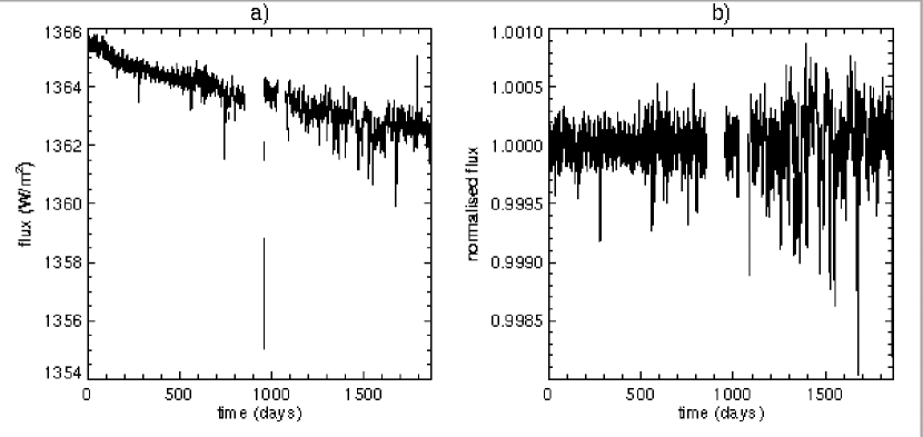
Figure 1: PMO6 light curve, a) before and b) after the pre-processing steps described in Sect. 2.1.1. The data starts in January 1996.

The Sun is the only star observed with sufficient precision and frequent sampling to permit detailed micro-variability studies, thanks to the recent wealth of data collected by the SoHO spacecraft, and particularly the full disk observations obtained by VIRGO (Variability of solar IRradiance and Gravity Oscillations), the experiment for helioseismology and solar irradiance monitoring on SoHO, (Frohlich et al., 1997).

Stellar micro-variability is difficult to observe from the ground due to its very low amplitude, except for very young, active stars – which are outside the main range of interest for planet searches. There is some information available on rms night-to-night and year-to-year photometric variability of a small sample of stars monitored over many years by a few teams (Radick et al., 1998; Henry et al., 2000). We make use of these as they present the advantage of covering a range of stellar ages, but their irregular time coverage and limited photometric precision make them unsuitable for an in-depth study, and particularly for the detailed analysis of the frequency content of the variations.

A drastic improvement in our understanding of intrinsic stellar variability across the HR diagram is expected from the very missions this work is aimed at preparing. In the relatively short term, MOST will provide valuable information for a small sample of stars, but it is not until the launch of COROT, and later Kepler and Eddington, that a wide range of stellar parameters will be covered. In the mean time, we must make use of the detailed solar data, and make reasonable assumptions to extrapolate to other stars than the Sun.

2.1 SoHO/VIRGO total irradiance (PMO6) data

All SoHO/VIRGO data used in this work were kindly provided by the VIRGO team. The main instrument of interest was PMO6, a radiometer measuring total solar irradiance.

The light-curves cover the period January 1996 to March 2001, which roughly corresponds to the rising phase of cycle 23.

2.1.1 Pre-processing of the data

The light curves were received as level 1 data, in physical units but with no correction for instrumental effects or outliers. Careful treatment was required to remove long term (instrument decay) trends. There was a difference of $\sim 0.24$ % in the mean measured flux between the start and the end of the time series. Given that the observations roughly correspond to the interval between the minimum and the maximum of the Sun’s activity cycle, one might expect to see a rise in the mean irradiance over that period. The instrumental decay may therefore be higher than the value quoted. However, the absolute value of the irradiance was of little interest for the present study, which concentrates on relative variations on time scales of weeks or less. Any long term trends in the data were therefore removed completely, regardless of whether they were of instrumental or physical origin. The decay appeared non-linear and there were discontinuities and outliers in the light curves, making a simple spline fit unsuitable.

The approach that was adopted consisted of a 3 step process:

• Obvious outliers were removed by computing residuals from a spline fit (whose nodes were spaced two months apart to avoid being sensitive to the Sun’s rotation period) and applying a 1 $\sigma$ cutoff.

• Visual inspection of the data then allowed us to manually remove sections visibly affected by instrumental problems.

• Spline fits were performed on intervals chosen by visual inspection to start and end where discontinuities occurred. Each interval was divided by the corresponding fit, resulting in a normalised output light curve.

• A 5 $\sigma$ cutoff was applied for outlier removal.

• The sampling, originally 1 min, was reduced to 15 min to make the size of the light curves more manageable. This was done by taking the mean of the original data points in each 15 min bin, ignoring any missing or bad data points. It is unlikely any information on timescales shorter than 15 min would significantly impact the transit detection process, as the transits of interest here generally last several hours (corresponding to orbital periods of several months or years).

• Data gaps were replaced with the baseline value of $1.0$, to allow the calculation of the power spectra needed for the analysis.

2.2 Modelling the ‘solar background’

The power spectrum of the solar irradiance variations at frequencies lower than $\simeq 8$ mHz constitutes a noise source for helioseismology, usually referred to as the ‘solar background’. It is common practice to fit this background with a sum of powerlaws in order to model it accurately enough to allow the measurement of solar oscillation frequencies and amplitudes. Powerlaw models were first introduced by Harvey (1985). The most commonly used model in the literature today is that of Andersen et al. (1994), which is fairly similar: the total power spectrum is approximated by a sum of power laws, the number $N$ of which varies between three and five depending on the frequency coverage:

$$P(\nu)=\displaystyle{\sum_{i=1}^{N}}P_{i}=\displaystyle{\sum_{i=1}^{N}}\frac{A_{i}}{1+(B_{i}\leavevmode\nobreak\ \nu)^{C_{i}}}$$ (1)

where $\nu$ is frequency, $A_{i}$ is the amplitude of the $i^{\mathrm{th}}$ component, $B_{i}$ is its characteristic timescale, and $C_{i}$ is the slope of the power law (which was fixed to $2$ in Harvey’s early model). For a given component, the power remains approximately constant on timescales larger than $B$, and drops off for shorter timescales. Each power law corresponds to a separate class of physical phenomena, occurring on a different characteristic time scale, and corresponding to different physical structures on the surface of the Sun (see Table 1).

Table 1: Typical timescales for the different of structures on the solar surface.

$$\begin{array}[]{p{0.5\linewidth}l}\hline\cr\vskip 3.0pt plus 1.0pt minus 1.0pt\cr Component&\mathrm{Timescale}\leavevmode\nobreak\ B\leavevmode\nobreak\ (\mathrm{s})\\ \vskip 3.0pt plus 1.0pt minus 1.0pt\cr\hline\cr\vskip 3.0pt plus 1.0pt minus 1.0pt\cr Active\leavevmode\nobreak\ regions&1\leavevmode\nobreak\ \mathrm{to}\leavevmode\nobreak\ 3\times 10^{7}\\ Super-granulation&3\leavevmode\nobreak\ \mathrm{to}\leavevmode\nobreak\ 7\times 10^{4}\\ Meso-granulation&\simeq 8000\\ Granulation&200\leavevmode\nobreak\ \mathrm{to}\leavevmode\nobreak\ 500\\ Bright\leavevmode\nobreak\ points&\simeq 70\\ \vskip 3.0pt plus 1.0pt minus 1.0pt\cr\hline\cr\end{array}$$

2.3 Evolution of the power spectrum with the activity cycle

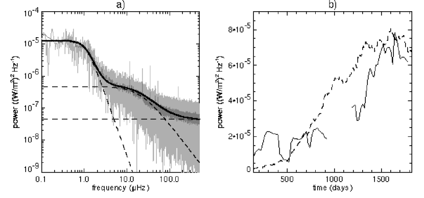
Figure 2: a) Power spectrum of the PMO6 light curve (1996-2001). Light grey: power spectrum. Dark grey: idem, smoothed with a boxcar algorithm. Thick solid line: multi-component powerlaw fit (see Sect. 2.2). Dotted lines: individual components of the fit. b) Comparison between the the time dependence of the amplitude of the low frequency component of the power spectrum ($A_{1}$) and chromospheric activity. Solid line: Evolution of $A_{1}$, computed as described in Sect. 2.3, using $L=180$ days and $S=20$ days, between 1996 and 2001. The gap at around 1000 days corresponds to a prolonged gap in the data. Dotted line: BBSO Ca ii K-line index over the same period (arbitrary units), smoothed with a boxcar algorithm (base $180$ days).

In order to track the evolution of the solar background over the activity cycle, sums of power-laws – as given by Eq. 1 – were fitted to the power spectrum of a section of data of duration $L$ (typically 6 months). Such a fit is illustrated on the power spectrum of the entire dataset in the left-hand panel of Fig. 2. The operation is then repeated for a section shifted by a small interval $S$ from the previous one (typically 20 days), and so on. Thus the evolution of each component can be tracked throughout the rise from solar minimum (1996) to maximum (2001) by measuring changes in the parameters defining each powerlaw.

A single component fit with parameters $A_{1}$, $B_{1}$ & $C_{1}$ is made first. Additional components are then added until they no longer improve the fit, i.e. until the addition of an extra component does not reduce the $\chi^{2}$ by more than $10^{-2}$. The fit to the first section is used as the initial guess for the fit to the next section, and so forth. This method allows us to track the emergence of components corresponding to different types of surface structures throughout the solar cycle, as well as monitor variations in amplitude, timescale and slope for each component.

Figure 3: Scatter plot of the amplitude of the low frequency component of solar irradiance variations $A_{1}$ (computed as described in Sect. 2.3, using $L=180$ days and $S=20$ days), versus the BBSO Ca ii K-line index (arbitrary units) over the period 1996 to 2001.

2.3.1 Results

The algorithm described above was run on the PMO6 data with $L=180$ days and $S=20$ days, and three components were found to provide the best fit in all cases. These components have stable timescales and slope, varying in amplitude only. The physical processes giving rise to each component are thus of a permanent nature. A number of points of interest emerge from the results. The first component, with $\tau\simeq 1.3\times 10^{5}$ s (active regions) shows an increasing trend in amplitude which is well correlated with the Ca ii K-line index, an indicator of chromospheric activity. This is illustrated in the right-hand panel of Fig. 2. The slope of the powerlaw is 3.8 (in good agreement with Andersen et al., 1998).

The observed correlation, which is further illustrated by the scatter plot in Fig. 3 comes as no surprise. The passage of individual active regions across the disks of the Sun and other stars monitored by the Mt Wilson HK Project can be clearly seen in plots of the activity index $S$ (from which $R^{\prime}_{\mathrm{HK}}$ is derived) versus time. On the other hand, the effect of the same type of event on the solar irradiance has been studied with a number of instruments, most recently VIRGO/LOI and PMO6 (Domingo et al., 1998). Recent models including contributions from faculae and sunspots of tunable size and number reproduce the PMO6 light curve to a high degree of precision (Krivova et al., 2003; Lanza et al., 2003).

However, observing and characterising a correlation throughout the Sun’s activity cycle, between a chromospheric activity indicator which can be measured from the ground for a large number of stars, and total irradiance variations, whose amplitudes are so small they are only observable by dedicated high-precision photometric space missions, goes one step further. Most importantly for planetary transit searches, it implies that chromospheric activity indicators such as $R^{\prime}_{\mathrm{HK}}$ can be used as a proxy to predict weeks timescale variability levels for a wide range of stars.

The amplitude of the second component also increases, but is not correlated to the Ca ii index. This component corresponds to timescales corresponding to super- and meso- granulation, for which no detailed models are available to date. Our understanding of this kind of phenomenon is expected to improve dramatically when the results from space-based experiments designed for precision time-series photometry will become available.

2.3.2 Implications

The correlation between $A_{1}$ and the Ca ii K-line index, although not extremely tight, is a clear indication that chromospheric activity indicators contain information about the variability level of the Sun on timescales longer than a few days. To establish more solidly a scaling law between photometric variability and chromospheric activity, we must use a wider stellar sample to constrain the relation over the entire expected range of activity levels (see Sect. 3.3).

Little useful information has been extracted from the solar data on what determines the parameters of the solar background other than $A_{1}$. The few clues available from other sources will be presented in Sect. 3.4.

3 Modelling stellar micro-variability

The main aim of the present model is the simulation of realistic light curves of stars more active than the Sun, if possible as a function of stellar parameters such as spectral type and age, via observables such as $B-V$ colour and rotational period $P_{\mathrm{rot}}$. The multi-component power-law model used in Sect. 2 to fit the solar background power spectrum now forms the basis of the simulation of enhanced variability light curves.

To simulate a light curve for a given star, the first task is to generate a power spectrum using this power-law model. When applying the component-by-component procedure described in Sect. 2.3 to fit solar power spectra, the optimal number of components was found to be three. We therefore use a sum of three power-laws to generate the stellar power spectra. The highest frequency component, a superposition of granulation, oscillations and white noise, has a characteristic timescale which is shorter than the typical sampling time for planetary transit searches, and thus can be replaced by a constant value. There are therefore a total of 7 parameters to adjust for each simulated power spectrum: three for each resolved power-law plus one constant.

The inputs of the model are the spectral type and age of the star. Starting from these theoretical quantities given, how are the power-law parameters deduced? Most of the information available concerns the amplitude of the first power-law, $A_{1}$. We have established in Sect. 2 that there is a correlation between $A_{1}$ and the Ca II K-line indicator of chromospheric activity. On the other hand, there is a well known scaling between rotation period, colour and chromospheric activity (Noyes et al., 1984). Provided one can estimate the rotation period of the star (see Sect. 3.1), the activity level is computed (Sect. 3.2), and from this one obtains $A_{1}$ (Sect. 3.3). Sect. 3.4 summarises how the other parameters of the power-law model, on which much less information is available, are estimated.

3.1 The rotation period-colour-age relation

As detailed in Sect. 3.2, it is possible to deduce the expected activity level for a star of known mass (i.e. colour) and rotation period. However, the number of stars with known rotation periods is relatively small. In the context of the present work, it would thus be useful to be able to predict the rotation period for a given stellar mass and age.

Observational constraints on rotation rates for stars of known mass and age come from two sources: star forming regions and young open clusters, where one can measure photometric rotation periods or rotational line broadening ($v\sin i$); and the Sun itself. There is little else, as rotational measurements are hard to perform for all the quiet, slowly rotating intermediate age and old stars other than the Sun, except for relatively nearby field stars, for which little reliable age information is available. The status of observational evidence and theoretical modelling in this domain is outlined by Krishnamurthi et al. (1997), Bouvier et al. (1997) and Stassun & Terndrup (2003). Here we briefly sketch the current paradigm to set the context of the present work.

The observed initial spread in rotation velocities (from measurements of T-Tauri stars, with a concentration around $10$–$30$ km s^-1 but a number of fast rotators, up to $100$’s of km s^-1) is attributed to the competing effects of spin-up (due to the star’s contraction and accretion of angular momentum from the disk) and slowing-down mechanisms such as disk-locking (Königl, 1991; Bouvier et al., 1997). This spread is observed to diminish with age (by the age of the Hyades, only some M-dwarfs still exhibit fast rotation, Prosser et al. 1995), leading to a dependency of rotation on mass only. Following this homogenisation, one observes constant spin-down in a given mass range (cf. the Skumanich 1972 $t^{1/2}$ law for Sun-like stars). Both homogeneisation and power-law spin-down can be explained by the loss of angular momentum through a magnetised wind (Schatzman, 1962; Weber & Davis, 1967), a mechanism which is more effective in faster rotators.

Angular momentum evolution models have vastly improved recently, but they still rely on the careful tuning of a number of parameters, especially for young and low-mass stars. We have therefore chosen to use empirically derived scaling laws and to restrict ourselves to the range of ages (older than the Hyades) and spectral types (mid-F to mid-K) where a unique colour-age-rotation relation can be established. In this range the forementioned parameters become less relevant and the models reproduce the observations fairly robustly.

A relationship between $B-V$ colour (i.e. mass) and rotation at a given age was empirically derived from photometric rotation period measurements in the Hyades (Radick et al., 1987, 1995). Only rotation periods were used, rather than $v\sin i$ measurements, to avoid introducing the extra uncertainty of assigning random inclinations to the stars and having to assume theoretical radii to convert $v\sin i$ to a period. This relationship is valid for the range $0.45\leq B-V\leq 1.3$. For stars bluer than $B-V=0.45$, rotation rates saturate, but this is outside the range of spectral types of interest for the present work. Redder than $B-V=1.3$, a significant spread is still observed in the rotation periods. The remaining range is divided into two zones, each following a linear trend. Redder than $B-V=0.62$, the slope of the relation is quite close to the theoretical relation obtained by Kawaler (1989). We also estimated the age of the Hyades from the zero-point of the linear fit as done by Kawaler (1989), but incorporating the improved data from Radick et al. (1995). The age obtained in this manner is $634$ Myr, consistent with recent determinations by independent methods: $655$ Myr (Cayrel de Strobel, 1990), $600$ Myr (Torres et al., 1997), and $625$ Myr (Perryman et al., 1998), thereby confirming the quality of the fit. The slope for stars bluer than $B-V=0.62$ is much steeper, presumably due to the thinner convective envelopes of the stars in this range.

Figure 4: Plot of rotation period versus $B-V$ colour for Hyades stars. Data from Radick et al. (1987, 1995). The thin parallel black lines correspond to ‘rotational isochrones’ from Kawaler (1989) with $t$ as indicated next to each line (in units of $10^{8}$ yr). The dashed line is a linear fit to the data with $0.6\leq B-V<1.3$. The thick solid line is a composite of two linear fits, one for $B-V<0.62$ and one for $0.62\leq B-V<1.3$.

This can then be combined with the $t^{1/2}$ spin-down law into a rotation-colour-age relation:

$$\begin{array}[]{l}\log\left(P_{\mathrm{rot}}\right)-0.5\leavevmode\nobreak\ \log\left(\frac{t}{625\leavevmode\nobreak\ \mathrm{Myr}}\right)=\vspace{0.3cm}\\ \hskip 14.22636pt\left\{\begin{array}[]{rr}-0.669+2.580\leavevmode\nobreak\ (B-V),&0.45\leq B-V<0.62\\ 0.725+0.326\leavevmode\nobreak\ (B-V),&0.62\leq B-V<1.30\end{array}\right\}\end{array}$$ (2)

A comment on the adopted value of $0.5$ for $n_{t}$, the index in the spin-down law is appropriate. It has recently been suggested that a $0.6$ might be more appropriate (Guinan & Ribas 2002, on the basis of an updated sample of Sun-like stars with some new age determinations). However, the original value of $0.5$ was kept for the present work. The change would not affect the predicted rotation rates significantly, and the errors on this new value of $n_{t}$ (which depends, for example, on age determinations from isochrone fitting) are larger than the difference. We have therefore kept the lower value, as it leads, if in error, to overestimated rotation rates, hence more variability and on faster timescales, and eventually conservative estimates of transit detection rates.

3.2 The activity-rotation period-colour relation

The next step consists in estimating from the colour and rotation period the expected chromospheric activity level of the star. For this purpose, the scaling law first derived by Noyes (1983) and Noyes et al. (1984) is used. It relates the Ca ii index $\left<R^{\prime}_{\mathrm{HK}}\right>$ to the inverse of the Rossby number $R_{\mathrm{o}}$, and can thus be understood in terms of the interplay between convection, rotation and the star’s dynamo:

$$-\log R_{\mathrm{o}}=0.324-0.400\leavevmode\nobreak\ y+0.283\leavevmode\nobreak\ y^{2}-1.325\leavevmode\nobreak\ y^{3}$$ (3)

where $y=\log\left<R^{\prime}_{\mathrm{HK}}\right>_{5}$ and $\left<R^{\prime}_{\mathrm{HK}}\right>_{5}=\left<R^{\prime}_{\mathrm{HK}}\right>\times 10^{5}$. $R_{\mathrm{o}}$ is related to the rotation period $P_{\mathrm{rot}}$ and $B-V$ colour as follows:

$$R_{\mathrm{o}}=\tau_{\mathrm{c}}/P_{\mathrm{rot}}$$ (4)

where $P_{\mathrm{rot}}$ is expressed in days, and the following (empirically derived) relation for $\tau_{\mathrm{c}}$, the convective overturn time, is used:

$$\begin{array}[]{l}\log\left(\tau_{\mathrm{c}}\right)=\vspace{0.3cm}\\ \hskip 14.22636pt\left\{\begin{array}[]{lcl}1.361-0.166\leavevmode\nobreak\ x+0.025\leavevmode\nobreak\ x^{2}-5.323\leavevmode\nobreak\ x^{3},&&x\geq 0\\ 1.361-0.140\leavevmode\nobreak\ x,&&x<0\end{array}\right\}\end{array}$$ (5)

where $x=1-(B-V)$. Equation (3) was inverted (using an interpolation between tabulated values) to allow us to deduce the chromospheric activity index from the rotation period and $B-V$ colour of a star. For details of how the above relations, which are simply stated here, were obtained, the reader is referred to Noyes et al. (1984).

3.3 Active regions variability and chromospheric activity

Having noted that the ‘active regions’ component of the solar activity spectrum appears directly correlated to chromospheric activity (see Sect. 2.3), we turn to the small but valuable datasets containing both photometric variability measurements and activity indexes for a variety of stars. The data available on any one star is of course much less precise and less reliable than the solar data, but the dataset as a whole spans a much wider range of activity levels.

We use a sample of stars for which both $\left<R^{\prime}_{\mathrm{HK}}\right>$ and rms photometric variability measurements are available in the litterature. This sample, mainly taken from Radick et al. (1998) and Henry et al. (2000), covers a wide range of spectral types and ages, including the active young (130 Myr) solar analogue EK Dra and some older, Sun-like stars which are known to harbour planets from radial velocity measurements.

These data can be used to derive a quantitative relationship between $\left<R^{\prime}_{\mathrm{HK}}\right>$ and night-to-night rms variability (in Strömgren $b$ and $y$; $\mathrm{rms}_{by}=\mathrm{rms}\{(b+y)/2\}$). All rms values used are in units of $10^{-4}$ mag.

Figure 5: Plot of $\mathrm{rms}_{by}$ versus $\left<R^{\prime}_{\mathrm{HK}}\right>_{5}$ for a sample of stars from Radick et al. (1998) and Henry et al. (2000), with $2^{\mathrm{nd}}$ order polynomial fit overlaid.

As illustrated in Fig. 5, a $2^{\mathrm{nd}}$ order polynomial provides a good fit to the relationship between $\mathrm{rms}_{by}$ and $\left<R^{\prime}_{\mathrm{HK}}\right>_{5}$. The equation of the fit is:

$$\mathrm{rms}_{by}=3.69+4.60\leavevmode\nobreak\ \left<R^{\prime}_{\mathrm{HK}}\right>_{5}+2.88\leavevmode\nobreak\ \left<R^{\prime}_{\mathrm{HK}}\right>_{5}^{2}$$ (6)

Note that one star, EK Dra, is significantly more active and variable than the rest of the sample – because it is younger. Including it in the fit thus gives it a disproportionate weight, but we have included it because it broadens the range of $\left<R^{\prime}_{\mathrm{HK}}\right>$ covered by a factor of 2. Furthermore, previous studies have shown (Messina & Guinan, 2002) that it fits tightly on relationships between activity and stellar parameters derived from samples of solar analogues of various ages, suggesting its behaviour is representative of the mechanisms driving activity in general – and thus, in our reasoning, variability on the timescales under consideration.

To be usable for our purposes, Eq. (6) must be completed by relationship between $\mathrm{rms}_{by}$ and $A_{1}$. The desired value of $A_{1}$ corresponds to white light relative flux variations, not $b$ and $y$ magnitude variations. To obtain the rms of the relative flux variations one must multiply the rms of the magnitude variations by a constant factor of $2.5/\ln(10)=1.08$. This must then be converted to a white light flux rms value. This requires the definition of a reference point in the solar cycle, at which to compare the variability levels in the two bandpasses. Radick et al. (1998) quote a single $\log\left<R^{\prime}_{\mathrm{HK}}\right>$ value of $-4.89$ for the Sun, which is an average of measurements performed over many years. This defines a reference solar activity level, corresponding roughly to a third of the way into the rising phase of cycle 23. The average night-to-night variability as measured in $b$ and $y$ by Radick et al. (1998) is $\mathrm{rms}_{by}=5\times 10^{-4}$ mag. The corresponding white light variability level, measured from a 6 month long section of PMO6 data downgraded to 1 day sampling, centred on the date for which the measured activity level was equal to the reference level defined above, is $\mathrm{rms_{white}}\approx 1.8\times 10^{-4}$ mag.

This allows us to convert from $\mathrm{rms}_{by}$ in magnitudes to $\mathrm{rms_{white}}$ in relative flux. Assuming a straightforward proportionality relationship the conversion factor is $2.78$. This conversion introduces a significant error in the overall conversion, as we observed that the dependency of $\mathrm{rms_{white}}$ on $R^{\prime}_{\mathrm{HK}}$ (in the Sun) is slightly different in shape to that of $\mathrm{rms}_{by}$ on $\left<R^{\prime}_{\mathrm{HK}}\right>$ (in the stellar sample), so a proportionality factor is inaccurate. However, until other stellar photometric time series that are sufficiently regular to perform the fitting process described in Sect. 2.3 are available, it is the best we can do. Finally one must convert from $\mathrm{rms_{white}}$ to $A_{1}$. As expected, a linear relationship between these quantities as computed for the Sun is observed, yielding an overall conversion between $\mathrm{rms_{by}}$ and $A_{1}$:

$$A_{1}\times 10^{5}=-0.24+0.66\leavevmode\nobreak\ \mathrm{rms}_{by}$$ (7)

Eq. (6) thus becomes:

$$A_{1}\times 10^{5}=2.20+3.04\leavevmode\nobreak\ \left<R^{\prime}_{\mathrm{HK}}\right>_{5}+1.90\leavevmode\nobreak\ \left<R^{\prime}_{\mathrm{HK}}\right>_{5}^{2}$$ (8)

As space-based time-series photometric missions come online, we will be able to calibrate the relations above with more and more stars. Amongst these missions which have already provided useful data or will start doing so very soon are MOST (Microvariability and Oscillations of Stars, Walker et al. 2003), a small canadian mission which saw first light on 20 July 2003, and the OMC (Optical Monitor Camera, Giménez et al. 1999) on board ESA’s new $\gamma$-ray observatory INTEGRAL. The possibility of using existing data from the star-tracker camera of NASA’s WIRE (Wide Field Infrared Explorer) is also under investigation. This data has already been used to perform asteroseismolgy on a number of bright stars (Cuypers et al., 2002) following the failure of the main instrument shortly after launch. In the longer term, the French/European collaboration COROT (COnvection, ROtation and planetary Transits, Baglin & the COROT Team 2003), likely to be the first to detect transits of (hot) rocky planets, will also provide a wealth of information on stellar micro-variability.

These new data will allow us to calibrate the relations above with a wider variety of stars. In particular, chromospheric activity and rotational period measurements are available for a relatively large number of bright late type stars (Henry et al., 1996; Baliunas et al., 1996; Radick et al., 1998; Henry et al., 2000; Tinney et al., 2002; Paulson et al., 2002). If any of these are observed by the missions listed above, yielding variability measurements, they will be incorporated in the present model.

3.4 Other parameters of the model

The previous sections were concerned with providing an estimate of one of the model’s parameters, $A_{1}$, given a star’s age and colour. However, there are a total of 7 parameters to adjust. We have so little information on the super- and meso-granulation component in stars other than the Sun that we have chosen, for now, to leave it unchanged in the simulations, using the solar values.

3.4.1 The third component: timescales of minutes or less

The third (highest frequency) component observed in the Sun is a superposition of variability on timescales of a few minutes, which is thought to be related to granulation, and higher frequency effects such as oscillations and photon noise. The distinction between these effects is not resolved at the time sampling used for the present study. There is very little information at the present time on equivalent phenomena in other stars than the Sun (see below). Solar values were therefore used in all simulated light curves for this component. Given the low amplitude of this component, and the fact that it corresponds to timescales significantly shorter than the duration of planetary transits, it should not affect transit detection significantly.

Granulation can be traced by studying asymmetries in line bisectors, leading to a the possible exploration of this phenomenon across the HR diagram (see for example Gray & Nagel 1989). Trampedach et al. (1998), who modelled the granulation signal for the Sun, $\alpha$ Cen A and Procyon, obtained very similar power and velocity spectra for the three stars, despite the fact that convection is much more intense on Procyon. Although very preliminary, these results suggest that the granulation power may change only slowly with stellar parameters, thus supporting the use of the solar values in the present model.

3.4.2 The second component: hours timescale

Again, solar values were used for all simulated light curves for this component. Work is underway to identify the types of surface structures giving rise to the hours-timescale variability in the Sun (Fligge et al., 2000), and the launch of the COROT mission will provide a dataset ideally suited to improving our understanding of this type of variability. Keeping the super- and/or meso-granulation component identical to the solar case is certainly an oversimplification, and it is the area where most effort will be focused in the future, as it is highly relevant to transit detection, being on timescales similar to transits.

3.4.3 Timescale of the (first) active regions component

Two parameters remain for the active regions component. We have kept the slope of the power law, $C_{1}$, unchanged from the solar case. Changing it slightly does not seem to affect the appearance of the light curve significantly. More crucial is the timescale $B_{1}$.

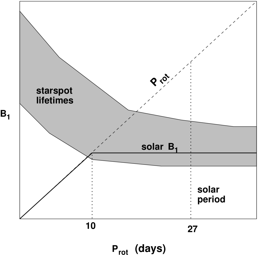
Figure 6: Schematic illustration of the expected dependence of the active regions component’s characteristic timescale $B_{1}$ on rotational period.

If the active regions component of micro-variability is the result of the rotational modulation of active regions, we expect $B_{1}$ to be directly related to the period. However, the value obtained for the Sun is $B_{1}=8.5\times 10^{6}$ s, i.e. $9.84$ days, compared to a rotational period of $\approx 26$ days. This suggests that the timescale is not (or not exclusively) dominated by rotational modulation of active regions, but by the emergence and disappearance of the structures composing the active regions. Individual active regions evolve on a timescale of weeks to months in the Sun (Radick et al., 1998), but spots and faculae evolve faster: observed sunspot lifetimes range roughly between 10 days and 2 months (Hiremath, 2002). We therefore deduce that sunspot evolution is the process which determines $B_{1}$ in the Sun.

This reasoning can be generalised in the following way: the phenomenon with the shortest timescale (in the relevant range) is expected to determine $B_{1}$. In the Sun, this phenomenon is sunspot evolution. As spot lifetimes are, if anything, longer in faster rotators (Barnes et al., 1998; Soon et al., 1999), rotational modulation should take over below a certain period. As a rough estimate we have placed the boundary between the two regimes at $P_{\rm rot}=10$ days (see Fig. 6).

This completes, within the obvious limits of the assumptions used, the requirements for the simulation of white light stellar light curves with micro-variability, within the range of applicability of the scaling laws used: $0.45\leq B-V\leq 1.3$, $t\geq t_{\mathrm{Hyades}}$, and the star must still be on the main sequence. The stellar parameters required are age (or rotation period) and $B-V$ colour (or spectral type). It is also possible to supply $A_{1}$ and $B_{1}$ directly. Once an artificial power spectrum is generated, phases drawn at random from a uniform distribution are applied before applying a reverse Fourier transform to return to the time domain.

Due to the use of randomly chosen phases, the shape of the variations does not resemble the observed solar variability. It may be possible to characterise the sequence of phases characteristic of a given type of activity-related event, such as the crossing of the stellar disk by a starspot, facula or active region. This information could then conceivably be included, with appropriate scaling, in the model, in order to make the shape of the variations more realistic. However, how to do this in practice is not immediately obvious, and will be investigated in the future. As the model stands, the simulated light curves can be used to estimate quantities such as amplitude, timescale, the distribution of residuals from a mean level, but no conclusions should be drawn from the shape of individual variations.

3.5 A few basic tests

Figure 7: Comparison of a portion of PMO6 data starting 1300 days after the start of the full light curve (top panel) with a simulated light curve generated using the Sun’s observed rotation period ($25.4$ days) and chromospheric activity index ($R^{\prime}_{\mathrm{HK}}=-4.89$, Radick et al. 1998). Both light curves have 15 min sampling, last 180 days and are normalised to a mean flux of $1.0$.

A first check is to compare the predicted observables for the Sun to the measured values. The measured period and $\log\left<R^{\prime}_{\mathrm{HK}}\right>$ are $25.4$ days and $-4.89$ (Radick et al., 1998), in good agreement with the predicted values of $23.4$ days and $-4.84$. The measured $\mathrm{rms}_{by}$ is $\simeq 5$ in units of $10^{-4}$ mag. The value measured from a simulated light curve with $1$ day sampling lasting $6$ months, when allowing for the conversion between $\mathrm{rms_{white}}$ and $\mathrm{rms}_{by}$ is $6.11$. This slight over-prediction is attributable to the Sun’s slightly slow rotation and low activity for its age and type, and to the fact that it is slightly under-variable for its activity level (it falls slightly below the fit on Fig. 5). Fig. 7 compares a portion of the PMO6 light curve taken from a relatively high activity part of the solar cycle with a light curve simulated using the observed rotation period and activity index of the Sun. The amplitude and typical timescales of the variations are well matched.

A set of six light curves have been simulated, corresponding to three spectral types (F5, G5 and K5) and two ages (625 Myr and 4.5 Gyr). Examination of the light curves and the various parameters computed during the modelling process can reveal any immediate discrepancies. The light curves are shown in Fig. 8 and the parameters in Table 2. They follow the expected trends, variability decreasing with age and $B-V$ and increasing with $P_{\mathrm{rot}}$, so that at a given age the least active star is the G star, while the most active is the K star, despite is long rotation period (due to the dependence of activity on colour).

Figure 8: Examples of simulated light curves containing micro-variability for Hyades age (left column) and solar age (right column) stars with spectral types F$5$ (top row), G$5$ (middle row) and K$5$ (bottom row). A single transit by a $0.5\leavevmode\nobreak\ R_{\mathrm{Jup}}$ planet has been added to each light curve 75 days after the start (a transit by an Earth-sized planet would be $\approx 25$ times smaller). The light curves have $1$ hr sampling and last 150 days.

Table 2: Parameters of the simulated light curves.

$$\begin{array}[]{llllllll}\hline\cr\vskip 3.0pt plus 1.0pt minus 1.0pt\cr\mathrm{Age}&\mathrm{SpT}&B-V&P_{\mathrm{rot}}&\log\left(R^{\prime}_{\mathrm{HK}}\right)&A_{1}&B_{1}&\mathrm{rms_{white}}\\ \mathrm{Gyr}&&&\mathrm{days}&&\times 10^{5}&\mathrm{days}&\times 10^{4}\\ \vskip 3.0pt plus 1.0pt minus 1.0pt\cr\hline\cr\vskip 3.0pt plus 1.0pt minus 1.0pt\cr 0.625&\mathrm{F}5&0.44&2.9&-4.64&19.27&2.89&22.0\\ 0.625&\mathrm{G}5&0.68&8.8&-4.44&38.16&8.80&46.5\\ 0.625&\mathrm{K}5&1.15&12.6&-4.42&41.40&9.84&69.5\\ 4.5&\mathrm{F}5&0.44&7.8&-5.23&4.66&7.87&13.3\\ 4.5&\mathrm{G}5&0.68&23.7&-4.80&11.95&9.84&13.9\\ 4.5&\mathrm{K}5&1.15&33.8&-4.67&17.53&9.84&14.4\\ \vskip 3.0pt plus 1.0pt minus 1.0pt\cr\hline\cr\end{array}$$

4 Impact of micro-variability on transit detection from space

A set of routines have been written to allow the rapid and automated generation of light curves containing variability, some or no transits, and photon noise, given the age and spectral type of the star, if applicable the radius, period and mass of the planet, and the expected photon count per sampling time. This allows the systematic exploration of the detection limits in the stellar and planetary parameter space for a given instrument.

For our study we have used the current configuration of the Eddington mission, as described by Favata (2003). The mission is currently (June 2003) in its detailed definition phase, so that the final payload configuration may evolve from the current baseline. Currently, the Eddington payload is constituted by a set of 4 identical wide field telescopes, with identical white light CCD cameras at the focal plane. In practice, this is equivalent to a single monolithic telescope with the same collecting area as the sum of the collecting areas of the 4 individual telescopes. The total collecting area of the baseline payload design is 0.764 m², and the field of view has a diameter of 6.7 deg. The CCD chips used will be from E2V and will have the standard “broad band” response. The mission is scheduled for a launch in early 2008, and will perform its terrestrial planet-finding program by observing a single region of the sky for three years without interruptions.

4.1 Which are the best target stars – Impact on the choice of planet-finding field

The aim here is to identify, for example, those stars which are likely to be so variable that the detection of terrestrial planets orbiting them by Eddington and Kepler will be seriously hindered, or on the contrary where the transits are easily recovered even in the presence of variability. This will be used to optimise both the choice target fields and the observing strategy, so that the range of apparent magnitudes containing most of the best target stars is well covered.

Light curves were therefore generated for a grid of star ages ($0.625$, $1.0$, $2.0$, $3.0$ & $4.5$ Gyr) and types (F$5$, F$8$, G$0$, G$2$, G$5$, G$8$, K$0$, K$2$ & K$5$). Planetary transits were added to the light curves for $1$ & $3\leavevmode\nobreak\ R_{\oplus}$ and $1\leavevmode\nobreak\ R_{\mathrm{Jup}}$ planets with periods of $30$ days, $6$ months, $1$ year and $3$ years, resulting in $37$, $7$, $3$ and $1$ transit(s) respectively. The light curves last $3$ years and have a sampling of $1$ hr. Photon noise was added as suitable for the current Eddington baseline design.Two apparent magnitudes, $V=13$ and $V=15$, were used.

Note that the expected sampling rate is in fact closer to 10 min than 1 hr. However, this first set of simulations was designed to rapidly explore the stellar parameter space to identify regions of interest. For this purpose, the light curves were generated using a longer integration time, thereby keeping them to a manageable size and maximising the contribution of stellar noise relative to photon noise on a given data point – the impact of photon noise having already been investigated in a previous paper (Aigrain & Favata, 2002). Later simulations, concentrating on the habitable zones of the more promising target stars, were made with 10 min sampling.

To estimate the detectability of the transits in each case, the light curves were first pre-processed using an optimal Wiener-like filter (Carpano et al., 2003). This has the effect of whitening the noise and increasing the signal to noise ratio of the transits. A transit detection algorithm based on a maximum likelihood approach with a simple box-shaped transit model (Irwin & Aigrain, 2003) was then applied to the filtered light curves. The results are shown in Figs. 10 & 11, using the notation described in Fig. 9. For each case, we have indicated whether the best candidate transit(s) (i.e. the set of trial parameters which gave rise to the minimum in the detection statistic), corresponds to the true transit(s) inserted in the light curve. Note that only one simulation was performed for each star-planet combination, and the results should therefore be taken as indicative rather than quantitative. The decision not to perform full Monte Carlo simulations at this stage was taken because both the variability model and the detection and filtering algorithms are still undergoing frequent improvements.

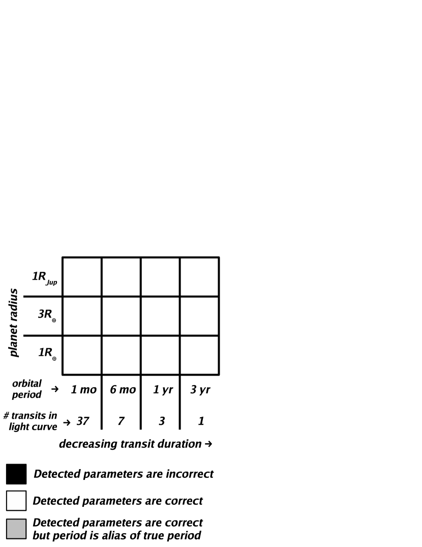
Figure 9: Notation used to present the results of the Eddington simulations.

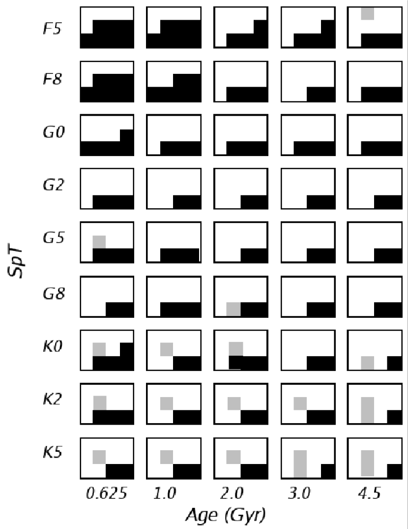
Figure 10: Results of the Eddington simulations with $1$ hr sampling and $V=13$. The notation used is detailed in Fig. 9.

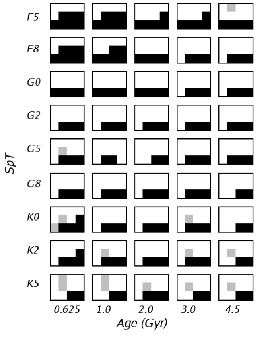
Figure 11: Results of the Eddington simulations with $1$ hr sampling and $V=15$. The notation used is detailed in Fig. 9.

The main conclusions to be drawn from these results are:

• The detection of transits by planets with $R_{\mathrm{pl}}\leq 3\leavevmode\nobreak\ R_{\oplus}$ around stars younger than $2.0$ Gyr or earlier than G$0$ is significantly impaired, and they are not good targets for the exo-planet search of Eddington or for Kepler.

• The small radius (hence increased transit depth) of K stars outweighs their relatively high variability levels, making them the best targets aside from effects not considered here, such as magnitude distribution and crowding. These will need to be assessed carefully. Whether this trend continues for M stars – recalling that they were not included in the simulations because of the significant number of fast M rotators present at Hyades age – is an open question (see Deeg, 2003). Another complicating factor for these late-type stars is the need to include the effects of micro- and nano-flaring, an issue under investigation.

• Earth-sized planets are not detected correctly around G stars with $3$ transits only. This is only an indicative result, but it demonstrates the need to increase the transit signal-to-noise ratio for such systems, i.e. the square root of the number of in-transit points times the signal-to-noise ratio per data point. As photon noise is not the limiting noise factor at $V=13$, increasing the collecting area would not achieve this. Instead, one needs to increase the number of in-transit points, while keeping the signal-to-noise ratio per data point constant. This can be achieved through longer light curve duration. Finer time sampling would increase the number of in-transit points, but also the photon noise per data point. It is thus expected to improve the results for the bright, stellar noise dominated stars. The magnitude limit between the stellar noise and photon noise dominated regimes depends on the integration time, so that the optimum sampling rate is likely to be magnitude dependent.

• At $V=15$ and with $1$ hr sampling, photon noise has become the dominant factor for most stars.

The third point in the list above could have important consequences for the target field/star selection for Kepler. The current target field is centred on a galactic latitude of $\simeq 5^{\circ}$ in the region of Cygnus, and was chosen to maximise the number of stars in the field while being sufficiently far from the plane of the ecliptic to allow continuous monitoring (Borucki et al., 1997). Due to telemetry constraints, which limit the number of observed stars to $\simeq 100\,000$, and to crowding, which can have a very large impact in such high density regions, only stars with $V\leq 14$ are likely to be monitored in this field. However, with its larger collecting area (corresponding to a single aperture of $0.95$ m), Kepler’s light curves will be star noise rather than photon noise dominated down to fainter magnitudes than in the case of Eddington. Given that, out of the spectral types tested here, K stars gave the best results, and that these stars tend to be fainter than earlier types, it may be desirable to choose a field at higher galactic latitude, combined with a deeper magnitude limit. It would likely be difficult to extend the magnitude limit while keeping the same target field due to increased crowding.

The final choice of target fields for both Eddington and Kepler will depend on many factors besides micro-variability and the change of stellar radii with spectral type, which are the only two effects taken into account in the present simulations. The constraints imposed by limited telemetry budgets, as well as the different apparent magnitude distributions of different stellar types, and the problems due to crowding in high density regions, have already been mentioned. It is only possible to characterise the spectral types of the stars in the field through multi-colour photometry – a necessary task if efficient target star selection is to be achieved, and one that would require very large amounts of telescope time if attempted spectroscopically – if patchy extinction is avoided. Full-sky surveys based on photographic plates, such as the Digitized Palomar Observatory Sky Survey (Djorgovski et al., 2002), can be used to detect regions of patchy extinction. Another important consideration is the availability of ground-based facilities accessible to the scientific community involved with each mission, for preparatory and follow-up observations. As the target field will be far from the ecliptic plane, it will be efficiently observable from either the southern or the northern hemisphere, but not both.

4.2 Minimum detectable transit in the presence of variability

Another question of interest is whether Eddington will really probe the habitable zone of the stars it targets, if micro-variability is taken into account. For this purpose, we have simulated light curves with increased sampling ($10$ min) for three $4.5$ Gyr old stars (types G$2$, K$0$ & K$5$) orbited by planets with radii of $0.8$, $1.0$, $1.5$ & $2.0\leavevmode\nobreak\ R_{\oplus}$, with periods of $180$, $360$ & $365$ days (corresponding to $7$, $4$ and $3$ transits in the light curves respectively). The last two have very similar periods (i.e. virtually identical transit shapes and durations) but the extra transit in the $360$ day case is due to the fact that the first transit occurs soon after the start of the observations. This is intended to test the effect of adding an extra year to the planet-search phase, in order to detect more transits.

The boundary between the stellar noise dominated and photon noise dominated regime, situated between $V=13$ and $V=15$ for 1 hr integration, will be approximately $1$ mag brighter for $10$ min integrations. In order to ensure that this second set of simulations still covered, at least in part, the stellar noise dominated regime, two values were used for the apparent magnitude of the stars: $V=12$ and $V=13$.

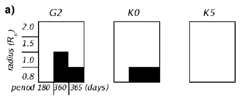
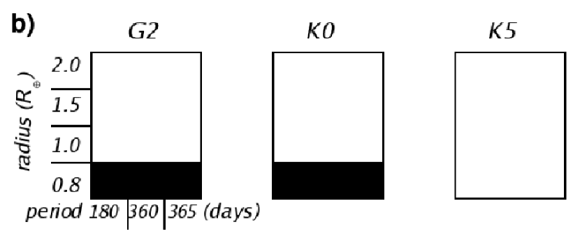
Figure 12: Results of the Eddington simulations with $10$ min sampling and apparent stellar magnitudes of $V=12$ (a) and $V=13$ (b).

The results are shown in Fig. 12. Generally speaking, they follow the expected trends. While the $0.8\leavevmode\nobreak\ R_{\oplus}$ planet is detected provided enough transits are present at $V=12$, it is not detected around all but the smallest star at $V=13$, as a result of the increased level of photon noise. The Earth-sized planet is only marginally detectable with 3 or 4 transits around a G$2$ star, even at $V=12$. The fact that it is detected with 4 transits but not with 3 at $V=12$, and is detected in both cases at $V=13$, highlights the need for full Monte Carlo simulations to obtain more reliable detectability estimates. It should serve as a reminder that the present work only aims to provide a global picture of the trends with star, planet and observational parameters, rather than quantitative results. Closer inspection of the light curve containing 4 Earth-sized transits around a G$2$ star at $V=12$ showed that two of them were superposed on parts of the light curve where the noise was consistently positive, which impeded the detection. The rate of such coincidences can only be estimated from multiple realisations of the same system. To summarise, in the stellar noise dominated regime, the minimum reliably detectable radii for G$2$, K$0$ and K$5$ stars are roughly $1.5$, $1.0$ and $0.8\leavevmode\nobreak\ R_{\oplus}$ respectively with 3 or 4 transits, and $0.8\leavevmode\nobreak\ R_{\oplus}$ in all cases with 7 transits.

By comparison, ‘habitable’ planets are usually required to have radii in the range $0.8\leavevmode\nobreak\ R_{\oplus}\leq R_{\mathrm{pl}}\leq 2.2\leavevmode\nobreak\ R_{\oplus}$. This choice of radii, based on the rationale of Borucki et al. (1997), corresponds to a mass range of $0.5$ to $10\leavevmode\nobreak\ M_{\oplus}$. Above $10\leavevmode\nobreak\ M_{\oplus}$, accretion of H and He starts and the planet will likely become a gaseous giant. Below $0.5\leavevmode\nobreak\ M_{\oplus}$, the planet is not able to retain a significant atmosphere, or to sustain plate tectonics on biologically significant timescales. They must also lie in the ‘habitable zone’. This zone is usually defined to ensure the existence of liquid water on the surface of the planet, the inner edge being due to loss of water through photolysis and hydrogen escape, and the outer edge to an increase in albedo which leads to a drop in surface temperature (Kasting et al., 1993). Franck et al. (2002) compute age-dependent habitable zone limits, requiring the surface temperature to be in the range $0$ to $100\leavevmode\nobreak\ ^{\circ}$C and taking into account the change in luminosity of a star while on the main sequence. They give the following orbital distance ranges for the habitable zones of $4.5$ Gyr old stars: $0.5$ to $1$ A.U. ($0.8\leavevmode\nobreak\ M_{\odot}$, K$2$ star) and $0.9$ to $1.3$ A.U. ($1.0\leavevmode\nobreak\ M_{\odot}$, G$2$ star). A similar but simplified calculation (K. Horne, priv. comm.) using a single luminosity value, and converting to period using the mass range $0.5$ to $10\leavevmode\nobreak\ M_{\oplus}$, yields the periods corresponding to the centre of the habitable zone as $1.2$, $0.6$ and $0.3$ years for G$2$, K$0$ and K$5$ stars respectively.

The effect of the increased sampling rate is immediately visible. While a ‘true Earth analogue’ (Earth-sized planet orbiting a G$2$ star with a period of $1$ year) may not be detected reliably, a good part of the habitable zone of the G$2$ star and all of that of the K$0$ and K$5$ stars are covered. This suggests that the primary goal of discovering and characterising extra-solar planets in the habitable zone will be achievable around intermediate age and old late-G and K stars with the current design. To push back these limits, modifications to the baseline design – such as the possible inclusion of colour information – are under study at present. The fact that the detectability of both $1.0$ and $0.8\leavevmode\nobreak\ R_{\oplus}$ planets increases significantly with increased number of transits, suggests that it may be desirable to increase the duration of the planet search stage, or to return to the planet search field for confirmation after a break (during which the asteroseismology programme, the other primary goal of Eddington, would be carried out).

4.3 Detection threshold definition

An interesting consequence of introducing non-Gaussian noise in the data is illustrated by these simulations. The fact that the detection was correct does not imply it would have been considered significant. Given a light curve in which there may or may not be one or more transits, some kind of threshold must be used, in order to automatically exclude candidate transits which are likely to be spurious. Theoretically, in the presence of Gaussian noise only, a global threshold can be used, i.e. a detected transit can be considered reliable if its signal to noise exceeds a certain value, whatever the star or planet parameters (Jenkins et al., 2002). However, the use of a single threshold (designed to keep the number of false alarms to 1 or less) in the present case leads to an alarmingly high rate of missed detections. In particular, almost all correctly detected transits by Earth-sized planets would be discarded because their signal to noise ratio is too low. This is presumably due to the non-Gaussian nature of the stellar noise. However, it is interesting to note that the detected duration is almost always the maximum trial value when the detected event is spurious. This suggests that the spurious events which mimic transits last, on average, longer than transits, and might be a pointer to a method for excluding most of the spurious events automatically. A possible solution to the S/N threshold problem might therefore be found by taking into account the duration of the detected event when computing a detection threshold – and applying a more stringent criterion to the longer duration events. This possibility will be investigated in the near future.

For the purposes of the present simulations, the correct or incorrect detection of the single realisation of a given star-planet system was taken as indicative of the detectability of such a system by Eddington. To evaluate more precisely expected detection limits once the planet finding field have been chosen, more detailed simulations can be carried out.

5 Conclusions

A model to generate artificial light curves containing intrinsic variability on timescales from hours to weeks for stars between mid-F and late-K spectral type and older than $0.625$ Myr has been presented. This model relies on the observed correlation between the weeks timescale power contained in total solar irradiance variations as measured by VIRGO/PMO6 and the Ca ii K-line index of chromospheric activity. The resulting light curves appear consistent with currently available data on variability levels in clusters and with solar data. Further testing and fine-tuning requires high sampling, long duration space-based stellar time-series photometry and will be carried out as such data become available.

The simulated light curves can be used to estimate the impact of micro-variability on exo-planet search missions such as Eddington and Kepler. The results of simulations including stellar micro-variability, photon noise as expected for Eddington and transits have been presented. After optimal filtering, the results of transit searches on these light curves suggest that stellar micro-variability, combined with the change in stellar radius with spectral type, will make the detection of terrestrial planets around F-type stars very difficult. On the other hand, K-stars appear to be promising candidates despite their high variability level, due to their small radius.

At $V=12$ and with $10$ min sampling, the smallest detectable planetary radii for $4.5$ Gyr old G$2$, K$0$ and K$5$ stars, given a total of 3 or 4 transits in the light curves, were found to be $1.5$, $1.0$ and $0.8\leavevmode\nobreak\ R_{\oplus}$ respectively. This result was obtained in stellar noise rather than photon noise dominated light curves, and therefore also applies to lower apparent magnitudes or larger collecting areas. The magnitude limit beyond which photon noise would start to dominate, thereby increasing the minimum detectable radii for a given star and observing configuration, depends on the collecting area and sampling time, but the effects of increased photon noise are detected at $V=13$ for $10$ min sampling time and Eddington’s collecting area.

All the simulated light curves produced so far, as well as the routines used to generate them, have been made available to the exo-planet community through the web page: www.ast.cam.ac.uk/~suz/simlc. Light curves with specific parameters can be generated on request. The inclusion of this model in the simulating tools under development for both missions is under study.

The next step is the extension of the model presented here to include colour information, to allow a detailed assessment of the pros and cons of including broadband filters on one or more of Eddington’s four telescopes. This will be the subject of an upcoming paper. At the same time, the performance of a range of filtering and transit detection algorithms, which have recently been compared in simulations including white noise only (Tingley, 2003), will be compared in the presence of micro-variability.