MAGNETIC BRAKING AND VISCOUS DAMPING OF DIFFERENTIAL ROTATION IN CYLINDRICAL STARS

Abstract

Differential rotation in stars generates toroidal magnetic fields whenever an initial seed poloidal field is present. The resulting magnetic stresses, along with viscosity, drive the star toward uniform rotation. This magnetic braking has important dynamical consequences in many astrophysical contexts. For example, merging binary neutron stars can form “hypermassive” remnants supported against collapse by differential rotation. The removal of this support by magnetic braking induces radial fluid motion, which can lead to delayed collapse of the remnant to a black hole. We explore the effects of magnetic braking and viscosity on the structure of a differentially rotating, compressible star, generalizing our earlier calculations for incompressible configurations. The star is idealized as a differentially rotating, infinite cylinder supported initially by a polytropic equation of state. The gas is assumed to be infinitely conducting and our calculations are performed in Newtonian gravitation. Though highly idealized, our model allows for the incorporation of magnetic fields, viscosity, compressibility, and shocks with minimal computational resources in a 1+1 dimensional Lagrangian MHD code. Our evolution calculations show that magnetic braking can lead to significant structural changes in a star, including quasistatic contraction of the core and ejection of matter in the outermost regions to form a wind or an ambient disk. These calculations serve as a prelude and a guide to more realistic MHD simulations in full 3+1 general relativity.

1. INTRODUCTION

Magnetic fields play a crucial role in determining the evolution of many relativistic objects. Some of these systems are promising sources of gravitational radiation for detection by laser interferometers now under design and construction, such as LIGO, VIRGO, TAMA, GEO, and LISA. For example, merging neutron stars can form a differentially rotating “hypermassive” remnant (Rasio & Shapiro 1992, 1999; Baumgarte, Shapiro, & Shibata 2000; Shibata & Uryū 2000). These configurations have rest masses that exceed both the maximum rest mass of nonrotating spherical stars (the TOV limit) and uniformly rotating stars at the mass-shedding limit (“supramassive stars”), all with the same polytropic index. This is possible because differentially rotating neutron stars can support significantly more rest mass than their nonrotating or uniformly rotating counterparts. Baumgarte, Shapiro & Shibata (2000), have performed dynamical simulations in full general relativity to demonstrate that hypermassive stars can be constructed that are dynamically stable against radial collapse and nonradial bar formation. The dynamical stabilization of a hypermassive remnant by differential rotation may lead to delayed collapse and a delayed gravitational wave burst. The reason is that the stabilization due to differential rotation, although expected to last for many dynamical timescales (i.e. many milliseconds), will ultimately be destroyed by magnetic braking and/or viscosity. These processes drive the star to uniform rotation, which cannot support the excess mass, and will lead to catastrophic collapse, possibly accompanied by some mass loss.

Baumgarte & Shapiro (2003) discuss several other relativistic astrophysical scenarios in which magnetic fields will be important. Neutron stars formed through core collapse supernovae are probably characterized by significant differential rotation (see, e.g., Zwerger & Müller 1997; Rampp, Müller, & Ruffert 1998; Liu & Lindblom 2001; Liu 2002, and references therein). Conservation of angular momentum during the collapse is expected to result in a large value of $\beta=T/|W|$, where $T$ is the rotational kinetic energy and $W$ is the gravitational potential energy. However, uniform rotation can only support small values of $\beta$ without leading to mass shedding (Shapiro & Teukolsky, 1983). Thus, nascent neutron stars from supernovae probably rotate differentially, giving magnetic braking and viscosity an important dynamical role. Short period gamma-ray bursts (GRB’s) are thought to result from binary neutron star mergers (Narayan, Paczynski, & Piran 1992) or tidal disruptions of neutron stars by black holes (Ruffert & Janka 1999). Meanwhile, long period GRB’s are believed to result from collapses of rotating massive stars to form black holes (MacFadyen & Woosley 1999). In most current models of GRB’s, the burst is powered by rotational energy extracted from the neutron star, black hole, or surrounding disk (Vlahakis & Konigl 2001). This energy extraction can be accomplished by strong magnetic fields, which also provide an explanation for the collimation of GRB outflows into jets (Meszaros & Rees 1997; Sari, Piran, & Halpern 1999; Piran 2002) and for the observed gamma-ray polarization (Coburn & Boggs 2003). The dynamics of supermassive stars (SMS’s), which may have been present in the early universe, will also depend on magnetic fields if the SMS’s rotate differentially. Loss of differential rotation support will affect the collapse of SMS’s, which has been proposed as a formation mechanism for supermassive black holes observed in galaxies and quasars, or their seeds (see Rees 1984, Baumgarte & Shapiro 1999, Bromm & Loeb 2003, and Shapiro 2003 for discussion and references). Finally, the effectiveness of the $r$-mode instability in rotating neutron stars may depend on magnetic fields. This instability has been proposed as a mechanism for limiting the angular velocities of neutron stars and for producing quasi-periodic gravitational waves (Andersson 1998; Friedman & Morsink 1998; Andersson, Kokkotas, & Stergioulas 1999; Lindblom, Owen, & Morsink 1998). Due to flux-freezing, however, the magnetic fields may distort or suppress the $r$-modes (see Rezzolla et al.  2000, 2001a,b and references therein).

Motivated in part by the growing list of important, unsolved problems which involve hydromagnetic effects in strong-field dynamical spacetimes, Shapiro (2000, hereafter Paper I) performed a simple, Newtonian, MHD calculation to highlight the importance of magnetic fields in differentially rotating stars. In this model, the star is idealized as a differentially rotating infinite cylinder consisting of a homogeneous, incompressible conducting gas in hydrostatic equilibrium. The magnetic field is taken to be purely radial initially and is allowed to evolve according to the ideal MHD equations. A constant shear viscosity is also allowed. Note that, though highly idealized, this model allows several important physical effects to be included in a 1+1 evolution code, requiring much less computational effort than more realistic 3+1 simulations.

Paper I presents results for the behavior of differentially rotating cylinders in three physical situations: zero viscosity with a vacuum exterior, nonzero viscosity with a vacuum exterior, and zero viscosity with a tenuous ambient plasma atmosphere. In the first case, for which the solution is analytic, the magnetic field gains a toroidal component which oscillates back and forth in a standing Alfvén wave pattern. The angular velocity profile oscillates around a state of uniform rotation, with uniform rotation occurring at times when the azimuthal magnetic field is at its maximum magnitude. At these times, a significant amount of the rotational energy has been converted to magnetic energy. In the absence of a dissipation mechanism, these oscillations continue indefinitely. In the second case (vacuum exterior with nonzero viscosity), the oscillations are damped and the cylinder is driven to a permanent state of uniform rotation with a significant fraction of its initial rotational energy having been converted into magnetic energy and finally into heat. In the final case (zero viscosity with a plasma atmosphere), Alfvén waves are partially transmitted at the surface and carry away significant fractions of the angular momentum and energy of the cylinder. In all of these situations, only the timescale, and not the qualitative outcome, of the dynamical behavior depends on the strength of the initial magnetic field. Thus, even for a small initial seed field, magnetic braking and viscosity eventually drive the cylinders toward uniform rotation.

The braking of differential rotation by magnetic fields is also currently being studied in a spherical, incompressible neutron star model (Liu & Shapiro, in preparation). This calculation treats the slow-rotation, weak-magnetic field case in which $T\ll E_{\rm mag}\ll|W|$, where $E_{\rm mag}$ is the total magnetic energy. Consequently, the star is spherical to a good approximation and poloidal velocities in the $\theta-$ and $r-$ directions can be neglected on the timescales of interest. Liu & Shapiro solve the MHD equations for the coupled evolution of the angular velocity $\Omega$ and the azimuthal magnetic field $B_{\phi}$ in both Newtonian gravity and general relativity. The resulting angular velocity and poloidal field profiles often develop rich small-scale structure due to the fact that the eigenfrequencies of $B_{\phi}$ vary with location inside the star.

In many cases, the loss of differential rotation support due to magnetic braking is expected to lead to interesting dynamical behavior. In hypermassive stars, magnetic braking may lead to catastrophic gravitational collapse. In general, however, one expects a range of radial motions, including oscillations, quasistatic contraction, and ejection of winds. These behaviors are not present in the results of Paper I because of the assumptions of homogeneity and incompressibility. In that case, no radial velocities occur as the system evolves away from equilibrium. In the present paper, we explore the effects of compressibility by generalizing the calculations of Paper I to Newtonian cylindrical polytropes. Though other aspects of the present model are again highly idealized, allowing for compressible matter results in a much more realistic spectrum of dynamical behavior, including radial contraction, mass ejection, and shocks. By formulating the problem in 1+1 dimensions and working in Lagrangian coordinates, we are able to solve the MHD equations essentially to arbitrary precision. Our simulations again serve to identify most of the key physical and numerical parameters, scaling behavior, and competing timescales associated with magnetic braking and differential rotation. The structure of this paper is as follows: Section 2 describes our basic model. In Section 3, we discuss the structure of equilibrium cylindrical polytropes which serve as initial data for our evolution calculations. In Section 4, we set out the fundamental MHD evolution equations and put them in a convenient nondimensional form. Section 5 describes the results of MHD evolution calculations for several choices of the parameters which serve to illustrate the effects of compressibility and differential rotation. We discuss the significance of these calculations in Section 6.

2. BASIC MODEL

As discussed in Paper I, differential rotation in a spinning star twists up a frozen-in, poloidal magnetic field, creating a very strong toroidal field. This process will generate Alfvén waves, which can redistribute the angular momentum of a star on timescales less than $\sim~{}100\,{\rm s}\,(10^{12}{\rm G}/B_{0})$, where $B_{0}$ is the characteristic initial poloidal field. Shear viscosity also redistributes angular momentum. However, molecular viscosity in neutron star matter operates on a typical timescale of $\sim~{}10^{9}{\rm s}$ in a star of $\sim~{}10^{9}{\rm K}$, so it alone is much less effective in bringing the star into uniform rotation than magnetic braking, unless the initial magnetic field is particularly weak. Turbulent viscosity, if it arises, can act more quickly.

We wish to track the evolution of differential rotation and follow the competition between magnetic braking and viscous damping. Following Paper I, we model a spinning star as an infinite, axisymmetric cylinder with a vacuum exterior. We adopt cylindrical coordinates $(r,\phi,z)$, with the $z-$ axis aligned with the rotation axis of the star, and assume translational symmetry in the $z-$ direction. We take the magnetic field to have components only in the $r-$ and $\phi-$ directions. The fluid is assumed to be perfectly conducting everywhere (the ideal MHD regime). In some of our models, we allow for the presence of a constant shear viscosity. For protoneutron stars with $T\gtrsim 10^{9}K$, the coefficient of bulk viscosity, due to the time lag for reestablishing beta equilibrium following a change in density, becomes comparable to the shear viscosity coefficient (Sawyer 1989). We do not account for bulk viscosity, however, since our models are strongly differentially rotating (and hence have large amounts of shear), while large scale density changes in our evolution calculations occur quasistatically (see Section 5).

To construct initial data for our dynamical simulations, we assume a polytropic equation of state (EOS): $P=K\rho^{\Gamma}$. The equations of hydrostatic equilibrium are then solved with an assumed form for the initial differential rotation law (discussed in Section 3). We take the $\phi-$ component of the magnetic field to be zero initially. We then evolve the system by numerically integrating the full set of coupled MHD equations. We allow for heating due to shocks and viscous dissipation during the evolution, and assume a $\Gamma-$law EOS, $P=(\Gamma-1)\rho\varepsilon$, where $\varepsilon$ is the specific internal energy.

3. EQUILIBRIUM CYLINDRICAL POLYTROPES

Here we discuss the initial data for our simulations. We derive the equations for the static case, and then generalize to include rotation and radial magnetic fields. Finally, we derive a virial relation for equilibrium infinite cylindrical stars, discuss the stability of these models to radial perturbations, and construct some numerical models.

3.1. Static Polytropes

The fundamental equations for a static polytrope are the polytropic EOS

$$P=K\rho^{\Gamma}=K\rho^{1+\frac{1}{n}},$$ (1)

where $\rho$ is the density, $P$ is the pressure, $K$ and $\Gamma$ are constants, and $n$ is the polytropic index, and the equation of hydrostatic equilibrium

$$\frac{1}{\rho}{\mathbf{\nabla}}P=-{\mathbf{\nabla}}\Phi,$$ (2)

where $\Phi$ is the Newtonian gravitational potential, which satisfies Poisson’s equation,

$$\nabla^{2}\Phi=4\pi\rho.$$ (3)

Note that we will work in units such that $G=1$. To find ${\mathbf{\nabla}}\Phi$, we first define $\mu(r)$ to be the mass per unit length interior to radius $r$. This gives

$$\mu(r)=2\pi\int_{0}^{r}\rho(r^{\prime})r^{\prime}dr^{\prime}.$$ (4)

Integrating equation (3) and imposing regularity at the origin yields

$$\frac{d\Phi}{dr}=\frac{2\mu(r)}{r}.$$ (5)

Differentiating equation (2) in cylindrical radius $r$ and combining with equation (3) yields

$$\frac{d}{dr}\left(\frac{r}{\rho}\frac{dP}{dr}\right)=-4\pi\rho(r)r.$$ (6)

This equation can be generalized for infinite planar or spherical geometries through similar arguments. The result is

$$\frac{d}{dr}\left(\frac{r^{\alpha-1}}{\rho}\frac{dP}{dr}\right)=-4\pi\rho(r)r^{\alpha-1},$$ (7)

where $\alpha=1,2,3$ corresponds to planar, cylindrical, and spherical geometry respectively.

We will make use of a common nondimensionalization of equation (7) to facilitate numerical solutions. We define nondimensional quantities according to

$$\rho = \rho_{c}\theta^{n}$$

$$r = a\xi$$ (8)

$$a = \left[\frac{(n+1)K\rho_{c}^{(1/n-1)}}{4\pi}\right]^{1/2},$$

where $\rho_{c}$ is the central density. Equation (7) then becomes a generalized Lane-Emden equation,

$$\frac{1}{\xi^{\alpha-1}}\frac{d}{d\xi}\left(\xi^{\alpha-1}\frac{d\theta}{d\xi}\right)=-\theta^{n}.$$ (9)

Hereafter we will treat $\alpha=2$ (cylindrical geometry). Spherical polytropes were described extensively by Chandrasekhar (1939); planar polytropes were constructed by Shapiro (1980). The boundary conditions on equation (9) are easily obtained from physical arguments. From equation (8), it is evident that $\theta(0)=1$. The condition on $\theta^{\prime}$ is obtained by using the fact that $\rho\to\rho_{c}$ so that equation (4) implies $\mu(r)\propto r^{2}$ as $r\to 0$, hence equations (1), (2), and (5) yield $d\rho/dr=0$, and hence $\theta^{\prime}(0)=0$. The equations should be integrated from the origin out until $\theta=0$, which implies $P=0$. This point is the surface of the star and will be denoted by $\xi_{1}$. This gives the pressure and density profiles for equilibrium configurations. Some analytic solutions to equation (9) are, for $n=0$, $\theta=1-\xi^{2}/4$ and for $n=1$, $\theta=J_{0}(\xi)$, where $J_{0}$ is the Bessel function of order zero.

3.2. Rotating Cylindrical Polytropes

We will now extend the cylindrical polytrope model to include the effects of rotation. The hydrostatic equilibrium equation is modified by a term accounting for centrifugal acceleration. The result is

$$\frac{1}{\rho}\frac{dP}{dr}=-\frac{d\Phi}{dr}+\Omega^{2}(r)r,$$ (10)

where $\Omega(r)$ is the angular velocity at radius $r$ (the $r$-dependence allows for differential rotation). Performing the same manipulations used to get equation (6) gives

$$\frac{d}{dr}\left(\frac{r}{\rho}\frac{dP}{dr}\right)=2\Omega^{2}r+r^{2}\frac{d\Omega^{2}}{dr}-4\pi\rho r.$$ (11)

Using the same nondimensionalization as equation (8) and making the definition

$$\zeta\equiv\frac{\Omega^{2}}{\pi\rho_{c}},$$ (12)

gives the cylindrical Lane-Emden equation with rotation,

$$\frac{d^{2}\theta}{d\xi^{2}}+\frac{1}{\xi}\frac{d\theta}{d\xi}+\theta^{n}-\frac{\zeta}{2}-\frac{\xi}{4}\frac{d\zeta}{d\xi}=0.$$ (13)

By identical reasoning, this equation has the same boundary conditions as equation (9).

There are two analytic solutions for uniform rotation ($\zeta={\rm constant}$). The analytic solutions are for $n=0$, $\theta(\xi)=1-(1-\zeta/2)\xi^{2}/4$ and for $n=1$, $\theta(\xi)=(1-\zeta/2)J_{0}(\xi)+\zeta/2$. In the rest of the paper, we will adopt the following $\Omega$ profile

$$\Omega(r)=\frac{\Omega_{0}}{2}\left[1+\cos\left(\frac{\pi r^{2}}{R^{2}}\right)\right],$$ (14)

where $R$ is the radius of the star. Letting $\zeta_{0}=\Omega_{0}^{2}/\pi\rho_{c}$ gives the nondimensional form

$$\zeta(\xi)=\frac{\zeta_{0}}{4}\left[1+\cos\left(\frac{\pi\xi^{2}}{\xi_{1}^{2}}\right)\right]^{2}.$$ (15)

Though this rotation law was chosen arbitrarily, it satisfies the boundary condition given below (eq. [45]) and has the expected property that $\Omega$ decreases monotonically with $r$. Shibata and Uryū (2000) found that hypermassive binary merger remnants typically have $\Omega(0)/\Omega(R)\approx 3$. Slightly modifying our rotation law to satisfy this condition resulted in a set of models qualitatively similar to those discussed below, usually with slightly larger allowed values of $\beta=T/|W|$. To solve equation (13) for rotation profile of equation (15), we must iterate our solutions to equation (13) to identify $\xi_{1}$, the surface radius of our star. As will be shown later, these equilibrium solutions are also valid for cylinders with radial magnetic fields, so we will use these solutions as initial data for our dynamical evolutions. We remark how simple it is to construct differentially rotating, infinite cylindrical polytropes, described by ordinary differential equations in one dimension, in comparison to finite rotating stars, which are defined by partial differential equations in two dimensions (see e.g. Tassoul 1978).

3.3. Virial Theorem and Stability

We will use the virial theorem to check the results of our equilibrium calculations and, later on, to test whether a configuration has reached a new equilibrium state following dynamical evolution. With the definitions

$$W \equiv -\int\rho{\mathbf{x}}\cdot{\mathbf{\nabla}}\Phi d^{3}x,$$

$$T \equiv \frac{1}{2}\int\rho\upsilon^{2}d^{3}x,$$ (16)

$$\Pi \equiv \int Pd^{3}x,$$

the virial theorem for an infinite cylindrical equilibrium star is

$$2T+W+2\Pi=0.$$ (17)

Notice that the numerical coefficients in this equation differ from the analogue for bounded configurations. (For a derivation, see Appendix A.) Also note that as shown in Appendix A, even if magnetic fields are present, this equation still holds unmodified for equilibrium stars. In our case it is convenient to write $d^{3}x=Ld\mathcal{A}=2\pi Lrdr$, where $L$ is an arbitrary length in the $z$-direction. We divide each quantity in equation (16) by $L$ to obtain quantities per unit length (we will continue to use the symbols $W$, $T$, and $\Pi$). Hereafter, we will refer to all extensive quantities as quantities per unit length in the $z-$ direction. These definitions give an identical virial theorem to equation (17). Using equations (4) and (5), the definition of $W$ can be integrated analytically to give

$$W=-\mu_{t}^{2},$$ (18)

where $\mu_{t}=\mu(R)$ is the total mass per unit length of the star.

The virial theorem can be used to find an upper limit on $\beta=T/|W|$ for any equilibrium cylindrical star. Since the pressure is always positive, $\Pi$ is positive definite. Similarly, $\mu_{t}^{2}$ is positive definite, so $W$ is negative or $W=-|W|$. Using these facts in equation (17) implies that for any equilibrium star

$$\beta\leq\frac{1}{2}.$$ (19)

We require our equilibrium solutions to be initially stable to radial perturbations to ensure that we are seeing the secular effects of magnetic fields in the evolution and not a hydrodynamical radial instability. For cylinders, the critical $\Gamma$ for stability is $\Gamma\geq 1$, permitting any $n\geq 0$ (see Appendix B). For spheres, however, one needs $\Gamma\geq 4/3$, which in turn requires $n\leq 3$. Note that rotation lowers the critical $\Gamma$, which does not change the limit on $n$, since any realistic EOS allows us to restrict ourselves to $n\geq 0$. Also note that the presence of a radial magnetic field does not affect this stability analysis, as shown in Appendix B.

3.4. Equilibrium Models

Here we present the results of our equilibrium model calculations. We write equation (13) as a system of two coupled first order ODE’s and integrate using a fourth order Runge-Kutta method. Below we discuss the comparison with an analytic Roche model for centrally condensed rotating cylinders and give a table of data for cylindrical polytropes.

3.4.1 Roche Model

The Roche model holds for uniformly rotating, centrally condensed, polytropic cylinders. Our discussion is patterned after Shapiro & Teukolsky (1983). We will show below that this approximate model improves with increasing $n$, as expected. Equation (10) may be written as

$$\frac{1}{\rho}\nabla P+\nabla(\Phi+\Phi_{c})=0,$$ (20)

where $\Phi_{c}=-\Omega^{2}r^{2}/2$. Because of the central condensation, near the surface $\mu\to\mu_{t}$ and

$$\frac{\partial\Phi}{\partial r}\simeq\frac{2\mu_{t}}{r}\Rightarrow\Phi\simeq 2\mu_{t}\ln r.$$ (21)

The specific enthalpy of a polytrope is given by

$$h(r)=\int^{r}dr^{\prime}\frac{1}{\rho}\frac{\partial P}{\partial r^{\prime}}=\frac{\Gamma}{\Gamma-1}\frac{P}{\rho}.$$ (22)

Equation (20) can now be integrated to obtain

$$h(r)+\Phi(r)+\Phi_{c}(r)=K,$$ (23)

where $K$ is an integration constant. Since the star is very centrally condensed and equation (23) holds throughout the envelope, $K$ is assumed to be the same as in the nonrotating case. Let $R_{0}$ be the radius of the nonrotating star. Then, since the enthalpy vanishes at the surface,

$$\Phi(R_{0})=K=2\mu_{t}\ln R_{0}.$$ (24)

A stable rotating star (i.e. not shedding mass) must have a radius $R_{1}$ such that $h(R_{1})=0$. Let the effective potential be defined as $\Phi_{\rm eff}=\Phi+\Phi_{c}$ and let the maximum of the effective potential be $\Phi_{\rm max}$. Then using equation (23) and the fact that $h(r)$ has a zero, this stability condition becomes

$$\Phi_{\rm max}\geqslant K,$$ (25)

where $\Phi_{\rm max}$ is determined by setting $\partial\Phi_{\rm eff}/\partial r=0$, giving

$$r=\sqrt{\frac{2\mu_{t}}{\Omega^{2}}}.$$ (26)

Inserting this value into $\Phi_{\rm max}$ gives the rotational stability condition

$$-\mu_{t}+2\mu_{t}\ln\sqrt{\frac{2\mu_{t}}{\Omega^{2}}}\geqslant 2\mu_{t}\ln R_{0}.$$ (27)

This implies that to avoid mass shedding, the star must satisfy

$$\Omega^{2}\leqslant\frac{2}{e}\frac{\mu_{t}}{R_{0}^{2}}$$ (28)

Then in terms of nondimensional variables of the nonrotating star, the stability criterion in the Roche approximation becomes

$$\zeta\leqslant-\frac{1}{e}\frac{4}{\xi_{1}}\left.\frac{\partial\theta}{\partial\xi}\right|_{\xi=\xi_{1}},$$ (29)

employing equations (5), (12), and (28). Now, we use our code to find the maximum $\zeta$ for solutions to equation (13) and compare to the Roche model results. We denote the maximum $\zeta$ from our code as $\zeta_{m}$ and the maximum $\zeta$ from the Roche model, equation (29), as $\zeta_{R}$. We find the following sets $(n,\zeta_{m},\zeta_{R})$: (1.0, 0.57425, 0.31767), (3.0, 0.10948, 0.08527), (5.0, 0.02977, 0.02659), and (10.0, 0.001795, 0.001767). These results confirm that the Roche model becomes increasingly more accurate as $n$ increases and the degree of central concentration increases.

3.4.2 Numerical Results

Table 1

Static Cylindrical Polytropes

$n$	$\xi_{1}$	$-\xi_{1}\left(\frac{d\theta}{d\xi}\right)_{\xi_{1}}$	$\rho_{c}/\bar{\rho}$
0.0	2.0	2.0	1.0
1.0	2.405	1.248	2.316
2.0	2.921	0.925	4.611
3.0	3.574	0.740	8.629
5.0	5.428	0.532	27.67

Table 1 summarizes numerical results for static cylindrical polytropes. As $n$ increases, the star becomes more centrally condensed. However, this is much less pronounced than in the spherical case, where $n=3$ gives $\rho_{c}/\bar{\rho}=54.18$ compared to $\rho_{c}/\bar{\rho}=8.629$ for cylinders. Table 2 gives the key results for uniformly rotating cylindrical polytropes spinning at the mass-shedding limit. Note that we have not found a maximum $n$ for solutions with finite $\mu_{t}$ in the case of cylindrical polytropes. In contrast, polytropic spheres with $n>5$ extend to infinite radius with infinite mass (Chandrasekhar 1939). An important consequence of our differential rotation law is that for $n\gtrsim 1.2$, we can get a larger value of $\beta$ than the maximum $\beta$ for uniform rotation, $\beta_{\rm max}$. Since we expect viscosity and magnetic braking to drive differential rotation toward uniform rotation, we expect the most interesting cases to be those where the star is forbidden to simply relax to uniform rotation. Figure 1 shows a plot $\beta_{\rm max}$ versus $n$, where we have marked the cases we dynamically evolve below after incorporating magnetic fields and viscosity. We expect the cases falling below the curve to relax to a uniformly rotating equilibrium polytrope and the cases above the curve to undergo major changes away from polytropic behavior.

Figure 1.— Maximum $\beta=T/|W|$ attainable for uniformly rotating stars (mass shedding limit; the solid line) and the values of $\beta$ which we will evolve numerically (marked with crosses and labeled I-VI). Note that the virial theorem sets the limit $\beta\leq 0.5$ for any equilibrium configuration.

Table 2

Maximally Rotating Cylindrical Polytropes

	Uniform Rotation		Differential Rotation
n	$\beta_{max}$	$\Omega_{max}/\sqrt{\pi\rho_{c}}$	$\beta_{max}$	$\Omega_{max}/\sqrt{\pi\rho_{c}}$
0.0	0.500	1.414	0.086	1.414
0.01	0.496	1.402	0.087	1.414
1.0	0.228	0.758	0.179	1.414
3.0	0.062	0.331	0.299	1.414
5.0	0.015	0.172	0.368	0.382

^a The maximum corresponds to the mass shedding limit.

^b Assumes the particular rotation law $\Omega~{}=~{}\frac{\Omega_{0}}{2}\left[1+\cos\left(\frac{\pi r^{2}}{R^{2}}\right)\right]$ and a monotonically decreasing density profile.

4. MHD EQUATIONS

We now assemble the fundamental equations for our MHD simulations. First, the fluid obeys the continuity equation,

$$\frac{\partial\rho}{\partial t}+{\mathbf{\nabla}}\cdot(\rho{\mathbf{v}})=0.$$ (30)

The fluid motion is governed by the magnetic Navier-Stokes equation:

$$\frac{\partial{\mathbf{v}}}{\partial t}+({\mathbf{v}}\cdot{\mathbf{\nabla}}){\mathbf{v}} = -\frac{1}{\rho}{\mathbf{\nabla}}P-{\mathbf{\nabla}}\Phi+\frac{{(\mathbf{\nabla}}\times{\mathbf{B}})\times{\mathbf{B}}}{4\pi\rho}$$ (31)

$$+\frac{\eta}{\rho}(\nabla^{2}{\mathbf{v}}+\text@frac{1}{3}{\mathbf{\nabla}}({\mathbf{\nabla}}\cdot{\mathbf{v}})),$$

where $\mathbf{B}$ is the magnetic field and $\eta$ is the coefficient of dynamic viscosity, which is related to the familiar kinematic viscosity according to $\nu=\eta/\rho$. We note that if ${\mathbf{B}}=0=\eta$, and $\mathbf{v}=\mathbf{\Omega}\times\mathbf{r}$, $\mathbf{\Omega}=\Omega\mathbf{\hat{z}}$, equation (31) reduces to the hydrostatic equilibrium equation for rotating cylinders (eq. [10]). The magnetic field $\mathbf{B}$ satisfies Maxwell’s constraint equation

$$\mathbf{\nabla}\cdot\mathbf{B}\ =\ 0,$$ (32)

as well as the flux-freezing equation

$${\partial\mathbf{B}\over\partial t}\ =\ \mathbf{\nabla}\times(\mathbf{v}\times\mathbf{B}).$$ (33)

Solving equation (32) for the magnetic field together with the flux-freezing condition (33) requires that the radial component of the magnetic field be independent of time and given by

$$B_{r}={B_{0}R\over r},~{}~{}~{}t\geq 0,$$ (34)

where $B_{0}$ is the value of the field at the stellar surface at $t=0$. Although the magnetic field given by equation (34) exhibits a static line singularity along the axis at $r=0$, it does not drive singular behavior in the fluid velocity or nonradial magnetic field. As these quantities, which are the main focus here, remain finite and evolve in a physically reasonable fashion, the line singularity poses no difficulty and requires no special treatment. Also, since the magnetic term in equation (eq. [31]) is proportional to the curl of $\mathbf{B}$, the radial magnetic field does not enter the hydrostatic equilibrium equation. Thus, the presence of an initially radial magnetic field does not affect the initial data equilibrium models described in Section 3. The virial theorem derived by taking a moment of equation (31) is identical to equation (17), which applies in the ${\mathbf{B}}=0$ case. (The magnetic field terms cancel as described in Appendix A.) Note that the virial theorem only holds for equilibrium configurations and is not expected to be satisfied during a dynamical evolution.

We next consider the properties of the fluid itself. The equation of state, $P=(\Gamma-1)\rho\varepsilon$, allows the entropy of a fluid element to increase if there is heating due to shocks or shear viscosity. The evolution of the specific internal energy is described by the First Law of Thermodynamics,

$$\frac{d\varepsilon}{dt}=-P\frac{d}{dt}\left(\frac{1}{\rho}\right)+T\frac{ds}{dt},$$ (35)

where the Lagrangian derivative is defined as $d/dt\equiv\partial/\partial t+{\mathbf{v}}\cdot\nabla$ and $s$ is the specific entropy. The rate of energy generation due to viscosity is given by

$$T\frac{ds}{dt}=\frac{1}{\rho}\sigma^{\prime}_{ij}\frac{\partial\upsilon_{i}}{\partial x_{j}},$$ (36)

where $\sigma^{\prime}_{ij}$ is the viscous stress tensor (Landau & Lifshitz 1998, eq. 15.3)

$$\sigma^{\prime}_{ij}=\eta\left(\frac{\partial\upsilon_{i}}{\partial x_{j}}+\frac{\partial\upsilon_{j}}{\partial x_{i}}-\text@frac{2}{3}\delta_{ij}\frac{\partial\upsilon_{k}}{\partial x_{k}}\right),$$ (37)

and where summation over repeated indices is implied.

We will now write our system of evolution equations in component form in Lagrangian coordinates (we work in an orthonormal basis). First, we define $j$ as the specific angular momentum: $j\equiv r\upsilon_{\phi}$, where $\upsilon_{\phi}$ is the $\phi-$ component of the velocity. We also explicitly use the gradient of $\Phi$ given in equation (5). Then equations (30), (31), (33), (35), and (36) become

$$\frac{d\rho}{dt} = -\frac{\rho}{r}\frac{\partial}{\partial r}(r\upsilon_{r})$$ (38)

$$\frac{d\upsilon_{r}}{dt} = -\frac{1}{\rho}\frac{\partial P}{\partial r}-\frac{2\mu}{r}+\frac{j^{2}}{r^{3}}-\frac{1}{8\pi\rho r^{2}}\frac{\partial}{\partial r}(r^{2}B_{\phi}^{2})$$ (39)

$$\mbox{}+\frac{4\eta}{3\rho}\frac{\partial}{\partial r}\left(\frac{1}{r}\frac{\partial(r\upsilon_{r})}{\partial r}\right)$$

$$\frac{dj}{dt} = \frac{B_{r}}{4\pi\rho}\frac{\partial}{\partial r}(rB_{\phi})+\frac{\eta r}{\rho}\frac{\partial}{\partial r}\left(\frac{1}{r}\frac{\partial j}{\partial r}\right),$$ (40)

$$\frac{dB_{\phi}}{dt} = -B_{\phi}\frac{\partial\upsilon_{r}}{\partial r}+rB_{r}\frac{\partial}{\partial r}\left(\frac{j}{r^{2}}\right),$$ (41)

$$\frac{d\varepsilon}{dt} = -\frac{P}{\rho^{2}}\left(\frac{d\rho}{dt}\right)+\frac{\eta r^{2}}{\rho}\left(\frac{\partial}{\partial r}\left(\frac{j}{r^{2}}\right)\right)^{2}$$ (42)

$$\mbox{}+\frac{2\eta}{9\rho}\left[\left(2\frac{\partial\upsilon_{r}}{\partial r}-\frac{\upsilon_{r}}{r}\right)^{2}+r^{4}\left(\frac{\partial}{\partial r}\left(\frac{\upsilon_{r}}{r^{2}}\right)\right)^{2}\right.$$

$$\left.\mbox{}+\frac{1}{r^{2}}\left(\frac{\partial(r\upsilon_{r})}{\partial r}\right)^{2}\right].$$

The terms on the r. h. s. in equation (42) involving derivatives of $\upsilon_{r}$ and $j$ represent heating due to the presence of shear viscosity. We note that the heating terms which depend on $\upsilon_{r}$ would not be present for an incompressible fluid. To handle shocks, we supplement the pressure by an artificial viscosity term: $P\to P+q$, where the recipe for $q$ is described in Appendix C.

4.1. Initial Conditions and Boundary Values

We assume that no azimuthal component of the magnetic field is present initially,

$$B_{\phi}(0,r)=0,\,\,\,\,r\geq 0,$$ (43)

recalling that $B_{r}$ is always given by equation (34). We are thus interested in the situation where the azimuthal field is created entirely by the differential rotation of the fluid, which bends the frozen-in, initially radial field lines in the azimuthal direction. Since the region outside of the cylinder is a vacuum, no azimuthal magnetic field can be carried into this region. Thus, $B_{\phi}$ must vanish at the surface:

$$B_{\phi}(t,R)=0,\,\,\,\,t\geq 0.$$ (44)

Together with equation (41), this implies

$$\frac{\partial}{\partial r}\left(\frac{j(t,R)}{r^{2}}\right)=0,\,\,\,\,t\geq 0.$$ (45)

The angular velocity $\Omega=j/r^{2}$ must be finite at the origin. This implies that $j(t,0)=0$ for all time. Also, since the cylinder is axisymmetric, the radial velocity at the origin must vanish for all time: $\upsilon_{r}(t,0)=0$. Since we begin our evolutions with an equilibrium cylindrical polytrope model, we take the radial velocity to be initially zero everywhere, that is, $\upsilon_{r}(0,r)=0$.

We now consider the boundary conditions on the fluid variables at the free surface of the cylinder, $r=R$. Pressure and density must both vanish at this surface:

$$\rho(t,R) = 0$$ (46)

$$P(t,R) = 0,\,\,\,\,t\geq 0.$$

When a viscosity is present, the free surface imposes an additional condition. Let ${\mathbf{n}}$ be the unit normal vector to the surface. Then, at the free surface, balance of forces requires that

$$-Pn_{i}+\sigma^{\prime}_{ij}n_{j}=0,$$

(Landau & Lifshitz 1998, eq. 15.16). Since ${\mathbf{n}}$ is radial and $P=0$ on the surface of the cylinder, this condition becomes $\sigma^{\prime}_{rr}=\sigma^{\prime}_{r\phi}=0$. Written in component form, $\sigma^{\prime}_{r\phi}=0$ becomes equation (45) and $\sigma^{\prime}_{rr}=0$ becomes

$$2\frac{\partial}{\partial r}\upsilon_{r}(t,R)-\frac{1}{r}\upsilon_{r}(t,R)=0,\,\,\,\,t\geq 0.$$ (47)

4.2. Conserved Energy and Angular Momentum

The magnetic Navier-Stokes equation (eq. [31]) admits two nontrivial integrals of the motion, one expressing conservation of energy and the other conservation of angular momentum of the star. Energy conservation may be expressed as

$$E(t)\ = E_{\rm kin}(t)\ +\ E_{\rm mag}(t)\ +\ E_{\rm int}(t)\ +\ E_{\rm grav}(t)$$ (48)

$$= E(0),$$

where $E_{\rm kin}(t)$ is the kinetic energy of the matter, $E_{\rm mag}(t)$ is the azimuthal magnetic energy, $E_{\rm int}(t)$ is the internal (thermal) energy, and $E_{\rm grav}(t)$ is the gravitational potential energy. These contributions are as follows:

$$E_{\rm kin}(t) = \text@onehalf\int d\mathcal{A}\rho(t,r)\left(\upsilon_{r}^{2}(t,r)+\frac{j^{2}(t,r)}{r^{2}}\right),$$

$$E_{\rm mag}(t) = \int d\mathcal{A}\frac{B^{2}_{\phi}(t,r)}{8\pi},$$

$$E_{\rm int}(t) = \int d\mathcal{A}\rho(t,r)\varepsilon(t,r),$$

$$E_{\rm grav}(t) = \text@onehalf\int d\mathcal{A}\rho(t,r)\Phi(t,r),$$ (49)

where $\Phi(t,r)$ is the gravitational potential, $d\mathcal{A}=2\pi rdr$, and all energies are taken per unit length as in Section 3.3. Equation (48) is derived by rewriting the Eulerian time derivative of the total energy density using equations (30), (31), and (35) and applying the divergence theorem. There is no explicit contribution from viscous heating in equation (48) because the internal energy, $E_{\rm int}$, accounts for this. We note that $E_{\rm grav}(t)$ is not the same as the gravitational term $W$ appearing in the virial theorem for equilibrium cylinders, which is defined according to equation (16). By contrast, $E_{\rm grav}(t)=W$ for spherical stars (Shapiro & Teukolsky 1983). Due to the cylindrical geometry of the present problem, $W$ cannot be identified as the gravitational potential energy. However, the ratio $T/|W|$, involving quantities from the virial theorem, can still be taken as a measure of the degree of rotation for a given mass per unit length.

Conservation of angular momentum per unit length is expressed as

$$J(t)\ =\int d\mathcal{A}\rho(t,r)j(t,r)=J(0)$$ (50)

Equation (50) is obtained by rewriting the Eulerian time derivative of the angular momentum density using equations (30) and (31) and applying the divergence theorem. We note that, consistent with the nonrelativistic MHD approximation, the electric field energy $E^{2}/8\pi$ is not included in equation (48) and the angular momentum of the electromagnetic field ${S}_{\phi}/c^{2}$, where $\mathbf{S}$ is the Poynting vector, is not included in equation (50) (Landau, Lifshitz & Pitaevskii 2000).

The motivation for monitoring the conservation equations during the evolution is twofold: physically, evaluating the individual terms enables us to track how the initial rotational energy and angular momentum in the fluid are transformed; computationally, monitoring how well the conservation equations are satisfied provides a check on the numerical integration scheme.

4.3. Nondimensional Formulation

We introduce nondimensional variables to facilitate comparison of the results of the various dynamical simulations we present in Section 5. First we define an Alfvén velocity using the scale of the radial magnetic field from equation (34):

$$\upsilon_{\rm A}\equiv\frac{B_{0}}{\sqrt{4\pi\rho_{c}}},$$ (51)

where, here and throughout, $\rho_{c}$ is the initial central density. We define nondimensional quantities according to

$$\hat{r}=r/R,\;\;\;\hat{t}=2t/(R/\upsilon_{\rm A}),\;\;\;\hat{\eta}=4\eta/(\rho_{c}\upsilon_{\rm A}R)$$ (52)

$$\hat{j}=j/\Omega_{0}R^{2},\;\;\;\hat{B}_{\phi}=B_{\phi}/\left((4\pi\rho_{c})^{1/2}(\Omega_{0}R)\right)$$

$$\hat{\rho}=\rho/\rho_{c},\;\;\;\hat{\upsilon}_{r}=\upsilon_{r}/2\upsilon_{\rm A},\;\;\;\hat{\varepsilon}=\varepsilon/(4\pi\upsilon_{\rm A}^{2})$$

$$\hat{\mu}=\mu/(2\pi\rho_{c}R^{2}),\;\;\;\hat{P}=P/(8\pi\rho_{c}\upsilon_{\rm A}^{2}).$$

Unless stated otherwise, we will work with nondimensional variables in all subsequent equations, but we omit the carets ($\hat{\;}$) on the variables for simplicity. With the replacement $V\equiv 1/\rho$ and the relation $(\rho r)^{-1}\partial/\partial r=\partial/\partial\mu$, the system of evolution equations (eqs. [38]-[42]) becomes

$$\frac{dV}{dt} = \frac{\partial}{\partial\mu}(r\upsilon_{r})$$ (53)

$$\frac{d\upsilon_{r}}{dt} = -2\pi r\frac{\partial P}{\partial\mu}-\chi\frac{2\mu}{r}-\frac{\zeta_{0}\chi}{4r}\frac{\partial}{\partial\mu}(r^{2}B_{\phi}^{2})$$ (54)

$$\mbox{}+\left(\frac{\zeta_{0}\chi}{2}\right)\frac{j^{2}}{r^{3}}+\frac{\eta r}{6}\frac{\partial}{\partial\mu}\left(\frac{1}{r}\frac{\partial(r\upsilon_{r})}{\partial r}\right),$$

$$\frac{dj}{dt} = \frac{1}{2}\frac{\partial}{\partial\mu}(rB_{\phi})+\frac{\eta r^{2}}{4}\frac{\partial}{\partial\mu}\left(\frac{\partial j}{\partial r^{2}}\right),$$ (55)

$$\frac{dB_{\phi}}{dt} = -B_{\phi}\frac{\partial\upsilon_{r}}{\partial r}+\frac{1}{2}\frac{\partial}{\partial r}\left(\frac{j}{r^{2}}\right),$$ (56)

$$\frac{d\varepsilon}{dt} = -\frac{P}{\rho^{2}}\frac{d\rho}{dt}+\frac{\zeta_{0}\chi}{16\pi}\frac{\eta r^{2}}{\rho}\left(\frac{\partial}{\partial r}\left(\frac{j}{r^{2}}\right)\right)^{2}$$ (57)

$$\mbox{}+\frac{1}{8\pi}\frac{2\eta}{9\rho}\left[\left(2\frac{\partial\upsilon_{r}}{\partial r}-\frac{\upsilon_{r}}{r}\right)^{2}+r^{4}\left(\frac{\partial}{\partial r}\left(\frac{\upsilon_{r}}{r^{2}}\right)\right)^{2}\right.$$

$$\mbox{}+\left.\frac{1}{r^{2}}\left(\frac{\partial(r\upsilon_{r})}{\partial r}\right)^{2}\right].$$

Here, $\zeta_{0}=\zeta(r=0)$ is as defined in equation (12), $\chi\equiv\Omega_{0}^{2}R^{2}/2\upsilon_{\rm A}^{2}$, and artificial viscosity is incorporated in $P$ as described in Appendix C.

5. DYNAMICAL EVOLUTION

The MHD evolution cases which we will discuss in Sections 5.1–5.4 are specified by four parameters: the polytropic index $n$, the rotation parameter $\zeta_{0}=\Omega_{0}^{2}/\pi\rho_{c}$, the Alfvén speed $\upsilon_{\rm A}=B_{0}/\sqrt{4\pi\rho_{c}}$, and the coefficient of dynamic viscosity $\eta$. We will give results for $n=0.001,\,1,\,3,\,$ and 5 in order to probe the effects of the degree of central condensation. For $n=0.001$ and $n=1$, all differentially rotating cylinders have $\beta$ smaller than the maximum value allowed for uniform rotation, $\beta_{\rm max}$. For these cases, $\zeta_{0}$ is chosen so that a moderate value of $\beta=T/|W|$ is obtained. For differentially rotating cylinders with $n=3$ and $n=5$ however, it is possible to choose values of $\zeta_{0}$ for which $\beta>\beta_{\rm max}$. Thus, for both of these cases, we give results for two values of $\beta$, one with $\beta>\beta_{\rm max}$ and one with $\beta<\beta_{\rm max}$. Realistic cold neutron star EOS’s are expected to be fairly stiff, corresponding to polytropes with $0.5\lesssim n\lesssim 1.0$. For polytropic spheres, this range of $n$ corresponds to $1.84\leq\rho_{c}/\bar{\rho}\leq 3.29$. To obtain the same range of $\rho_{c}/\bar{\rho}$ for cylinders requires $0.70\leq n\leq 1.49$. Our $n=1$ model lies in this range, but we will also study the more compressible models since these allow $\beta>\beta_{\rm max}$ with our adopted angular velocity profile and since we wish to understand the effects of compressibility. We also note that our results may be relevant for magnetic braking in radiation pressure dominated SMS’s, which have $n\approx 3$ and $\rho_{c}/\bar{\rho}\approx 54$.

For each case below, $\upsilon_{\rm A}$ is chosen so that $\mathcal{M}_{\rm A}/T=7.85\times 10^{-3}$, where $\mathcal{M}_{\rm A}$ gives the relative scale of the energy per unit length associated with the initial radial magnetic field:

$$\mathcal{M}_{\rm A}\equiv\pi R^{2}\frac{B_{0}^{2}}{8\pi}=\text@frac{1}{2}\pi\rho_{c}R^{2}\upsilon_{\rm A}^{2}.$$ (58)

Because of the static line singularity at $r=0$, the actual energy associated with the radial field $B_{r}$ is not well defined. For this reason, the energy scale $\mathcal{M}_{\rm A}$ is used to characterize the radial field strength. We choose the ratio $\mathcal{M}_{\rm A}/T$ to be the same for all of our runs because this ratio roughly determines the extent to which the radial field lines are wound up. Thus, keeping this ratio constant facilitates comparison between the different evolution cases. Choosing $\mathcal{M}_{\rm A}\ll 1$ shows the consequences of an initially weak magnetic field in influencing the dynamical behavior of an equilibrium star. This is the situation of greatest astrophysical interest for core collapse, hypermassive neutron star evolution, and other relativistic MHD scenarios. We define an Alfvén wave crossing time as $t_{\rm A}=R/\upsilon_{\rm A}$, which in nondimensional units is just $t_{\rm A}=2$. Thus, the basic time unit for the evolution code is the Alfvén time.

Lastly, for cases with shear viscosity, the coefficient of dynamical viscosity is chosen as $\eta=0.2$ in nondimensional units. This intermediate value is chosen in order that the viscosity in the star be sufficiently large for dissipation to become evident in a few Alfvén timescales, but sufficiently small so that viscous damping of differential rotation does not completely suppress the growth of the azimuthal magnetic field. The characteristic viscous dissipation timescale can be taken as $t_{\eta}=1/\eta$ in our nondimensional units, which is equivalent to $t_{\eta}=R^{2}\rho_{c}/8\eta$ in physical units (see eq. [52]). The choice $\eta=0.2$ corresponds to the ratio of the viscous to Alfvén timescales $t_{\eta}/t_{\rm A}=2.5$.

To illustrate the hierarchy of timescales governing the evolution of relativistic rotating stars, we will evaluate the relevant timescales for neutron star parameters consistent with the stable hypermassive remnant found in the simulations of Shibata & Uryū (2000). The dynamical timescale associated with the remnant is given by

$$t_{\rm dyn}=\frac{1}{\sqrt{\rho_{c}}}\approx 0.17\left({R\over 20\mbox{km}}\right)^{3/2}\left({M\over 3M_{\odot}}\right)^{-1/2}\mbox{ms},$$ (59)

the time it takes the binary remnant to achieve equilibrium following coalescence. This is also the time that it takes the star, if it is driven far out–of–equilibrium by magnetic braking, to undergo collapse. The central rotation period of the remnant is

$$t_{\rm rot}={2\pi\over\Omega_{0}}\approx 0.3\left({R\over 20\mbox{km}}\right)^{3/2}\left({M\over 3M_{\odot}}\right)^{-1/2}\mbox{ms},$$ (60)

while the period at the equator is about three times longer. The timescale for magnetic braking of differential rotation by Alfvén waves is given by

$$t_{\rm A}={R\over v_{\rm A}}\approx 10^{2}\left({B_{0}\over 10^{12}\mbox{G}}\right)^{-1}\left({R\over 20\mbox{km}}\right)^{-1/2}\left({M\over 3M_{\odot}}\right)^{1/2}\mbox{s}.$$ (61)

On this timescale, the angular velocity profile in the star is significantly altered. Finally, viscous dissipation drives the star to a new, uniformly rotating equilibrium state on a timescale

$$t_{\eta}\approx 2\times 10^{9}\left({R\over 20\mbox{km}}\right)^{23/4}\left({T\over 10^{9}{\mbox{K}}}\right)^{2}\left({M\over 3M_{\odot}}\right)^{-5/4}\mbox{s},$$ (62)

where $\eta=347\rho^{13/4}T^{-2}{\rm cm^{2}s^{-1}}$ (Cutler & Lindblom 1987). In our simulations we choose parameters to preserve the inequality $t_{\rm dyn}<t_{\rm rot}<t_{\rm A}<t_{\rm\eta}$, although the relative magnitudes are altered for numerical tractability.

In section 5.1, we will discuss results of dynamical simulations with $n=0.001$ and compare with the results of Paper I. Then in section 5.2, we treat $n=3$ cylinders in detail as these cases display typical compressible behaviors. Sections 5.3 and 5.4 will briefly review results of dynamical simulations for $n=1$ and $n=5$, respectively. Appendix C summarizes our numerical method and difference equations.

5.1. Nearly Incompressible Cylinders

As a check of our code, we first reproduce the analytic results of Paper I for incompressible cylinders by considering a small value of the polytropic index: $n=0.001$, which corresponds to $\Gamma=1001.0$. This extremely stiff equation of state is a good approximation to an incompressible fluid. The polytropic index $n$ was not simply taken to zero because $n=0$ corresponds to infinite sound speed, $c_{s}$. The timestep in our simulations is limited by the Courant stability criterion $\delta t<\delta r/c_{\rm s}$, where $\delta r$ is the smallest spatial grid interval. Thus our numerical method is not applicable to the strictly incompressible $n=0$ case.

Results for Case I ($n=0.001$) with zero shear viscosity ($\eta=0.0$) are shown in Figs. 2 and 3. In Fig. 2, we track the evolution of various energies with time and observe how the contributions to the total conserved energy oscillate between rotational kinetic energy of the fluid and the energy of the azimuthal magnetic field. The angular momentum is also strictly conserved. The period of these oscillations, $P_{\rm A}=0.82\,t_{\rm A}=1.64$ also agrees with the analytical result. We will henceforth define

$$P_{\rm A}\equiv 0.82\,t_{\rm A}$$ (63)

so that the actual value of the timescale $P_{\rm A}$ will depend on the parameters of the model in question. The dynamical time in this case, $t_{\rm dyn}=0.13$, is much shorter than the Alfvén wave oscillation period. Thus, the conversion of rotational to magnetic energy occurs over several dynamical timescales. We note that the outer radius of the cylinder remains constant to around one part in $10^{4}$, showing that the effects of the slight degree of compressibility are not important for this simulation. There is essentially no radial motion and the cylinder remains very close to virial equilibrium. Let the normalized virial sum be defined as

$$\mathcal{V}\equiv\frac{2\Pi+2T+W}{|W|},$$ (64)

since $|W|$ is constant (see eqs. [17] and [18]). For this evolution, $\mathcal{V}\lesssim 1.5\times 10^{-5}$ ($\mathcal{V}=0$ for equilibrium configurations). As an additional check, we found that the rotational and magnetic energies at times $t=P_{\rm A}/4,3P_{\rm A}/4,\dots$ when the azimuthal magnetic field reaches its maximum magnitude, are as follows: $E_{\rm kin}/E_{\rm kin}(0)=0.5136$ and $E_{\rm mag}/E_{\rm kin}(0)=0.4865$. These agree well with the analytical results given in Paper I of 0.513 and 0.487, respectively.

Figure 2.— Energy evolution for a differentially rotating, nearly incompressible star with zero viscosity and a vacuum exterior (Case I). The dashed line shows $E_{\rm kin}$ and the dot-dash line shows $E_{\rm mag}$ ($E_{\rm grav}$ and $E_{\rm int}$ are essentially constant and are not shown). All energies are normalized to $E_{\rm kin}(0)$. The sum of $E_{\rm kin}$ and $E_{\rm mag}$ is conserved and remains equal to the initial rotational energy $E_{\rm kin}(0)$, which is plotted as the solid horizontal line at Energy = 1. Time is in nondimensional units according to equation (52).

A crucial property of the analytic solution for the case $n=0$ is the scaling behavior (see Paper I). For that solution, the amplitudes of all evolved quantities are entirely independent of the initial radial seed field given in equation (34). Only the timescale of the oscillations of the energy components depends on $B_{0}$ and this timescale is proportional to $B_{0}^{-1}$. We confirmed that our numerical results for $n=0.001$ also satisfy this scaling behavior to high accuracy. This check was performed by doubling $B_{0}$ and observing that the oscillation period halves: $P_{\rm A}\to P_{\rm A}/2$. This scaling is not expected to hold for general values of $n$, however, because input parameters characterizing the initial rotation and magnetic field enter explicitly in the evolution system (see eqs. [54]-[57]). However, the analytic scaling should be approximately valid for stiff equations of state in a first approximation.

The tradeoff between rotational kinetic and magnetic energies, $E_{\rm kin}$ and $E_{\rm mag}$, seen in Fig. 2 matches the standing Alfvén wave behavior seen in Paper I. First the differential rotation generates a nonzero $B_{\phi}$ which drains energy away from the differential rotation. When $B_{\phi}$ reaches its maximum, the cylinder is uniformly rotating, and the built-up magnetic stress begins to drive differential rotation in the opposite direction, unwinding the magnetic field and then winding it up again in the opposite sense. This cycle corresponds to a standing Alfvén wave with period $P_{A}$. This process is shown explicitly in Fig. 3, which gives cross-sectional views of representative magnetic field lines at critical phases during an oscillation period. The field lines were created by integrating the equation $rd\phi/dr=B_{\phi}/B_{r}$ to find $\phi=\phi(r)$. (Our 1+1 Lagrangian evolution determines $B_{\phi}$ and the Eulerian coordinate $r$ for a given fluid element, while $B_{r}$ is fixed.) At times $P_{\rm A}/4$ and $3P_{\rm A}/4$ corresponding to the maximum magnitude of $B_{\phi}$, the field lines are highly twisted. The degree to which the field lines are twisted depends on the magnitude of the initial radial magnetic field (see eq. [58] and associated discussion). Even for a small initial field, however, the azimuthal magnetic field will grow to the same high value sufficient to brake the differential motion and drive the star to oscillate about the state of uniform rotation. This will have important consequences for a hypermassive star which depends on differential rotation for stability against gravitational collapse.

Figure 3.— Magnetic field line configurations for Case I (nearly incompressible, $n=0.001$, zero viscosity) at selected times. The twisting of the field lines is due to differential rotation. Snapshots are given at time intervals of $P_{\rm A}/4$, where $P_{\rm A}$ is the standing Alfvén wave period (see eq. [63]). Each frozen-in field line passes through the same fluid elements at all times. The bold field line is an arbitrarily chosen fiducial line.

Next, we consider an approximately incompressible model with nonzero shear viscosity (Case I with $\eta=0.2$), and results are given in Figs. 4 and 5. In Fig. 4, we track the evolution of the various energies with time. We observe how the oscillations of the rotational kinetic and azimuthal magnetic field energies are now damped by viscosity. The damping takes place over a few periods ($P_{A}$) of the magnetic field oscillations, consistent with the choice of $\eta=0.2$ and hence $t_{\eta}/t_{A}=2.5$. This damping behavior was also seen in the results of Paper I. However, in this case, the heating due to viscosity causes the cylinder to expand, with the outer radius expanding by about 7%. The expansion causes a decrease in the magnitude of the (negative) gravitational potential energy $E_{\rm grav}$ which compensates for the loss of rotational kinetic energy due to the viscous dissipation. (We note that the line labeled “$E_{\rm grav}$” in Fig. 4 is actually $(E_{\rm grav}-E_{\rm grav}(0))/E_{\rm kin}(0)$.) In contrast, the internal energy does not change much from its initial value. We note that total energy and angular momentum are conserved very well for this simulation (to one part in $10^{7}$ and $10^{9}$, respectively). The fact that the cylinder expands in this case clearly indicates that, when there is a significant amount of viscous heating, compressibility effects are significant even for $n=0.001$. To confirm that this expansion is indeed caused by heating, we performed this simulation a second time without the viscous heating terms (i.e. by removing the terms proportional to $\eta$ in eq. [57]). No expansion occurs in this case. When viscous heating is included, the pressure term $\Pi$ in the virial equilibrium equation (eq. [17]) significantly increases. This change is not reflected in the internal energy, however, since $E_{\rm int}=n\Pi$ (by eqs. [16] and [4.2] and the $\Gamma$-law EOS) and $n$ is small in this case.

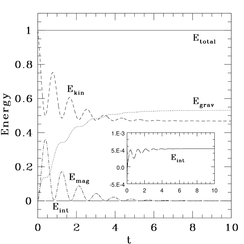
Figure 4.— Energy evolution for Case I ($n=0.001$) with shear viscosity given by $\eta=0.2$. The dotted line labeled “$E_{\rm grav}$” is actually $(E_{\rm grav}-E_{\rm grav}(0))/E_{\rm kin}(0)$. The line labeled “$E_{\rm int}$” is also defined in this way. The expansion of the cylinder causes the gravitational potential energy to become less negative, compensating for the loss of $E_{\rm kin}$. The sum of the energies is conserved and is plotted as the horizontal solid line labeled “$E_{\rm total}$.”

5.2. The ${\mathbf{n}=3}$ Results

We now present results for the slowly differentially rotating $n=3$ case (Case II) without viscosity, and with $\beta=0.030$ ($<\beta_{\rm max}$). The numerical evolution for this model shows a slight overall expansion of the cylinder and radial oscillations which increase in magnitude toward the surface. Oscillations with the same period are also seen in the radial profile of $B_{\phi}$, as shown in Fig. 6, which shows snapshots of the $B_{\phi}$ profile at selected phases of the quasi-oscillation period. This period is $\sim 0.244\,P_{\rm A}$, significantly shorter than the Alfvén period, $P_{\rm A}$, as defined in equation (63). The dynamical timescale for this case, $t_{\rm dyn}=0.0091$ is much shorter than the period of the radial oscillations (since $0.244\,P_{\rm A}=0.400$), and the oscillatory behavior is therefore quasistatic. The angular velocity profiles for this model also display this oscillatory behavior, with the angular velocity becoming more uniform at phases corresponding to maxima in $B_{\phi}$. The radial oscillations show no indication of decaying during the simulation, which ran for several Alfvén timescales: $t_{\rm final}\sim 3\,t_{\rm A}=3.7\,P_{\rm A}$. Thus, with no dissipation mechanism, these oscillations presumably continue indefinitely. [Note, however, that a small amount of viscosity was added in order to stabilize the run, so that $t_{\eta}=70.0\,t_{\rm A}$. This has no significant impact on this run, since the total length of the run was only $\sim 3\,t_{\rm A}$.] That this model does not display any strong radial motions is expected since $\beta=T/|W|$ is below the limit for uniform rotation and hence the configuration can be driven to uniform rotation quasi–periodically without undergoing appreciable contraction and/or expansion.

Figure 5.— Azimuthal magnetic field profiles for Case I with viscosity. The radius $r$ and azimuthal field $B_{\phi}$ are plotted in nondimensional units according to equation (52). Snapshots of the profiles are taken at the same times as in Fig. 3. The behavior is approximately periodic, with a period similar to $P_{\rm A}$. Because of the viscosity, oscillations of the $B_{\phi}$ profile are damped. Note that the profiles do not meet at the radius of the outer mass shell due to the slight expansion of the cylinder.

Now suppose a significant shear viscosity is introduced to the case described in the previous paragraph. As in Case II without viscosity, the cylinder expands slightly. Radial oscillations occur again with roughly the same period ($P\approx 0.244\,P_{A}$), but these oscillations are damped after a few periods due to the shear viscosity. The final state is uniformly rotating with no azimuthal magnetic field. In this case, the cylinder easily relaxes to uniform rotation and dynamical equilibrium within a few oscillation periods of the magnetic field. The excess rotational energy is converted into internal energy (heat).

We now examine the results for the rapidly differentially rotating $n=3$ case (Case III) with $\eta=0$ and $\beta=0.191\gg\beta_{\rm max}$. Though we are interested in the behavior with no shear viscosity, we again add a very small shear viscosity to stabilize the simulation. In this case, taking $\eta$ such that $t_{\eta}=500.0\,t_{\rm A}$ is sufficient, and the effects of the shear viscosity will not be seen in the following results. In all cases discussed hereafter, we will add a similar small, stabilizing viscosity that does not affect the results on the timescales of interest. (This small viscosity will, of course, not be added in cases where we are considering the effects of a significant shear viscosity with $\eta$ chosen such that $t_{\eta}=2.5\,t_{\rm A}$.) The motion of the Lagrangian mass tracers for this case is shown in Fig. 7(a) (Fig. 7(b) shows the analogous results with significant shear viscosity and will be discussed below). The inner $\sim 95\%$ of the mass undergoes a significant contraction and a slight bounce. The inset figure shows that the outer $\sim 5\%$ of the mass expands to large radii, forming a diffuse atmosphere. In the final state, the interior of the star is slowly rotating, having lost most of its angular momentum to the outer envelope.

Figure 6.— Azimuthal magnetic field profiles for Case II ($n~{}=~{}3$ with slow differential rotation) for $\eta=0$. The radius $r$ and azimuthal field $B_{\phi}$ are plotted in nondimensional units according to equation (52). Snapshots of the profiles are taken at steps of $0.061\,P_{A}$. The behavior is seen to be quasi-periodic, with a period of $\sim 0.244\,P_{A}$. For example, the maximum magnitudes of $B_{\phi}$ occur approximately at fractions $1/4,3/4,$ and $5/4$ of the period. This is the same period seen in the gentle radial oscillations which occur during the evolution of this model.

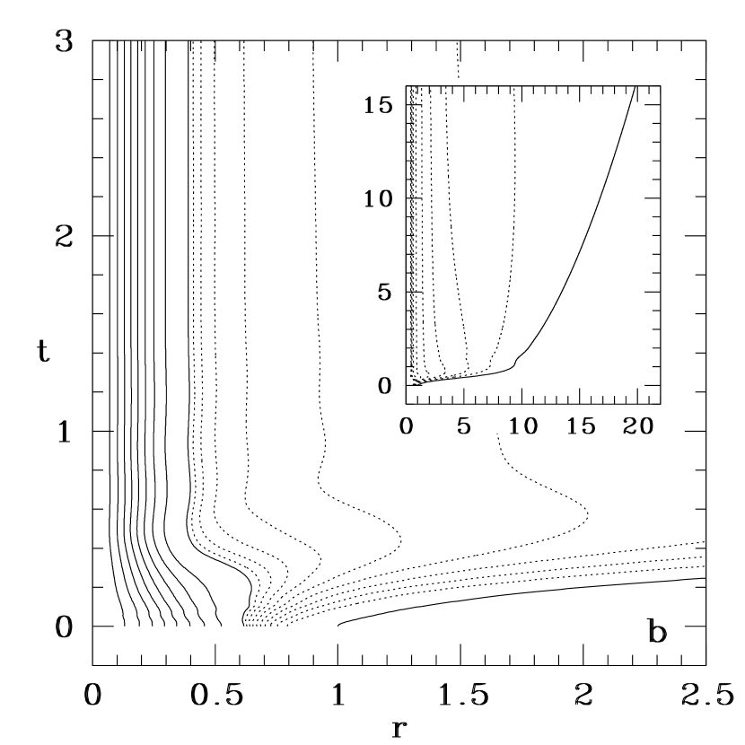
Figure 7.— (a) Spacetime diagram featuring Lagrangian mass tracers for Case III ($n=3$, rapid differential rotation) with $\eta=0$. The solid lines show mass fractions $0.10,0.20,\dots,1.0$ while the dotted lines enclose fractions $0.91,0.92,\dots 0.99$. The large plot demonstrates the contraction of the inner shells and the expansion of the outer envelope. The inset shows the same outermost tracers out to a much larger radius and for a longer time. This inset shows that a diffuse atmosphere has been formed outside of the cylinder. (b) Same as (a) except now with viscosity $\eta=0.2$. The contraction of the inner shells and expansion of the outer envelope shown here are milder than the corresponding behaviors in (a) with zero viscosity.

Figure 7(a) shows that the duration of the contraction is approximately the Alfvén timescale, $t_{\rm A}=2$. The dynamical timescale as defined in equation (59) is much shorter than the Alfvén timescale: $t_{\rm A}=66.4\,t_{\rm dyn}$. Since the contraction takes place over many dynamical timescales, the cylinder is never far from equilibrium and the evolution is quasistatic. The evolution of the virial sum (eq. [64]), which is shown in Fig. 8, illustrates this fact. While the pressure and kinetic energy terms of the virial sum depart significantly from their initial values, the sum $\mathcal{V}$ remains near its equilibrium value of zero. Also, typical radial velocities of the contracting shells have magnitudes only $\sim 10\%$ of the “free-fall velocity,” $\upsilon_{\rm ff}$, where $\upsilon_{\rm ff}\equiv R/t_{\rm dyn}$. In a realistic relativistic hypermassive star, this quasistatic contraction would likely lead to dynamical radial instability and then catastrophic gravitational collapse of the core. The diffuse atmosphere seen in our simulation suggests that magnetic braking operating in rotating stars may also lead to the ejection of winds or a diffuse ambient disk.

Figure 8.— Individual components of the virial sum $\mathcal{V}=(2\Pi+2T+W)/|W|$ for Case III ($\mathcal{V}=0$ in strict equilibrium) with $\eta=0$. The components $2\Pi$, $2T$, and $W$ are normalized to $|W|$ and are plotted with their initial values subtracted off. That $\mathcal{V}$ remains small while the cylinder undergoes significant contraction indicates that the contraction and readjustment occur in a quasistatic fashion.

The time evolution of the various components of the energy is shown in Fig. 9. The most salient feature is the strong contraction, which results in the sharp increase in $E_{\rm int}$ and an increase in the magnitude of the gravitational potential energy. One also sees that, early in the simulation, the magnetic energy grows to an appreciable fraction of the initial rotational kinetic energy. In the final state, most of the kinetic energy has been converted into internal energy by the contraction. Angular momentum is nonetheless conserved because the outer shells are very slowly rotating at very large radii. We show cross-sectional views of the magnetic field lines in Fig. 10. This shows that the maximum magnitude of $B_{\phi}$ occurs early in the run, with some small oscillations following. There is a striking contrast in behavior between this case with rapid differential rotation and Case II discussed above. For Case II, $\beta<\beta_{\rm max}$ and the magnetic field (and viscosity, when present) can drive the cylinder toward uniform rotation without significantly altering the structure of the cylinder. In Case III, however, $\beta$ is significantly larger than $\beta_{\rm max}$ and the cylinder cannot relax to uniform rotation without restructuring. In this case, we see both a strong contraction and expansion of the outer layers. Thus, when the differential rotation is strong, magnetic braking leads to dramatic changes in the stellar structure.

Figure 9.— Energy evolution for Case III ($n=3$ and rapid differential rotation) with $\eta=0$. All energies are defined as in Fig. 4. The rapid rise in $E_{\rm int}$ and sharp drop in $E_{\rm grav}$ correspond to the contraction of the core. The magnetic energy $E_{\rm mag}$ grows to an appreciable fraction of the initial kinetic energy before $B_{\phi}$ decays back to zero in the final state.

Figure 10.— Magnetic field line configurations for Case III ($n=3$, rapid differential rotation) with $\eta=0$ as in Fig. 3. The magnetic field configuration at each time is shown only for the inner $96\%$ of the mass because the outer envelope is ejected to large radius, forming a low-density atmosphere (hence the continuation of each field line outside the cylinder is not shown). The azimuthal magnetic field is clearly strongest at early times.

These results can be compared with the analogous case with significant shear viscosity present ($\eta=0.2$). Figure 7(b) shows the Lagrangian matter tracers for this case. A contraction similar to that seen in Case III with $\eta=0$ is seen again here. However, the inset plot shows that the outer shells are not ejected to such large distances as they are in the previous case. Also, a strong bounce is not seen in the present case. One may conclude that the presence of viscosity has resulted in slightly milder behavior. This is also seen in the fact that the central density increases by a factor of 3.50 in this case, but 3.71 in the case without significant shear viscosity. The approach to uniform rotation in this case is easily seen in Fig. 11, which gives angular velocity profiles at various times. As before, the final state has very little rotational kinetic energy and angular momentum is conserved by transferring angular momentum (via viscosity and magnetic fields in this case) to slowly rotating outer shells at large radii.

Figure 11.— Angular velocity profiles for Case III with $\eta=0.2$ at selected times. The configuration is driven toward slow, uniform rotation. Later profiles extend to $r>1$ because of the expansion of the cylinder. Angular velocity and time are expressed in nondimensional units according to equation (52). Though the final uniform value of $\Omega$ is much smaller than the initial values in the interior, angular momentum is conserved due to the slow rotation of the outer shells at large radii.

The final state for Case III with $\eta=0$ has $\langle P/\rho^{\Gamma}\rangle/\langle P/\rho^{\Gamma}\rangle_{t=0}=1.11$, which indicates that the strong contraction and bounce resulted in significant shock heating. [The symbol $\langle P/\rho^{\Gamma}\rangle$ represents an average of $P/\rho^{\Gamma}$ over the inner 96% of the mass. The average was restricted to the inner 96% because $P/\rho^{\Gamma}$ could not be calculated accurately in the low-density atmosphere.] The existence of shocks is not in conflict with the overall quasistatic nature of the evolution because all of the shocks that we have observed are weak (with Mach numbers in the range $1.0<\mathcal{M}\lesssim 2$) and occur in the outer, low density regions. Consider the shock which formed during this evolution at $t\sim P_{\rm A}/4$ at $\mu(r)/\mu_{t}\sim 0.93$. The MHD shock propagated outward into the atmosphere of the cylinder, and the incoming fluid had a slightly supersonic inward radial velocity with respect to the shock front. The angular velocity and azimuthal magnetic field had discontinuously larger values at the front in the unshocked fluid versus the shocked fluid. This is because the shells falling into the shock front spin up due to momentum conservation. The resulting discontinuity in $\Omega$ then leads to a discontinuity in $B_{\phi}$ due to flux freezing. (In Section 5.4, we will give an example of a shock for which $B_{\phi}$ actually changes sign across the shock front.) We explored the extent to which the quantities upwind and downwind of this shock satisfy the jump conditions for shocks in magnetic fluids (Landau, Lifshitz, & Pitaevskii 1984). For example, the following condition can be derived from continuity of the $z-$ component of the electric field (which applies for a steady state shock) and conservation of mass across the MHD shock front:

$$\rho_{1}\left(\frac{B_{\phi,2}}{\rho_{2}}-\frac{B_{\phi,1}}{\rho_{1}}\right)=\frac{B_{r}}{\upsilon_{r,1}}(\upsilon_{\phi,2}-\upsilon_{\phi,1}),$$ (65)

where the subscripts “1” and “2” refer to the pre- and post-shock fluids respectively (this equation is in physical units, not nondimensional units). The difference between the right and left hand sides of equation (65) for the shock in our numerical solution is $\sim 8\%$. The other jump conditions are also satisfied with errors of $\lesssim 20\%$. This agreement is reasonable considering the simplicity of the artificial viscosity scheme employed by our code and the fact that the jump conditions with which we compared our results assume steady state rather than dynamical conditions.

5.3. The ${\mathbf{n}=1}$ Results

Figure 12.— Density profiles for Case IV ($n=1$) with zero viscosity ($\eta=0$). The radius $r$ and density $\rho$ are plotted in nondimensional units according to equation (52). This plot shows a contraction of the inner material with the outer material forming a diffuse atmosphere.

We now consider the differentially rotating $n=1$ case (Case IV) without viscosity. This case has $\beta=0.168$, which is below the upper limit for uniform rotation, $\beta_{\rm max}$. Recall that all differentially rotating $n=1$ models built according to equation (14) have $\beta<\beta_{\rm max}$. However, $\beta=0.168$ is near the upper limit of $\beta$ for the given rotation law. Even though this case can relax to uniform rotation without appreciable restructuring, we find that this does not happen. The star contracts slightly so that the central density grows by a factor of $1.819$ and sets up a large diffuse atmosphere (see Fig. 12). Figure 13 shows the evolution of the different contributions to the energy. We find that the energy in magnetic fields increases to a significant fraction of the initial kinetic energy, but most of the initial kinetic energy is ultimately converted into internal energy through shock heating. It appears that the final state will be a hot, uniformly rotating star with a dense core and a diffuse atmosphere. We can also see oscillations on the energy plot with a period of $\sim 0.76\,P_{A}$. This is close to the Alfvén period, $P_{\rm A}$, as defined in equation (63). The dynamical timescale for this evolution is $t_{\rm dyn}=0.111$, which is much shorter than the Alfvén time. The virial diagnostic shows that this evolution is quasistatic and similar to the $n=3$ cases. We now consider the effects of adding a shear viscosity. As before, the cylinder develops a large diffuse atmosphere and contracts, but does so slightly less severely than in the case with $\eta=0$. Radial oscillations occur again with roughly the same period ($P\approx 0.76\,P_{A}$), but these oscillations are damped after a few periods due to the shear viscosity. In the $n=1$ inviscid case, the oscillations make determining the final state difficult, but, as can be seen in Fig. 14, the cylindrical model with viscosity tends to uniform rotation by a time $t\sim P_{A}$.

Figure 13.— Energy evolution for Case IV ($n=1$) with $\eta=0$. All energies are defined as in Fig. 4. The sharp increase in $E_{\rm int}$ and sharp decrease in $E_{\rm grav}$ correspond to the contraction of the interior shells. Then as the outer layers continue to expand, $E_{\rm grav}$ increases. Also, $E_{\rm mag}$ grows to an appreciable fraction of the initial kinetic energy before approaching zero. Note the oscillations in the energy components. The sum of the energies is conserved and is plotted as the horizontal solid line.

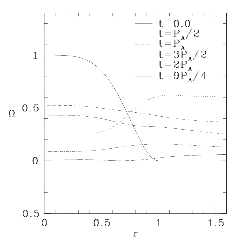
Figure 14.— Angular velocity profiles for Case IV ($n=1$) with $\eta=0.2$. The radius $r$ and angular velocity $\Omega$ are plotted in nondimensional units according to equation (52). Viscosity and magnetic braking drive the star to uniform rotation.

5.4. The ${\mathbf{n}=5}$ Results

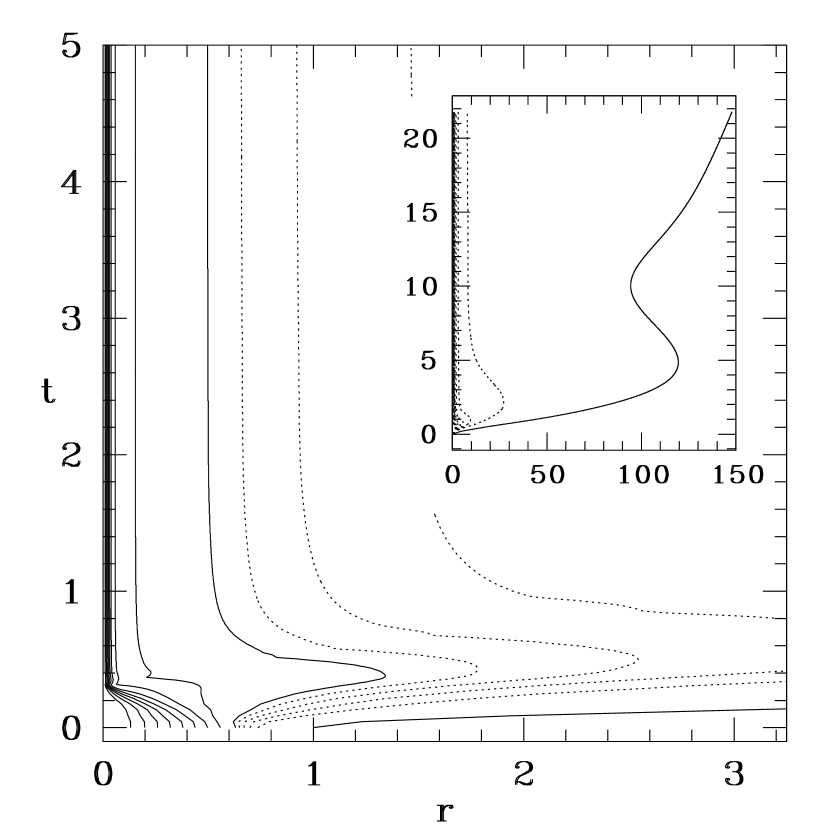
Figure 15.— Spacetime diagram featuring Lagrangian mass tracers for Case VI ($n=5$) without viscosity ($\eta=0.0$). In the large plot, the solid lines enclose mass fractions $0.10,0.20,\dots,1.0$ while the dotted lines enclose fractions $0.92,0.94,0.96$, and $0.98$. In the inset, the solid lines have the same meaning, while the dotted lines enclose fractions $0.91,0.91$ …, $0.99$. The outermost line in the inset encloses a mass fraction of $1.0$. The growth of the azimuthal magnetic field causes a severe contraction of the inner shells and large ejection of the outer layers. The inset shows that the outer layers form a diffuse atmosphere.

We now describe results for the slowly differentially rotating $n=5$ case (Case V) without viscosity. For this case, we choose $\beta=0.0183<\beta_{\rm max}$. Therefore, we do not expect strong radial motions in this case. This case behaves much like the analogous $n=3$ case (Case II), so we do not show any plots for it. The major difference is that this cylinder experienced a slight contraction and radial oscillations which increase in magnitude toward the surface. The central density grows only by a factor of $1.170$ over three Alfvén periods. We also see oscillations in the magnetic field with a period $\sim 0.195\,P_{A}$, much shorter than the Alfvén period. The dynamical timescale for this evolution is $t_{\rm dyn}=0.0020$, which is again much shorter than the Alfvén time. As in the $n=3$ cases, the virial diagnostic shows that this evolution is quasistatic. The only mechanism to dissipate energy is through shock heating, and, since the behavior is mild, this would require a very long run to reach a final state. Adding a significant shear viscosity to this model results in damping of the radial oscillations and rapid approach to uniform rotation, as in Case II.

Figure 16.— Energy evolution for Case VI ($n=5$) with $\eta=0$. All energies are defined as in Fig. 4. The sharp increase in $E_{\rm int}$ and sharp decrease in $E_{\rm grav}$ again correspond to the contraction of the interior shells. Also, $E_{\rm mag}$ grows to an appreciable fraction of the initial kinetic energy before approaching zero.

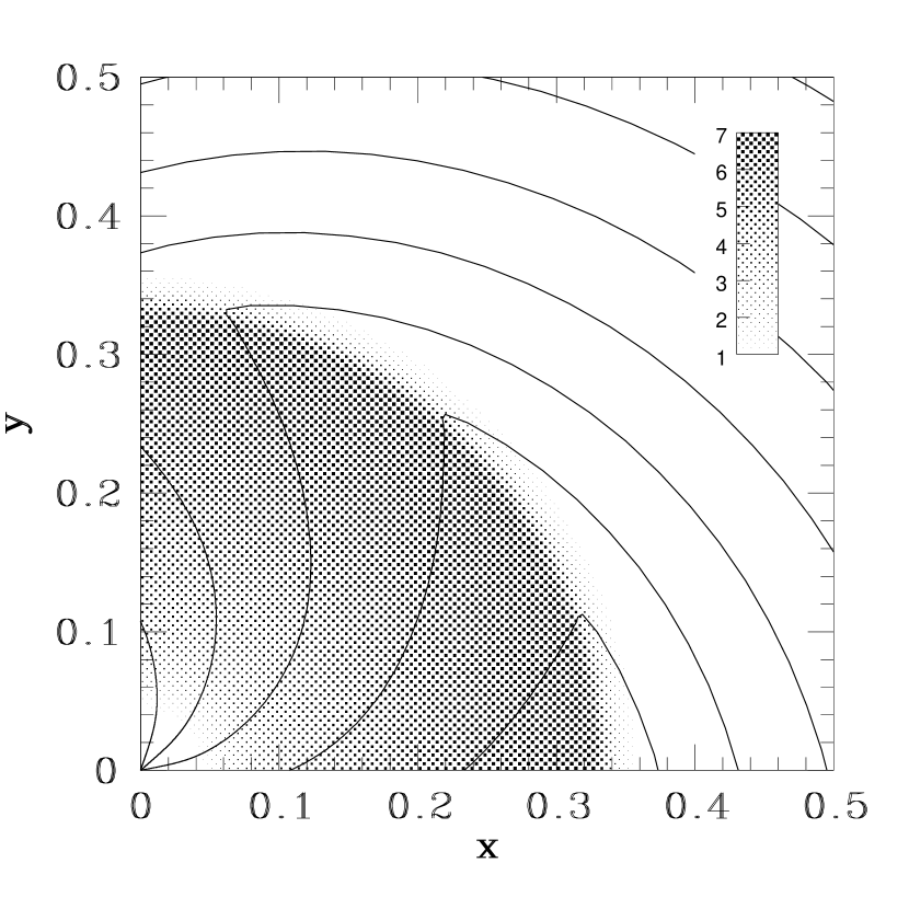
Figure 17.— Outgoing shock for Case VI with $\eta=0$ at time $t=0.24\,P_{\rm A}=0.40$. (Only one quadrant is shown.) The shock front encloses $\sim 83\%$ of the total mass. The ratio $[P/\rho^{\Gamma}]/[P/\rho^{\Gamma}]_{t=0}$ is given by the gray shading, with magnitudes shown in the bar on the upper right. The solid lines are representative magnetic field lines, calculated as in Fig. 3. The discontinuity indicates a change in the sign of $B_{\phi}$.

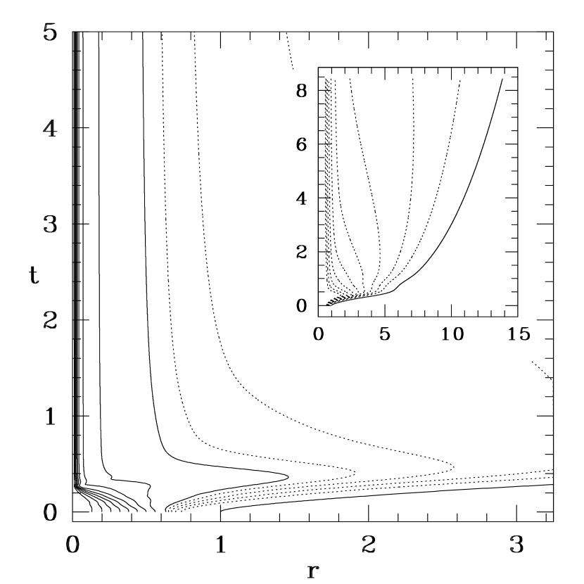
Figure 18.— Spacetime diagram featuring Lagrangian mass tracers for Case VI ($n=5$) with viscosity ($\eta=0.2$). The lines have the same meaning as in Fig. 15. Notice that the contraction is slightly less severe and the ejection much less severe than the case without viscosity.

Next, we examine the results for the rapidly differentially rotating $n=5$ case (Case VI) with $\eta=0$ and where $\beta=0.361\gg\beta_{\rm max}$. The motion of the Lagrangian mass tracers for this case is shown in Fig. 15. The inner $\sim 91\%$ of the mass undergoes a severe contraction. The inset figure shows that the outer $\sim 9\%$ of the mass expands to large radii, forming a diffuse atmosphere. The time evolution of the various components of the energy is shown in Fig. 16, which clearly shows the strong contraction. As in the $n=3$ cases, we see that magnetic braking leads to significant changes in the structure when the rotation is strong. The final state for Case VI with $\eta=0$ has $\langle P/\rho^{\Gamma}\rangle=2.65$, which indicates that the strong contraction resulted in significant shock heating as in Case III. Figure 17 gives a snapshot of an outgoing shock propagating through the envelope in the Case IV evolution. The grayscale shows $[P/\rho^{\Gamma}]/[P/\rho^{\Gamma}]_{t=0}$, a local measure of heating. The solid lines represent magnetic field lines, which are clearly discontinuous at the shock front. However, examining the virial again reveals that this evolution is nearly quasistatic. These results can be compared with the analogous case with significant shear viscosity present ($\eta=0.2$). Figure 18 shows the mass tracers for this case. A contraction similar to that seen in Case VI with $\eta=0$ is seen again here. However, the inset plot shows that the outer shells are not ejected to such large distances as they are in the previous case. Also, the central density increases by a factor of $135.9$ in this case, but $153.39$ in the case without significant shear viscosity. One may conclude that the presence of viscosity has again resulted in slightly milder behavior.

Table 3

Summary of Results

Initial Data Characteristics				Dynamical Behavior	Final State Characteristics
Case	$\beta$	$n$	$\eta$		$\langle P/\rho^{\Gamma}\rangle$	$(R/R_{0})_{50}$	$(R/R_{0})_{90}$	$\rho_{c}/\rho_{c}(0)$
I	0.043	0.001	0.0	standing Alfvén wave	1.00	1.00	1.00	1.00
			0.2	damped oscillations	$\cdots$	1.02	1.08	1.00
II	0.030	3.0	0.0	expansion, oscillations	1.00	0.99	1.00	1.02
			0.2	slight expansion	1.00	0.99	1.00	1.02
III	0.191	3.0	0.0	core contraction	1.11	0.52	0.57	3.71
			0.2	core contraction	1.40	0.53	0.63	3.50
IV	0.168	1.0	0.0	slight contraction	1.07	0.80	0.88	1.82
			0.2	slight contraction	1.22	0.82	0.95	1.77
V	0.018	5.0	0.0	slight contraction, oscillations	1.00	0.92	0.91	1.17
			0.2	slight contraction	1.00	0.92	0.91	1.17
VI	0.361	5.0	0.0	strong core contraction	2.65	0.08	0.78	153.4
			0.2	strong core contraction	2.54	0.09	0.73	135.9

^a $\langle P/\rho^{\Gamma}\rangle$ in units of $\langle P/\rho^{\Gamma}\rangle_{t=0}$; values larger than 1 indicate heating. $(R/R_{0})_{i}$ denotes the radius containing a fraction $i$ of the mass, in units of its initial value.

6. CONCLUSIONS

Poloidal seed magnetic fields and viscosity have important dynamical effects on differentially rotating neutron stars. Even for a small seed magnetic field, differential rotation generates toroidal Alfvén waves which amplify and drive the star toward uniform rotation. This magnetic braking process can remove a significant amount of rotational energy from the star and store it in the azimuthal magnetic field. Though it acts on a longer timescale, shear viscosity also drives the star toward uniform rotation. For a hypermassive star supported against collapse by differential rotation, magnetic braking and viscosity can lead ultimately to catastrophic collapse.

The strength of the differential rotation, the degree of compressibility, and the amount of shear viscosity all affect the response of differentially rotating cylinders to the initial magnetic field. Our calculations have shown very different behavior when $\beta=T/|W|$ is below the upper limit for uniform rotation, $\beta_{\rm max}$, than when it is above this limit. Simulations for $n=3$ and $n=5$ with $\beta<\beta_{\rm max}$ show that the cylinders oscillate and either expand or contract slightly to accommodate the effects of magnetic braking and viscous damping. Large changes in the structure are not seen for these cases. For $\beta>\beta_{\rm max}$, on the other hand, the outer layers are ejected to large radii, while most of the star contracts quasistatically. In a simulation of a relativistic hypermassive star with more realistic geometry, this behavior would likely correspond to quasistatic contraction leading to catastrophic collapse and escape of some ejected material. The dynamical behavior is more extreme for models with greater compressibility. This result is reasonable since softer equations of state allow stronger radial motions. Inclusion of a shear viscosity often moderates the behavior of an evolving model, pacing angular momentum transport and damping the toroidal Alfvén waves which arise due to differential rotation. In particular, the numerical simulations in the rapidly rotating $n=3$ and $n=5$ cases show that the contraction of the core and ejection of the outer shells is milder when a significant shear viscosity is present. Our results are summarized in Table 3.

Though our model for differentially rotating neutron stars is highly idealized, it accommodates magnetic fields, differential rotation, viscosity, and shocks in a simple, one-dimensional Lagrangian MHD scheme. In addition, we are able to handle the wide disparity between the dynamical timescale and the Alfvén and viscous timescales. This disparity will likely prove taxing for relativistic MHD evolution codes since it will be necessary to evolve the system for many dynamical timescales in order to see the effects of the magnetic fields. Because the cylindrical geometry of the present calculation greatly simplifies the computational problem, this class of numerical models is useful in developing intuition for the physical effects which almost certainly play an important role in nascent neutron stars. More realistic evolutionary calculations of magnetic braking in neutron stars will serve to further crystallize our understanding of the evolution of differentially rotating neutron stars, including hypermassive stars that may arise through binary merger or core collapse, and may shed light on the physical origins of gravitational wave sources and gamma ray bursts. Several additional physical effects are expected to be important. For example, Shapiro (Paper I) showed that the presence of an atmosphere outside of the star allows efficient angular momentum loss by partial transmission of Alfvén waves at the surface. This will have important effects on the dynamical behavior of a neutron star relaxing to uniform rotation. In addition, our treatment does not account for evolution of the magnetic field due to turbulence and convection. However, even without these additional physical processes, our calculations reveal qualitatively important features of the effects of magnetic braking on the stability of neutron stars. We hope to continue to pursue these questions through more realistic computational investigations, including the effects of general relativity.

Appendix A THE VIRIAL THEOREM

In this appendix, we closely follow the derivation of the virial theorem in Shapiro & Teukolsky (1983) Section 7.1. We will discuss the inviscid case, because we do not expect viscosity to play a dominant role in equilibrium stars. We start by dotting the position vector $\mathbf{x}$ into equation (31). We then multiply through by $\rho$, integrate over a cylindrical volume of length $L$ and radius $R$, and divide by $L$ (we will work with quantities per unit length as we did in section 3.3). Define $T$, $\Pi$, and $W$ as in section 3.3 and the moment of inertia per unit length as

$$I\equiv\int_{0}^{R}\rho r^{2}d\mathcal{A}.$$ (A1)

The left hand side of equation (31) then becomes

$$\frac{1}{2}\frac{d^{2}I}{dt^{2}}-2T.$$ (A2)

The gravitational term is $W$. We will calculate the pressure term in detail to display a feature of this geometry. The pressure term is

$$-\frac{1}{L}\int\mathbf{x}\cdot\mathbf{\nabla}Pd^{3}x = -\frac{1}{L}\int\mathbf{\nabla}\cdot(P\mathbf{x})d^{3}x+\frac{1}{L}\int P\mathbf{\nabla}\cdot(\mathbf{x})d^{3}x$$ (A3)

$$= -\Pi+3\Pi,$$

where we have used

$$-\frac{1}{L}\int\mathbf{\nabla}\cdot(P\mathbf{x})d^{3}x = -\frac{1}{L}\oint P\mathbf{x}\cdot\hat{\mathbf{n}}d\mathcal{A}$$ (A4)

$$= -\Pi.$$

The difference between this infinite cylinder case and the case for bounded distributions is that we must keep a term from the endcaps when applying the divergence theorem in equation (A4). Applying similar manipulations to the magnetic terms shows that these terms cancel. Collecting these results gives

$$\frac{1}{2}\frac{d^{2}I}{dt^{2}}=2T+W+2\Pi.$$ (A5)

Assuming steady-state ($d/dt=0$) gives the virial theorem quoted in equation (17).

Appendix B STABILITY OF CYLINDRICAL POLYTROPES

In this section, we derive by means of an energy variational calculation the critical polytropic parameter $\Gamma_{\rm crit}$ for the stability of a slowly rotating cylinder against radial perturbations, adapting the treatment of stability for ordinary stars given in Shapiro and Teukolsky (1983). Because we are considering equilibrium models, there is no azimuthal magnetic field, and we can take the total energy as

$$E=E_{\rm int}+T+E_{\rm grav},$$ (B1)

where $T$ is the rotational kinetic energy. Consider a sequence of rotating equilibrium cylinders with constant angular momentum per unit length, $J$, parameterized by central density, $\rho_{c}$. The equilibrium mass per unit length $\mu_{t}$ is determined by the condition $\partial E/\partial\rho_{c}=0$. Stability then requires $\partial^{2}E/\partial\rho_{c}^{2}\geq 0$. Using the $\Gamma$-law EOS for polytropes,

$$E_{\rm int}=\int d\mu\frac{K\rho^{\Gamma-1}}{\Gamma-1}=k_{1}K\mu_{t}\rho_{c}^{\Gamma-1},$$ (B2)

where $k_{1}$ is some nondimensional constant of order unity that depends on the density profile through $\Gamma$ for slowly rotating configurations. The kinetic energy is just $T=J^{2}/2I$, where $I$ is the moment of inertia per unit length. Since $I\propto\mu_{t}R^{2}\propto\mu_{t}^{2}/\rho_{c}$, one may write

$$T=k_{2}\frac{J^{2}\rho_{c}}{\mu_{t}^{2}},$$ (B3)

where $k_{2}$ is another constant. (We note that $k_{1}$ and $k_{2}$ may be derived analytically for nonrotating cylinders by rewriting the integral in terms of Lane-Emden variables.)

Next consider the gravitational potential energy. As in equation (4.2), the gravitational energy per unit length is

$$E_{\rm grav}=\text@frac{1}{2}\int dr2\pi r\rho\Phi=\text@frac{1}{2}\int_{0}^{R}dr\frac{\partial\mu}{\partial r}\Phi.$$ (B4)

Now from equation (5), $\partial\Phi/\partial r=2\mu(r)/r$. Integrating this equation inward from a fiducial radius $r_{0}$ outside of the cylinder gives

$$\Phi(r)=2\mu_{t}\ln(r/r_{0}),\,\,\,\,\,(r\geq R).$$ (B5)

We now integrate the right-hand side of equation (B4) by parts, insert the forms for $\Phi$ and its radial derivative, and obtain

$$E_{\rm grav}=\mu_{t}^{2}\ln(R/r_{0})-\int dr\frac{\mu^{2}(r)}{r}.$$ (B6)

Any terms independent of $\rho_{c}$ may be discarded for the purposes of this variational calculation. The second term on the r.  h.  s.  of equation (B6) scales as $\mu_{t}^{2}$ and is independent of $\rho_{c}$. However, the first term depends on $\rho_{c}$ since $R^{2}\propto\mu_{t}/\rho_{c}$. Then

$$E_{\rm grav}=\text@frac{1}{2}\mu_{t}^{2}\ln\left(\frac{\mu_{t}}{\rho_{c}r_{0}^{2}}\right)+{\rm constants}.$$ (B7)

From equations (B2), (B3), and (B7), the total energy is (up to additive constants)

$$E=k_{1}\mu_{t}K\rho_{c}^{\Gamma-1}+k_{2}\frac{J^{2}\rho_{c}}{\mu_{t}^{2}}+\text@frac{1}{2}\mu_{t}^{2}\ln\left(\frac{\mu_{t}}{\rho_{c}r_{0}^{2}}\right).$$ (B8)

The conditions for equilibrium and for the onset of instability become

$$\frac{\partial E}{\partial\rho_{c}}= 0 =k_{1}(\Gamma-1)\mu_{t}K\rho_{c}^{\Gamma-2}+k_{2}\frac{J^{2}}{\mu_{t}^{2}}-\frac{\mu_{t}^{2}}{2\rho_{c}}$$

$$\frac{\partial^{2}E}{\partial\rho_{c}^{2}}= 0 =k_{1}(\Gamma-1)(\Gamma-2)\mu_{t}K\rho_{c}^{\Gamma-3}+\frac{\mu_{t}^{2}}{2\rho_{c}^{2}}.$$ (B9)

The first equation is equivalent to the condition for hydrostatic equilibrium (see eq. [10]). Inserting the first equation into the second to eliminate the term proportional to $k_{1}$ gives, after rearranging,

$$\text@frac{1}{2}(\Gamma-1)-(\Gamma-2)\frac{k_{2}J^{2}\rho_{c}}{\mu_{t}^{2}}\frac{1}{\mu_{t}^{2}}=0.$$ (B10)

Now, by equation (18), $\mu_{t}^{2}=|W|$, where $W$ is the gravitational term appearing in the virial theorem. We also use equation (B3) to identify the kinetic energy $T$. Since equation (B10) is the condition marking the onset of instability, solving for $\Gamma$ gives the critical value:

$$\Gamma_{\rm crit}=\frac{(1-4T/|W|)}{(1-2T/|W|)}\;\;\;\;({\rm cylinders}).$$ (B11)

By contrast, the result for ordinary bounded stars is (Shapiro & Teukolsky 1983)

$$\Gamma_{\rm crit}=\frac{4}{3}\frac{(1-5T/2|W|)}{(1-2T/|W|)}\;\;\;\;({\rm bounded~{}stars}).$$ (B12)

Note that, for nonrotating cylinders with $T/|W|=0$, the critical polytropic parameter is $\Gamma_{\rm crit}=1$. For larger values of $T/|W|$, $\Gamma_{\rm crit}$ decreases. But since $\Gamma=1$ is the smallest $\Gamma$ obtainable for any positive polytropic index $n$, all equilibrium cylindrical polytropes are radially stable.

Appendix C NUMERICAL TECHNIQUES

We solve the MHD evolution equations using a one-dimensional Lagrangian finite differencing scheme in which the cylinder is partitioned in the radial direction into $N$ shells of equal mass per unit length. The evolution equations are differenced on staggered meshes in time and space. The quantities $r$, $\upsilon_{r}$, $j$, and $\mu$ are defined on the shell boundaries while $P$, $V\equiv 1/\rho$, $\varepsilon$, $B_{\phi}$, and $q$, the artificial viscosity, are defined at the shell centers. Integral and half-integral spatial indices correspond to shell boundaries and shell centers, respectively. For example, one has $r_{i}$ where $i=1,2,\dots,N+1$ and $P_{i+1/2}$ where $i=1,2,\dots,N$. Updating at each timestep occurs in leap-frog fashion, with $\upsilon_{r}$, $q$, and $j$ defined at times with half-integral indices ($t^{n+1/2}$) and $r$, $P$, $V$, $B_{\phi}$, and $\varepsilon$ defined at times $t^{n}$.

Shocks are handled using artificial viscosity as described by Richtmyer and Morton (1967). In physical units, the artificial viscosity prescription is

$$q=\cases{\frac{(a\delta r)^{2}}{V}\left(\frac{\partial\upsilon_{r}}{\partial r}\right)^{2},&if $\partial\upsilon_{r}/\partial r<0$;\cr 0,&otherwise.\cr}$$ (C1)

where $\delta r$ is the typical spatial mesh size and the thickness of the resulting smoothed shock is approximately $a^{2}\delta r$ (we usually take $a=1.75$). The timestep is governed by the usual Courant condition in the absence of viscosity: $\delta t=b\delta r/c_{s}$, where $c_{s}$ is the local sound speed and $b$ is an constant less than unity (we usually take $b=0.3$). If shear viscosity is present, the condition becomes

$$\delta t={\rm min}\left\{b\frac{\delta r}{c_{s}},b\frac{(\delta r)^{2}}{2D_{\rm eff}}\right\},$$ (C2)

where $D_{\rm eff}=4\eta/3\rho$ is an effective diffusion coefficient.

We found it convenient to use a different nondimensionalization scheme for our numerical scheme than was employed in the discussion above (eq.  [52]). We will now use the following definitions:

$$\tilde{r}=r/R,\;\;\;\tilde{t}=t/(R/c_{s}(0)),\;\;\;\tilde{\eta}=\eta/(\rho_{c}c_{s}(0)R),$$

$$\tilde{j}=j/(c_{s}(0)R),\;\;\;\tilde{B}_{\phi}=B_{\phi}/B_{0},$$

$$\tilde{\rho}=\rho/\rho_{c},\;\;\;\tilde{\upsilon}_{r}=\upsilon_{r}/c_{s}(0),\;\;\;\tilde{\varepsilon}=\varepsilon/[K\rho_{c}^{\Gamma-1}/(\Gamma-1)]$$

$$\tilde{\mu}=\mu/(\rho_{c}R^{2}),\;\;\;\tilde{P}=P/(K\rho_{c}^{\Gamma}),$$

where $c_{s}(0)=(\Gamma K\rho_{c}^{\Gamma-1})^{1/2}$ is the sound speed at $r=0$ and $t=0$. This differs from the previous scheme in that it relies on the sound speed as a velocity scale rather than the Alfvén speed. We finite-difference the evolution equations (39)-(42), using equations (C) to write the system in nondimensional form. (Below we drop the tildes on all nondimensional quantities.) If no shear viscosity is present, all derivatives are approximated by second order centered differences, so that the scheme is second order in space and time (except at the boundaries). The terms which account for shear viscosity are not time centered (i.e. these terms are first order in time). This simplification does not significantly affect our results since the viscous terms are small compared to the other terms in the evolution equations.

Before giving the evolution system, we will introduce several definitions and conventions to simplify the notation. First, we will drop the $r$ index on $\upsilon_{r}$, the $\phi$ index on $B_{\phi}$, and the tildes. We also define $\theta\equiv\upsilon_{\rm A}/c_{s}(0)$. In all of the following equations, the operator $\Delta$, which takes a spatial difference, will be defined by $\Delta Q_{i}=Q_{i}-Q_{i-1}$. In some of the equations, it is useful to define space and time averages for grid positions with half-integral indices. For example, $r_{i+1/2}^{n}\equiv(r_{i+1}^{n}+r_{i}^{n})/2$ and $r_{i}^{n+1/2}\equiv(r_{i}^{n+1}+r_{i}^{n})/2$. Then the evolution equation for specific angular momentum (eq. [40]) becomes

$$\frac{j_{i}^{n+1/2}-j_{i}^{n-1/2}}{\delta t}=\frac{2\pi\theta^{2}}{\delta\mu}\Delta(r_{i+1/2}^{n}B_{i+1/2}^{n})+\frac{2\pi\eta}{\delta\mu}\Delta\left[\frac{1}{2}\left(\frac{(r_{i+1}^{n})^{3}+(r_{i}^{n})^{3}}{\Delta r_{i+1}^{n}}\right)\Delta\left(\frac{j_{i+1}^{n-1/2}}{(r_{i+1}^{n})^{2}}\right)\right].$$ (C4)

We have used the fact that the Lagrangian mass increment between two shells, $\delta\mu$ is a constant. The radial velocity is updated next as follows:

$$\frac{\upsilon_{i}^{n+1/2}-\upsilon_{i}^{n-1/2}}{\delta t} = -\frac{2\pi r_{i}^{n}}{\Gamma\delta\mu}\Delta(P_{i+1/2}^{n})-\left(\frac{n\xi_{1}^{2}}{2\pi}\right)\frac{\mu_{i}}{r_{i}^{n}}-\frac{\pi\theta^{2}}{\delta\mu r_{i}^{n}}\Delta((r_{i+1/2}^{n})^{2}B_{i+1/2}^{n})$$ (C5)

$$+\frac{1}{2(r_{i}^{n})^{3}}[(j_{i}^{n+1/2})^{2}+(j_{i}^{n-1/2})^{2}]$$

$$+\frac{8\pi\eta}{3\delta\mu r_{i}^{n}}\Delta\left[\frac{1}{2}\left(\frac{(r_{i+1}^{n})^{3}+(r_{i}^{n})^{3}}{\Delta r_{i+1}^{n}}\right)\Delta\left(\frac{\upsilon_{i+1}^{n-1/2}}{r_{i+1}^{n}}\right)\right].$$

The $\xi_{1}$ appearing in the gravitational potential term of the above equation is just the nondimensional surface radius from the solution of the Lane-Emden equation. It arises here only because of our choice of nondimensionalization. Next, we update the locations of shell boundaries according to

$$\frac{r_{i}^{n+1}-r_{i}^{n}}{\delta t}=\upsilon_{i}^{n+1/2}.$$ (C6)

The specific volume of each shell is then updated to reflect the new shell boundaries:

$$V_{i+1/2}^{n+1}=V_{i+1/2}^{0}\left(\frac{\Delta(r_{i+1}^{n+1})^{2}}{\Delta(r_{i+1}^{0})^{2}}\right),$$ (C7)

where the superscript “0” refers to the initial value (this equation merely expresses the fact that the volume of a thin shell is $dV=\pi Ldr^{2}$). We next integrate the evolution equation for the magnetic field.

$$\frac{B_{i+1/2}^{n+1}-B_{i+1/2}^{n}}{\delta t}=-\frac{1}{2}(B_{i+1/2}^{n+1}+B_{i+1/2}^{n})\left(\frac{\Delta\upsilon_{i+1}^{n+1/2}}{\Delta r_{i+1}^{n+1/2}}\right)+\frac{1}{\Delta r_{i+1}^{n+1/2}}\Delta\left(\frac{j_{i+1}^{n+1/2}}{(r_{i+1}^{n+1/2})^{2}}\right).$$ (C8)

This equation can be solved for the updated magnetic field in each cell, $B_{i+1/2}^{n+1}$. The next quantity to update is the artificial viscosity:

$$q_{i+1/2}^{n+1/2}=\cases{\frac{2a^{2}\Gamma}{V_{i+1/2}^{n+1/2}}(\Delta\upsilon_{i+1}^{n+1/2})^{2},&if $\Delta\upsilon_{i+1}^{n+1}<0$;\cr 0,&otherwise.\cr}$$ (C9)

The specific internal energy is updated according to the First Law of Thermodynamics with entropy generation terms due to the presence of viscosity (see eq. [57]):

$$\frac{\varepsilon_{i+1/2}^{n+1}-\varepsilon_{i+1/2}^{n}}{\delta t}=-\frac{1}{2n}(P_{i+1/2}^{n+1}+P_{i+1/2}^{n})\left(\frac{V_{i+1/2}^{n+1}-V_{i+1/2}^{n}}{\delta t}\right)+\frac{\Gamma\eta}{n}V_{j+1/2}^{n+1/2}f_{j+1/2}^{n+1/2}(\upsilon,j,r),$$ (C10)

where

$$f_{i+1/2}^{n+1/2}(\upsilon,j,r) \equiv \frac{2}{9}\left[\left\{2\frac{\Delta\upsilon_{i+1}^{n+1/2}}{\Delta r_{i+1}^{n}}-\frac{\upsilon_{i+1/2}^{n+1/2}}{r_{i+1/2}^{n}}\right\}^{2}+\left\{\frac{(r_{i+1}^{n})^{2}+(r_{i}^{n})^{2}}{2\Delta r_{i+1}^{n}}\Delta\left(\frac{\upsilon_{i+1}^{n+1/2}}{(r_{i+1}^{n})^{2}}\right)\right\}^{2}\right.$$ (C11)

$$+\left.\left\{2\frac{\Delta(r_{i+1}^{n}\upsilon_{i+1}^{n+1/2})}{\Delta(r_{i+1}^{n})^{2}}\right\}^{2}\right]+\left\{\frac{r_{i+1/2}^{n}}{\Delta r_{i+1}^{n}}\Delta\left(\frac{j_{i+1}^{n+1/2}}{(r_{i+1}^{n})^{2}}\right)\right\}^{2}.$$

Note that the terms due to viscous dissipation are not time-centered. Equation (C10) may be solved for the updated value of the specific internal energy, $\varepsilon_{i+1/2}^{n+1}$, by first substituting for the (as yet unknown) updated pressure, $P_{i+1/2}^{n+1}$, according to the $\Gamma$-law EOS:

$$P_{i+1/2}^{n+1}=\varepsilon_{i+1/2}^{n+1}/V_{i+1/2}^{n+1}.$$ (C12)

Finally, the pressure itself is updated using equation (C12). In order to evolve the system from one timestep to the next, equations (C4)-(C12) are used in the order as given above to updated each quantity. These equations only apply in the interior regions of the grid and some must be modified to accommodate boundary conditions on the cylinder axis ($r=0$) and at the surface. These modifications result in only first order spatial accuracy near these boundaries.

All of the calculations described in this paper were performed on single processors and none lasted more than a few hours. As an example, consider the rapidly rotating $n=3$ cylinder with $\eta=0$. This run required 2400 Lagrangian mass shells and each timestep required 7.295 ms of CPU time on a Pentium IV, 2.0 GHz processor. The total length of this run was $4.4\times 10^{6}$ steps. Our runs required spatial resolution in the range of 400-2400 Lagrangian mass shells.

References

- (1) Andersson, N. 1998, ApJ, 502, 708
- (2) Andersson, N., Kokkotas, K. D., & Stergioulas, N. 1999, ApJ, 516, 307
- (3) Baumgarte, T. W., & Shapiro, S. L. 1999, ApJ, 526, 941
- (4) Baumgarte, T. W., & Shapiro, S. L. 2003, ApJ, 585, 921
- (5) Baumgarte, T. W., & Shapiro, S. L., & Shibata, M. 2000, ApJ, 528, L29
- (6) Bromm, V., & Loeb, A. 2003, ApJ, 596, 34 (astro-ph/0212400)
- (7) Chandrasekhar, S. 1939, An Introduction to the Study of Stellar Structure, (Chicago: Univ. Chicago Press)
- (8) Coburn, W. & Boggs, S. E. 2003, Nature, 423, 415
- (9) Cutler, C., & Lindblom, L. 1987, ApJ, 314, 234
- (10) Friedman, J. L., & Morsink, S. 1998, ApJ, 502, 714
- (11) Landau, L. D., & Lifshitz, E. M. 1998, Fluid Mechanics, (Oxford: Butterworth-Heinemann)
- (12) Landau, L. D., Lifshitz, E. M., & Pitaevskii, L. P. 2000, Electrodynamics of Continuous Media, (Oxford: Butterworth-Heinemann)
- (13) Lindblom, L., Owen, B. J., & Morsink S. 1998, Phys. Rev. Lett., 80, 4843
- (14) Liu, Y. T., & Lindblom, L. 2001, MNRAS, 342, 1063
- (15) Liu, Y. T. 2002, Phys. Rev. D, 65, 124003
- (16) MacFadyen, A., & Woosley, S. E. 1999, ApJ, 524, 262
- (17) Meszaros, P., & Rees, M. J. 1997, ApJ, 482, L29
- (18) Narayan, R., Paczynski, B., & Piran, T. 1992, ApJ, 395, L83
- (19) Piran, T. 2002, in Proceedings of GR16 (Singapore: World Scientific), in press (gr-qc/0205045)
- (20) Rampp, M., Müller, E., & Ruffert, M. 1998, A&A, 332, 969
- (21) Rasio, F. A., & Shapiro, S. L. 1992, ApJ, 401, 226
- (22) Rasio, F. A., & Shapiro, S. L. 1999, Class. Quant. Grav., 16, R1
- (23) Rees, M. J. 1984, ARA&A, 22, 471
- (24) Rezzolla, L., Lamb, F., Marcović, D., & Shapiro, S. L. 2001a, Phys. Rev. D, 64, 104013
- (25) Rezzolla, L., Lamb, F., Marcović, D., & Shapiro, S. L. 2001b, Phys. Rev. D, 64, 104014
- (26) Rezzolla, L., Lamb, F., & Shapiro, S. L. 2000, ApJ, 531, L141
- (27) Richtmyer, R. D., & Morton, K. W. 1967, Difference Methods for Initial Value Problems (New York: Wiley)
- (28) Ruffert, M., & Janka, H.-T. 1999, A&A, 344, 573
- (29) Sari, R., Piran, T., & Halpern, J. P. 1999, ApJ, 519, L17
- (30) Sawyer, R. F. 1989, Phys. Rev. D, 39, 3804
- (31) Shapiro, S. L. 1980, ApJ, 240, 246
- (32) Shapiro, S. L. 2000, ApJ, 544, 397 (Paper I)
- (33) Shapiro, S. L. 2003, in Carnegie Observatories Astrophysics Ser. 1, Coevolution of Black Holes and Galaxies, ed. L. C. Ho (Cambridge: Cambridge Univ. Press), in press (astro-ph/0304202)
- (34) Shapiro, S. L., & Teukolsky, S. A. 1983, Black Holes, White Dwarfs, and Neutron Stars, (New York: Wiley)
- (35) Shibata, M., & Uryū, K. 2000, Phys. Rev. D, 61, 064001
- (36) Tassoul, J. L. 1978, Theory of Rotating Stars (Princeton: Princeton Univ. Press)
- (37) Vlahakis, N., & Konigl, A. 2001, ApJ, 563, L129
- (38) Zwerger, T., & Müller, E. 1997, A&A, 320, 209