Asymfast,
a method for convolving maps with asymmetric main beams

Abstract

We describe a fast and accurate method to perform the convolution of a sky map with a general asymmetric main beam along any given scanning strategy. The method is based on the decomposition of the beam as a sum of circular functions, here Gaussians. It can be easily implemented and is much faster than pixel-by-pixel convolution. In addition, Asymfast can be used to estimate the effective circularized beam transfer functions of CMB instruments with non-symmetric main beam. This is shown using realistic simulations and by comparison to analytical approximations which are available for Gaussian elliptical beams. Finally, the application of this technique to Archeops data is also described. Although developped within the framework of Cosmic Microwave Background observations, our method can be applied to other areas of astrophysics.

I Introduction

With the increasing in accuracy and angular scale coverage of the recent Cosmic Microwave Background (CMB) experiments, a major objective is to include beam uncertainties when estimating cosmological parameters bridle , and in particular the asymmetry of the beam arnau . As seen in Cosmosomas cosmosomas , Boomerang boom , Maxima maxima , Archeops archeops , WMAP wmap and anticipated for Planck, the systematics errors are dominated at the smaller scales (higher multipoles, $\ell$) by the uncertainties on the reconstruction of and deconvolution from the beam pattern. So the beam must be considered more realistically, in particular by rejecting the assumptions of Gaussianity and/or symmetry. It leads to a better modelization of the beam to convolve with and a better estimation of its representation in the harmonic space, its transfer function $B_{\ell}^{eff}$.

The use of simulated sky maps takes an important part in the analysis of astrophysical data sets to study possible systematic effects and noise contributions, and also, to compare the data to theoretical predictions or to observations from other instrumental setups. This is one of the most challenging problems in data analysis : obtaining a simple and accurate model for the instrumental response. In many cases, Monte-Carlo approaches are favoured as they are in general simpler than the analytic ones. However, they need a great number of simulations which often requires too much time of execution for the available computing facilities. A large amount of this time is spent in the convolution of the simulated data by the instrumental response or beam pattern. For an asymmetric beam, the convolved map at a given pointing direction on the sky would depend both on the relative orientation of the beam on the sky and on the shape of the beam pattern. This makes brute-force convolution particularly painful and slow (e.g. buriganaLFI ).

Therefore, either we work in the spherical harmonic space using a general and accurate convolution algorithm (see wandelt for a fast implementation), either we model the beam pattern by a series of easy-to-deal-with functions and compute for each a fast convolution in the harmonic space.

The work of wandelt presents how to convolve exactly two band limited but otherwise arbitrary functions on the sphere - which can be the 4-$\pi$ beam pattern and the sky descriptions. At each point on the sphere, one computes a ring of different convolution results corresponding to all relative orientations about this direction. To allow subsequent interpolation at arbitrary locations it is sufficient to discretize each Euler angle describing the position on the sphere into ${{\cal O}\!\left(L\right)}$ points where L measures the larger of the inverse of the smallest length scale of the sky or beam. The method rapidity depends on the scanning strategy : in ${{\cal O}\!\left(L^{3}\right)}$ for constant-latitude scans and in ${{\cal O}\!\left(L^{4}\right)}$ for other strategy - even if factorization may be found in some cases. This method is used for Planck simulations in case of elliptical Gaussian beams for the polarized channels whansen and is one of the most promising techniques to decrease side-lobe effects on the WMAP results barnes . While it is efficient for a certain class of observational strategies whansen , it may be difficult to implement in the more general case of non-constant latitude scanning strategies challinor .

For the second method based on the modelling the beam pattern, several solutions have been proposed either circularizing the beam (page or wu ) or assuming an elliptical Gaussian beam (souradeep or pablo ). Here we propose an alternative method, Asymfast, which easily can account for any main beam shape. In general the main beam maps can be obtained from point-sources like the planets Jupiter and Saturn (see chiang for a general view, beamplanck , beamlfi for HFI, LFI beams and page for WMAP beams). The beam maps are then fitted with the appropriate model from which the beam transfer function can be computed. Moreover the beam modelization can be used as input for deconvolution methods like burigana or optimal map-making iterative methods as MapCUMBA dore .

By contrast to wandelt , Asymfast deals only with main beams which are decomposed onto a sum of 2D symmetric Gaussians and does not take into account far-side lobes. In the following, we will simply call Gaussian a 2D symmetric Gaussian function. The sky is then easily convolved by each Gaussian and the resulting convolved sub-maps are combined into a single map which is equivalent to the sky convolved by the asymmetric original beam. This method can be used for any observational strategy and is easy to implement. As the goal of Asymfast is only to deal with main beams, we shall not directly compare with the wandelt method in this paper.

The use of 4-$\pi$ beam is beyond the scope of Asymfast and so Asymfast and the wandelt method are not directly compared in this paper.

We describe our approach in Section II and the simulations we used to check the accuracy and performance of the method in Section III. Section IV describes the symmetric expansion of the beam. In Section V, we compare the accuracy of our method with respect to the elliptical Gaussian and the brute-force approach. Section VI discusses the time-computing efficiency of the different convolution method considered. Finally, in Section VII, we describe a method to estimate the effective beam transfer function. This technique has been successfully used for the determination of the Archeops main beam in section VIII.

II Method

Asymfast approaches any asymmetric beam by a linear combination of Gaussian functions centered at different locations within the original beam pattern.

The convolution is performed separetly for each Gaussian and then the convolved maps are combined into a single map. The map convolution with the Gaussian beams is computed in the spherical harmonic space. This allows us to perform the convolution in a particularly low time consuming way. By contrast, the brute-force convolution by an asymmetric beam needs to be performed in the real space for each of the time samples so that the relative orientation of the beam on the sky is properly taken into account for each pointing direction.

The Asymfast method can be described in five main steps :

1. The beam is decomposed into a weighted sum of $N$ Gaussians. The number of Gaussians is chosen by minimazing residuals according to user-defined precision (see Section IV).

2. The initial map is oversampled by a factor of 2 and convolved with each of the Gaussian functions. The sky map is decomposed into $a_{\ell m}$ coefficients in the harmonic space. Then, $N$ sub-maps are computed, each of them smoothed with the corresponding Gaussian sub-beam, by multiplying the $a_{\ell m}$ coefficients of the original sky map by the current approximation of the transfer functions of the Gaussian beams $B_{\ell}^{N}=\exp\left[-\ell\left(\ell+1\right)\sigma_{N}^{2}\right]$.

3. The sub-maps are deprojected into timelines using the scanning strategy of the corresponding sub-beam position.

4. The $N$ timelines are stacked into a single one weighted by their sub-beam amplitude.

5. The timeline obtained this way is projected onto the sky with the scanning strategy corresponding to the center of the beam pattern and we obtain the convolution of the original sky map with the fitted beam along the scan.

The HEALPix healpix package is used to store maps (ring description), to compute the decomposition of the sky map in spherical harmonics (anafast) and to reconstruct maps from the $a_{\ell m}$ coefficients (synfast).

III Beams and scanning strategy simulations

The method was checked using realistic simulations of a sky observation performed by an instrument with asymmetric beam pattern and complex scanning strategy. To keep the time consumption reasonnable within our computing capabilities without degrading the quality of the results, we have chosen beams with FWHM between 40 and 60 arcmin sampled by steps of 4 arcmin (square beam map of 60$\times$60 pixels corresponding to 4$\times$4 deg).

We consider two sets of simulations : a first one corresponding to a quasi-circular beam to which we have added 1 % (simulation 1a) and 10 % (simulation 1b) of noise, and a second one corresponding to an irregular beam to which we have also added noise in the same way (simulations 2a and 2b). These two sets are obtained from a sum of a random number of elliptical Gaussians with random positions within 0.4 degree around the center and random FWHMs and amplitudes. Then, the beams are smoothed with a 4 arcmin width Gaussian and white noise is added.

The scanning strategy is assumed to be a set of consecutive meridians with sampling of 3 arcmin over each meridian and a lag of 3 arcmin between two meridians. This strategy is roughly similar to the Planck observing plan. It allows an efficient check of the method as, close to the equator, all beams are parallel and the effect of the orientation is maximum. However, close to the pole, the high number of beams in different direction per pixel makes the effective beam more circular. In order to save time, we keep only half an hemisphere of the sky, so we use about 6.5 million data samples. The number of hits per pixel is highly variable from equator to pole, ranging from 1 to about 8000 near the pole.

For high-resolution instruments, like Planck, we should consider maps with resolution of the order of 1 arcmin. However, this would require too much computing time for brute-force convolution. Instead, in this paper, we consider maps of the sky with pixel size of $\approx$24 arcmin which are stored in the HEALPix format ($N_{side}=256$). We have checked that the results obtained with Asymfast considering lower resolution maps with larger beams can be generalized to higher resolution maps with narrower beams.

IV Symmetric Gaussian expansion of the beam

We model the original beam pattern using $N$ Gaussians, $i\in\{1,N\}$, of the form

$$g(x_{i},y_{i},\sigma_{i};x,y)=\frac{1}{2\pi\sigma_{i}^{2}}\exp\left[\frac{(x-x_{i})^{2}+(y-y_{i})^{2}}{2\sigma_{i}^{2}}\right]$$ (1)

The beam is fitted with a weighted sum of the $N$ Gaussians :

$$b(x,y)=\sum_{i=1}^{N}A_{i}g(x_{i},y_{i},\sigma_{i};x,y)$$ (2)

so we have $4N$ free parameters corresponding to width ($\sigma_{i}$, FWHM = $\sqrt{8ln2}\sigma_{i}$), amplitude ($A_{i}$) and center position of each Gaussian ($x_{i},y_{i}$).

The optimal value of $N$ depends on the required precision. We perform the fit using 1 to 10 Gaussians (which is typically enough to attain residuals of the order of the noise level) and compute the quadratic deviation to the original beam pattern

$$S(N)=\frac{1}{n_{p}}\sum_{p=1}^{n_{p}}\left[b^{fit}_{N}(p)-b(p)\right]^{2}.$$ (3)

where $n_{p}$ represents the total number of pixels, $b^{fit}_{N}$ corresponds to the fitted beam with $N$ Gaussians and $b$ to the original beam pattern.

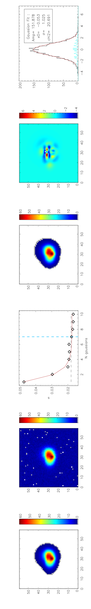
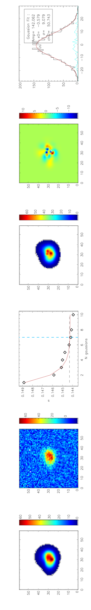
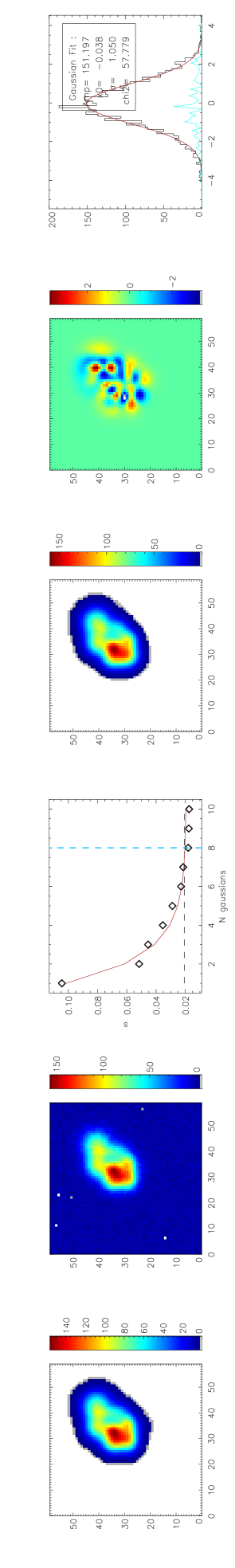
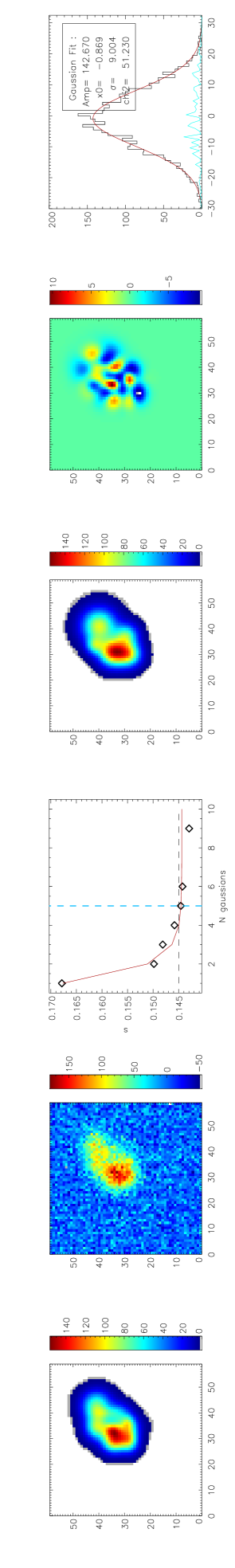
Figure 1: Main results for the two sets of simulations described in Section IV (first two rows simulations 1a and 1b, last two rows simulations 2a and 2b). From left to right for each row : the initial simulated beam pattern, id + noise, the quadratic deviation $S$ as a function of the number of Gaussians, the best-fit model for the beam pattern, the residual map after substraction of the input noise in percents and the histogram of the residual map including input noise. The dot blue lines show the computed number of Gaussian necessary to reproduce the initial simulated beam. The histogram of the residual map is fitted with a Gaussian (in red), the difference is shown in blue.

We consider now the two sets of simulations (simulations 1a, 1b, 2a and 2b) described in Section III. The fit is performed using a least square fit in the non-linear case following the algorithm described in brandt . Figure 1 presents the main results for these two sets of simulations : the first two rows for simulations 1a and 1b, and the last two rows for simulations 2a and 2b. In each case, we have plotted, from left to right :

• the initial simulated beam pattern

• the initial simulated beam pattern + noise

• the quadratic deviation $S$ as a function of the number of Gaussians $N$ (the dotted line represents the number of Gaussians chosen for the final beam pattern model)

• the best-fit model for the beam pattern

• the residual map after substraction of the input noise in percents

• the histogram of the residual map including input noise, fitted to a Gaussian (in red) with residuals to the Gaussian (in blue)

The distribution of $S(N)$ is modelled by a decreasing exponential, $exp(-\tau N)$, plus a constant $k$. The number of Gaussians $N$ is chosen such that $N$ is the smaller value verifying

$$S(N)-k<\frac{t}{\tau}$$ (4)

where $t$ is a threshold defined by the user for the required precision.

Figure 1 shows that a small number of Gaussians is enough for a good fit (typically less than 10 Gaussians give less than 2 % residuals). In some cases, the algorithm does not converge and therefore no data point is plotted on the figure. Lack of convergence may appear for some combination of number of Gaussians. This is generally solved by using a smaller or larger number of Gaussians in the fit.

The efficiency of the fit is illustrated by the distribution of the residuals which are very close to the white noise distribution centered at zero with the dispersion corresponding to the level of the input noise. Note also that the reconstructed beams are marginally sensitive to the noise level and that the apparent decomposition in three different peaks (case 1b) leads to residuals with amplitude only of the level of the noise.

Once the Gausssians parameters have been estimated, map simulations using any pointing strategy can be done quickly and precisely.

V Accuracy of the Asymfast method

In this section, we compare the accuracy of Asymfast to that of other common approaches including the modelling of the beam pattern either by a single circular Gaussian or by an elliptical Gaussian. We use as a reference the brute-force convolution with the true beam pattern at each pointing direction.

For this purpose, we have convolved, using the different methods described before, a map containing 26 point sources with the same amplitudes uniformly distributed over half an hemisphere. The level of accuracy for each of the former methods of convolution is estimated by computing the quadratic deviation of the convolved map obtained for that particular method with respect to the convolved map obtained by brute-force convolution.

beam	1 circular	1 elliptical	asymfast
simulation	Gaussian	Gaussian	(N Gaussians)
1a	4.444	1.187	0.734 (7)
1b	4.420	1.281	0.936 (7)
2a	10.513	4.095	0.826 (8)
2b	10.464	4.154	1.455 (5)

Table 1: Accuracy of the three methods discussed in the text (see Section V) for each set of simulations.

Table 1 represents the quadratic deviation for each of the methods as a percentage of the maximum of the original point-sources map. This quantity can be interpreted as the percentage of spurious noise introduced by the convolution method. In the case of quasi-circular beams (simulations 1a and 1b), Asymfast is 1.5 (resp. 6) more accurate than the elliptical (resp. circular) approximation. For more realistic irregular beams (simulations 2a and 2b), Asymfast is about 4 (resp. 10) times more accurate than the elliptical (resp. circular) approach. Moreover Asymfast depends neither on the shape of the beam pattern nor on the noise level.

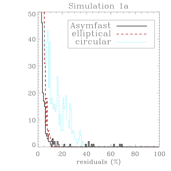
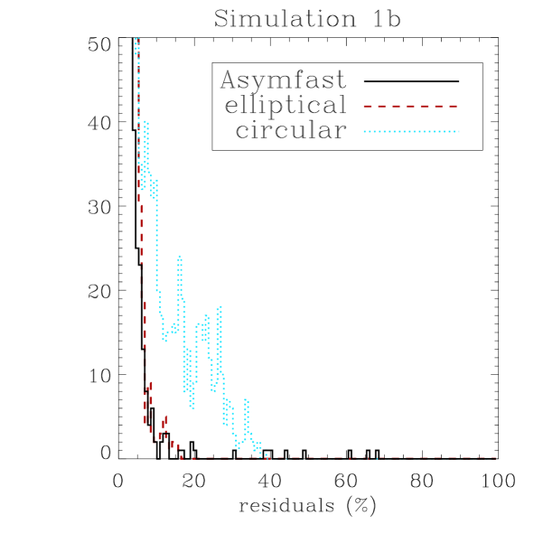
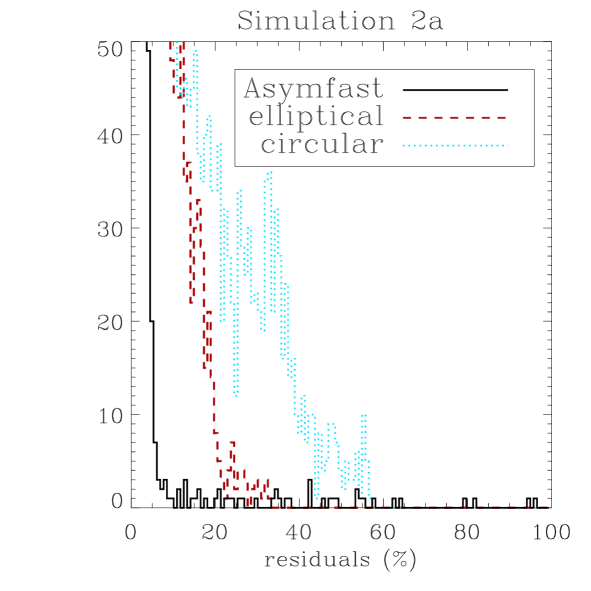
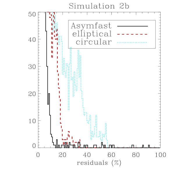
Figure 2: Histogram of the percentage of the quadratic deviation residual maps for the Asymfast (solid line), elliptical (dashed line) and circular (dotted line) approximations. Top panel : simulations 1a, 1b. Bottom panel : simulations 2a, 2b.

Figure 2 shows, for the two sets of simulations considered (simulations 1a, 1b on the top panel and simulations 2a, 2b and the bottom panel), the histogram of the percentage of the quadratic deviation residual maps for the Asymfast (solid line), elliptical (dashed line) and circular (dotted line) approximations. The figure confirms the results shown in Table 1, indicating that Asymfast is a very good approximation to both quasi-circular and irregular beams (residuals smaller than 5%). By contrast, the elliptical approximation can only be safely used in the case of quasi-circular beams (residuals about 20% for simulations 2). The circular approximation, as expected, is very poor in any case (residuals of the order 40%).

In conclusion, the Asymfast results are very close to the standard solution while the circular and elliptical Gaussian approximations are very poor for realistic beam patterns. In addition, the standard approach, which works in real-space, necessarily uses a beam pattern with fixed resolution. By contrast, Asymfast works in the spherical harmonic space where the resolution is only limited by the pixelisation of the sky map. Moreover, Asymfast can obtain full resolution in frequency with no mixing. Obtaining the same frequency resolution with brute-force convolution requires a full-sky beam pattern which increases considerably the computing time.

VI Time-computing efficiency of Asymfast vs brute-force convolution

As discussed in the following section, the determination in the spherical harmonic space of the effective circular transfer function of an asymmetric beam pattern, $B_{\ell}^{eff}$, requires a large number (of the order of 1000) of accurate Monte-Carlo simulations of fake data appropriately convolved by the instrument beam. Therefore, any algorithm used for this purpose need to be much faster than the brute-force convolution procedure to keep the computing time reasonable.

To quantify the time-computing efficiency of Asymfast, we consider $n_{simu}=1000$ Monte-Carlo simulations of a convolved full-sky map for a single Planck-like detector. We use a squared map of $n_{beam}=3600$ pixels to describe the beam pattern and simulated timelines for 12 months of Planck observations which correspond to $n_{scan}=5\ 10^{9}$ samples. With Asymfast, we model the beam pattern using $N=10$ Gaussians. For each simulation, the total number of pixels on the full-sky map is $n_{pix}=12*N_{side}^{2}$ for three values of $N_{side}$ : 256, 512 and 1024 considered.

Nside	HEALPix	Asymfast	brute-force
	1 Gaussian	10 Gaussians	convolution
256	0.127	7.40	171
512	1.02	29.1	1340
1024	8.13	203	10700

Table 2: Computing-time, in terms of $10^{6}$ arbitrary CPU-units and including the input/output time access, for circular beam convolution in the harmonic space using the HEALPix package, and for asymmetric beam convolution using Asymfast and brute-force convolution algorithms. We have considered a set of 1000 simulations as described in Section VI.

For these simulations, Table 2 shows the computing-time, in terms of arbitrary CPU-units, for circular beam convolution in the harmonic space using the HEALPix package, and for asymmetric beam convolution using Asymfast or brute-force convolution algorithms.

We observe that Asymfast is more than 50 times faster than the brute-force convolution for the high resolutions ($N_{side}=512$ ou $1024$). This is because the convolution in the spherical harmonic space used by Asymfast is much faster than in real space. In addition, Asymfast is particularly efficient for Monte-Carlo purposes because the beam modelization and the computing of the pointing directions corresponding to each of the $N$ sub-beam are performed only once.

Furthermore, for high resolutions, the Asymfast computing-time is just a factor of 2 larger than the computing-time needed for the convolution of $N$ circular Gaussians in spherical harmonic space. The extra computing time with respect to the convolution of $N$ circular Gaussians comes from the projection and the deprojection operations performed by Asymfast.

Finally, the difference in computing-time between Asymfast and the brute-force convolution also increases with the beam map resolution as the second method depends linearly on beam map number of pixels while Asymfast is very marginally sensitive to it, only at the beam fit step.

VII Application to CMB analysis : estimation of the beam transfer function $B_{\ell}$

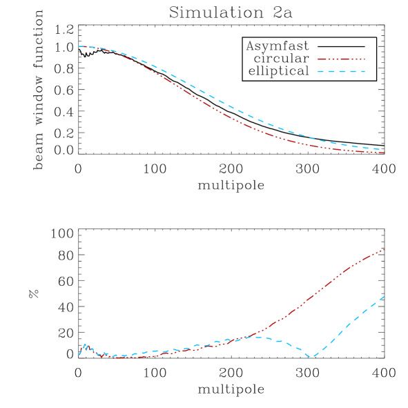
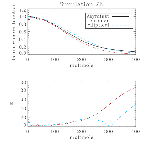
Figure 3: Beam transfer functions and variations with respect to Asymfast for the two sets of simulations (simulations 1a, 1b, 2a and 2b). The Monte-Carlo estimation using Asymfast described in Section VII (solid line) is compared to the analytic transfer function of a circular approximation of the beam (semi-dashed line) and to the elliptical approximation to order 4 from pablo (dashed line). The top panel represents the beam transfer functions whereas the bottom panel shows the differences to the Asymfast estimation for the other two approximations.

In this section, we describe how Asymfast can be used to estimate this effective circular transfer function for realistic asymmetric beams. A beam is described in the spherical harmonic space by a set of coefficients $b_{\ell m}$ for each scanning orientation at each pointing position. The Gaussianity of the primordial fluctuations of the CMB is a key assumption of modern cosmology, motivated by simple models of inflation. So the angular power spectrum of the CMB should be a circular quantity and it is common to just consider an effective circular beam transfer function, $B_{\ell}^{eff}$. The “circularization”of the beam may be obtained by several ways : assuming a Gaussian beam (the easiest way, leading to a simple analytic description), computing the optimal circularly symmetric equivalent beam (wu , applied to Maxima) or fitting the radial beam profile by a sum of Hermite polynomials (page , applied to WMAP). The analytic expression of the beam transfer function of elliptical Gaussian beams has also been studied in details by pablo and by souradeep who applied it to Python V.

With Asymfast, the “circularization”of the beam depends on the scanning strategy as it is computed on the map after convolution by the asymmetric main beam. So it is comparable to or more precise than other methods, depending on how the scans intersect each other.

For a circular Gaussian beam (angles $\theta$ and $\phi$ corresponding to the beam direction),

$$b(\theta,\phi)=\frac{1}{2\pi\sigma^{2}}\exp\left[-\frac{\theta^{2}}{2\sigma^{2}}\right],$$ (5)

the beam transfer function in case of a pixel scale much smaller than the beam scale is approximated by white

$$B_{\ell} = \exp\left[-\frac{1}{2}\ell(\ell+1)\sigma^{2}\right].$$ (6)

Note that in this case, the beam transfer function does not depend on the orientation of the beam on the sky and is given by a simple analytical expression.

For a moderate elliptical Gaussian beam pattern, we can compute an analytic approach pablo to the beam transfer function by introducing a small perturbation to Eq. 5 so that

$$b^{ell}(\theta,\phi)=\frac{1}{2\pi\sigma^{2}}\exp\left[-\frac{\theta^{2}}{2\sigma^{2}}f(\phi)\right]$$ (7)

where $f(\phi)$ describes the deviation from circularity.

For general irregular asymmetric beams, the previous approximation is not well adapted and the orientation of the beam on the sky has to be taken into account. For this purpose, we estimate an effective beam transfer function, $B_{\ell}^{eff}$, from Monte-Carlo simulations which use the Asymfast method for convolution as follows :

1. We convolve CMB simulated maps by the beam pattern using Asymfast.

2. For each simulation, we estimate a $B_{\ell}^{eff}$ inverting the equation master

   $$\tilde{C}_{\ell}=M_{\ell\ell^{\prime}}{B_{\ell^{\prime}}^{eff}}^{2}C_{\ell^{\prime}}$$

   where $M_{\ell\ell^{\prime}}$ is the coupling kernel matrix that takes into account the non-uniform coverage of the sky map, $\tilde{C}_{\ell}$ is the pseudo-power spectrum computed on the convolved map and $C_{\ell}$ is the input theorical model.

3. We compute the effective transfer function of the beam, by averaging the $B_{\ell}^{eff}$ obtained for each of the simulations.

We have tested this method on simulations of pure circular Gaussian beams for which we have obtained a beam transfer function fully compatible with Eq. 6 as expected.

Figure 3 shows the estimate of the effective beam transfer function $B_{\ell}^{eff}$ for the two sets of beam simulations discussed in the previous sections (simulations 1a, 1b, 2a, 2b) using a Monte-Carlo of 25 simulations. The results of this Monte-Carlo (solid line) is compared to the analytic transfer function of a circular approximation of the beam (semi-dashed line) and to the elliptical approximation computed from pablo (dashed line). The top panel represents the beam transfer functions whereas the bottom panel shows the differences to the Asymfast estimation for both analytical approximations (circular, semi-dashed line and elliptical, dashed line). The Asymfast effective beam transfer function shows some irregularities at very low $\ell$ due to the cosmic variance.

As expected, for the quasi-circular beam (simulations 1a and 1b), the estimate transfer functions for the three methods are similar within 10 %. The differences observed between our approach and the elliptical approximation are mainly due to the fact that the latter does not take into account the scanning strategy. Due to the complex but realistic scanning strategy used in our simulations, we expect that, in general, a given position on the sky will be observed with different relative beam orientations and therefore the effective beam will appear more circular.

By contrast, for a more irregular beam pattern (simulations 2a and 2b), the differences between the three methods are much larger (from 10 % at low $\ell$ up to 70 % at high $\ell$). The beam transfer function obtained using the elliptical approximation follows better the one obtained using Asymfast. We expect that the complex scanning strategy would make the effective beam more circular. However as the beam pattern is very asymmetric, the effective beam will contain complex highly irregular structures which cannot be mimicked by an oriented elliptical beam. Therefore, the largest differences are found at high resolution.

Note that the results presented here are also valid for higher resolution beams. For this paper, we have considered low resolution beams to be able to directly compare the Asymfast convolution to standard brute-force convolution.

VIII Application to Archeops

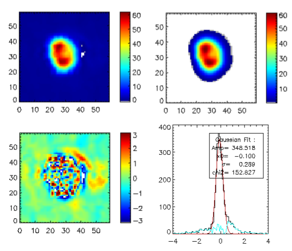
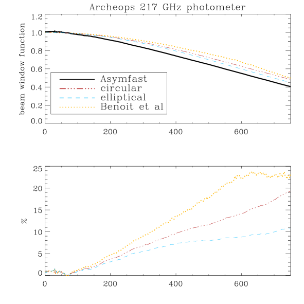
Figure 4: From left to right and from top to bottom. Main beam map of the 217 GHz photometer used in the first Archeops CMB analysis and its reconstruction with Asymfast using 10 Gaussians the $B_{\ell}^{eff}$; the residuals-map to this one and the residuals histogram; the beam transfer function for the Gaussian approximation, for the simulations as done in [6] and for Asymfast; relative differences to the Asymfast beam transfer function estimatate for the other three approaches. See text for details.

Asymfast has been applied to the main beam of the Archeops bolometers which are identical to the Planck-HFI ones. The beam shapes were measured on Jupiter beamarcheops and are for most of them moderately elliptical, the multimode ones being rather irregular. Figure 4 shows the study of the Archeops 217 GHz photometer used for the first Archeops CMB analysis archeops . On the first row we show the $1\times 1$ deg with 1 arcminute pixel maps of the main beam, at left the initial map, at right the reconstructed one with 10 Gaussians. The second row presents the residual map and its histogram. The latter is fitted with a Gaussian (in red), the difference to it is shown in blue. The Monte-Carlo estimation using Asymfast described in Section VII (solid line) is compared to the analytic transfer function of a circular approximation of the beam (semi-dashed line), to the elliptical approximation to order 4 from pablo (dashed line) and to the estimation obtained by simulation used in archeops (dotted line). They are shown on the third row figure. The bottom panel shows the differences to the Asymfast beam transfer function estimation for the other three approaches.

The beam is well reproduced as the residual map do not exhibit any structure. Moreover the dispersion of the distribution of the residuals is compatible to the noise level of the initial map. The deviation to the Gaussian and to the elliptical models arises from $\ell\approx 200$, i.e. the top of the first acoustic peak and culminates around $\ell\approx 500-600$, i.e. at the second peak location. Therefore the fine structure of main beams with equivalent FWHM of 13 arcminutes is already determinant for the measurement of the second acoustic peak with Archeops. Because of the irregularity of the beam, we are more sensitive to higher resolution structures.

IX Conclusions

Asymfast is a fast and accurate convolution procedure particularly well-adapted to asymmetric beam patterns and complex scanning strategies which are often used in CMB observations. Asymfast can both produce convolved maps from input timelines and compute, from Monte-Carlo simulations, an accurate circular approximation to the transfer function, $B_{\ell}^{eff}$, of any asymmetric beam pattern. The computing time needed to obtain a convolved map is dominated by the HEALPix software computing time. So it scales as ${{\cal O}\!\left(n_{pix}^{3/2}\right)}$ where $n_{pix}$ is the number of pixels of the map, with a multiplying factor depending on the number of Gaussians.

Asymfast models any general beam pattern by a linear combination of circular 2D Gaussians, permitting an accurate reconstruction of the instrumental beam, with residuals smaller than 1 % (compared to 4 % for an elliptical Gaussian model). In addition, Asymfast convolution is at least a factor of 50 faster than the brute-force convolution algorithm for full-sky maps of 12.5 million pixels and even faster at higher resolution. This allows us to perform a large number of Monte-Carlo simulations in a reasonable computing time to estimate accurately the effective circular transfer function of the beam pattern.

By constrast to other modelling techniques like page and pablo , Asymfast can be used with non-circular and non-elliptical beam patterns. Furthermore Asymfast approximates the main beam pattern while wandelt uses an exact 4-$\pi$ beam description, nevertheless it can be equally easily applied to any general scanning strategy while the feasibility of wandelt strongly depends on the former challinor .

Note that Asymfast is a general convolution algorithm which can be also used successfully in many other astrophysical areas to reproduce the effects of asymmetric beam patterns on sky-maps and to compare observations from independant instruments which requires the cross-convolution of the datasets. Any circular functions with analytic description in the harmonic space may be used instead of 2D symmetric Gaussians.