The magnetic field of M 31 from multi-wavelength radio polarization observations

The configuration of the regular magnetic field in M 31 is deduced from radio polarization observations at the wavelengths $\lambda\lambda\ 6,\ 11$ and $20\,{\rm cm}$. By fitting the observed azimuthal distribution of polarization angles, we find that the regular magnetic field, averaged over scales 1–3 kpc, is almost perfectly axisymmetric in the radial range $8$ to $14\,{\rm kpc}$, and follows a spiral pattern with pitch angles of $p\simeq-19\degr$ to $p\simeq-8\degr$. In the ring between $6$ and $8\,{\rm kpc}$ a perturbation of the dominant axisymmetric mode may be present, having the azimuthal wave number $m=2$. A systematic analysis of the observed depolarization allows us to identify the main mechanism for wavelength dependent depolarization – Faraday rotation measure gradients arising in a magneto-ionic screen above the synchrotron disk. Modelling of the depolarization leads to constraints on the relative scale heights of the thermal and synchrotron emitting layers in M 31; the thermal layer is found to be up to three times thicker than the synchrotron disk. The regular magnetic field must be coherent over a vertical scale at least similar to the scale height of the thermal layer, estimated to be $h_{\mathrm{th}}\simeq 1\,{\rm kpc}$. Faraday effects offer a powerful method to detect thick magneto-ionic disks or halosaround spiral galaxies.

1 Introduction

The Andromeda nebula, M 31, is the nearest spiral galaxy to the Milky Way. Despite its high inclination to the line of sight, the large angular size of the galaxy allows detailed studies of its magnetic field and interstellar medium (ISM). In particular, the large scale morphology of the magnetic field can be investigated with unmatched precision. M 31 is thus of prime importance in bringing together observational data and theory about galactic magnetic fields.

Early radio wavelength observations of M 31 at $\lambda 73\,{\rm cm}$ (Pooley Pooley69 (1969)) and $\lambda 11\,{\rm cm}$ (Berkhuijsen & Wielebinski Berkhuijsen74 (1974), Berkhuijsen Berkhuijsen77 (1977)) show the continuum emission concentrated in a ring, at a radius of $r\simeq 50\arcmin\simeq 10\,{\rm kpc}$. The first radio polarization observations at $\lambda 11\,{\rm cm}$, using the 100m Effelsberg telescope (Beck et al. Beck78 (1978)), indicated that the magnetic field in the southern part of M 31 is aligned with the optical spiral arms. Beck (Beck82 (1982)) interpreted the $\lambda 11\,{\rm cm}$ data by comparing the observed polarization angles with a model of the polarized emission to reveal a predominantly azimuthal large-scale magnetic field, concentrated in the $r\simeq 10\,{\rm kpc}$ ‘ring’, directed in the same direction as the rotation of the galaxy. Faraday rotation measures (RMs) from polarization observations of the southwestern arm of M 31 at $\lambda\lambda 6,20\,{\rm cm}$ confirmed the presence of a basically axisymmetric spiral magnetic field (Beck et al. Beck89 (1989)). A bisymmetric component of the magnetic field was suggested by Sofue & Beck (Sofue87 (1987)) from an analysis of the deviation of the polarization angles at $\lambda 11\,{\rm cm}$ from those expected due to a purely axisymmetric regular magnetic field; however it is not clear whether the inferred bisymmetric mode is statistically significant. Ruzmaikin et al. (Ruzmaikin90 (1990)) modelled the $\lambda 11\,{\rm cm}$ polarization angles of M 31 with an azimuthal Fourier expansion for the regular magnetic field and ascertained that deviations of the magnetic field from axial symmetry are evident statistically and may indicate bisymmetric or higher modes. More recently, RMs of 21 background radio sources in the field of M 31 were found to be compatible with the same magnetic field structure, but extending far away from the $r\simeq 10\,{\rm kpc}$ ‘ring’, probably to $5\lesssim r\lesssim 25\,{\rm kpc}$ (Han et al. Han98 (1998)). This remains to be substantiated with a statistically significant number of sources.

Recently, Berkhuijsen et al. (Berkhuijsen03 (2003)) presented a new $\lambda 6\,{\rm cm}$ survey of M 31 and concluded that: the regular component of the magnetic field is probably as strong as the turbulent field; the regular magnetic field has an average pitch angle of $\simeq-15\degr$ in the range $8\lesssim r\lesssim 12\,{\rm kpc}$, with a negative value indicating a trailing spiral; gradients in Faraday rotation measure may be an important cause of depolarization.

In this paper we seek to take the next logical step in understanding the magnetic structure of M 31 by developing a detailed and self-consistent description of the magnetic field. We use all of the radio polarization surveys ($\lambda\lambda 6,11,20\,{\rm cm}$) and fit together information on polarization angles, Faraday rotation, non-thermal radio emission intensities, depolarization and the scale heights of ISM components. Our analysis has two main components: deducing the large-scale geometry of the magnetic field and deriving parameters of the magneto-ionic ISM from analysis of depolarization of the synchrotron emission. Our approach is the latest in a sequence of methods used to interpret radio polarization observations of external galaxies. Ruzmaikin et al. (Ruzmaikin90 (1990)) considered the variation of polarization angles at a single wavelength, Sokoloff et al. (Sokoloff92 (1992)) extended this approach to multiple wavelengths and Berkhuijsen et al. (Berkhuijsen97 (1997)) introduced variation in the intrinsic angle of polarized emission in a galaxy. We develop a new model, by combining an analysis of multi-wavelength polarization angles – based on the earlier methods – with modelling of the wavelength dependent depolarization.

A short description of the data we use is presented in Sect. 2. The properties of the synchrotron disk are discussed in Sect. 3. In Sect. 5 we use polarization angles at $\lambda\lambda 6,11,20\,{\rm cm}$ to deduce the three-dimensional structure of the regular magnetic field in M 31. The method, developed from that used by Berkhuijsen et al. (Berkhuijsen97 (1997)) to determine the regular magnetic field of M 51, takes into account the intrinsic angle of polarized emission in the disk of M 31, Faraday rotation by the magneto-ionic medium in M 31 and Faraday rotation in the Milky Way. In Sect. 6 we analyze the radial and azimuthal variation in the depolarization between wavelengths $\lambda 6\,{\rm cm}$ and $\lambda 20\,{\rm cm}$, and derive constraints on the scale heights of the thermal and synchrotron emitting disks of M 31. This demonstrates a new and potentially powerful method for extracting such information from radio polarization observations of spiral galaxies. A short discussion of the preliminary results was presented in Fletcher et al. (Fletcher00 (2000)).

2 Observational data

2.1 Radio continuum emission at $\lambda\lambda$6, 11 and 20 cm

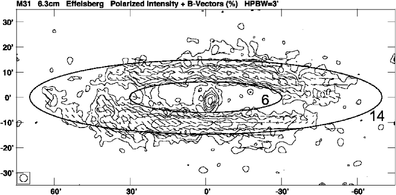
Figure 1: Polarized intensity (contours) of M 31 with the orientation of the emission B-vector also shown (dashes, not corrected for Faraday rotation) with their lengths proportional to the degree of polarization, observed at $\lambda 6\,{\rm cm}$ with the Effelsberg radio telescope (Berkhuijsen et al. Berkhuijsen03 (2003)). Note that the foreground RM of $-90\,{\rm rad\,m^{-2}}$ (Table 2) corresponds to Faraday rotation of about $20\degr$ so that the intrinsic B-vectors are roughly azimuthal. The beam width is $3\arcmin$ and the rms noise is 0.2 mJy/beam. Contour levels are $1,2,3,4,6\times(5\times 10^{-4})$ Jy/beam. A length of B-vectors of $3\arcmin$ corresponds to a degree of polarization of 36%. The northern major axis is to the left and the ellipses show the radial range of the data analyzed in this paper, $6\leq r\leq 14\,{\rm kpc}$.

For the analysis in this paper we adopt the following parameters of M 31: a distance of $690\,{\rm kpc}$ ($1\arcmin=196\,{\rm pc}$ on the major axis), a centre position of $\rm RA_{50}=0^{h}40^{m}1\aas@@fstack{s}8,\ DEC_{50}=40\degr 59\arcmin 46\arcsec$, an inclination angle of $i=78\degr$ (Braun Braun91 (1991)) where $0\degr$ is face-on, and a position angle of the northern major axis of $37\degr$.

Berkhuijsen et al. (Berkhuijsen03 (2003)) observed a field of $150\arcmin\times 70\arcmin$ at $\lambda 6.2\,{\rm cm}$ with the 100m Effelsberg telescope . The original resolution was $2\aas@@fstack{\prime}4$. Figure 1 shows the polarized intensity smoothed to a beamwidth of $3\arcmin$, along with ellipses showing the radial range considered in this paper. Preliminary results were also discussed by Han et al. (Han98 (1998)) and Beck (Beck00 (2000)).

The $\lambda 11.1\,{\rm cm}$ map of M 31 was obtained with the Effelsberg telescope and was published by Beck (Beck82 (1982)). The original resolution of $4\aas@@fstack{\prime}4$ was smoothed to $5\arcmin$ for this paper. The VLA map at $\lambda 20.5\,{\rm cm}$ by Beck et al. (Beck98 (1998)) has an original resolution of $45\arcsec$, used in the analysis of polarization angles in Sect. 5. For the comparison of polarized intensities at $\lambda\lambda 6,20\,{\rm cm}$ presented in Sect. 6, the $\lambda 20\,{\rm cm}$ map was smoothed to $3\arcmin$, the same as the $\lambda 6\,{\rm cm}$ map. Since we are interested in wavelength dependent effects (Faraday depolarization) we require the same degree of wavelength independent depolarization at $\lambda 6\,{\rm cm}$ and $\lambda 20\,{\rm cm}$ and so the resolutions must be the same (wavelength independent depolarization arises from unresolved fluctuations of the polarized emission – see Appendix A).

From the $\lambda 20\,{\rm cm}$ map in total intensity, smoothed to a resolution of $3\arcmin$, and the $\lambda 6\,{\rm cm}$ total intensity map at the same resolution Berkhuijsen et al. (Berkhuijsen03 (2003)) computed a spectral index map and maps of thermal and non-thermal emission at these wavelengths. Combination of the polarized and non-thermal emission at each wavelength then yields the non-thermal degrees of polarization that are analyzed in Sect. 6.

Missing spacings affect the diffuse emission at $\lambda 20\,{\rm cm}$ detectable by the VLA. This was corrected in total intensity with the help of Effelsberg data at the same wavelength. A further complication is that M 31 lies behind a spur of the Milky Way seen in $\lambda 20\,{\rm cm}$ non-thermal emission (see., e.g., Gräve et al. Graeve81 (1981), Beck et al. Beck98 (1998)). The total emission from the foreground at $\lambda 20\,{\rm cm}$ was removed using an Effelsberg map of the extended region of sky in the direction of M 31, but the polarized emission cannot be separated into Milky Way and M 31 components so that a correction for missing spacings was not possible in the maps of Stokes $Q$ and $U$ (Beck et al. Beck98 (1998)). However, strong spatial variation in the Faraday rotation intrinsic to M 31, shown in Figure 7 for RM derived using $\lambda\lambda 6,11,20\,{\rm cm}$ data means that at $\lambda 20\,{\rm cm}$ Stokes $Q$ and $U$ originating from M 31 will change rapidly with position and hence the effect of missing spacings is probably small for the emission from M 31. Note that a similar pattern is present when RM is determined using only $\lambda\lambda 6,11\,{\rm cm}$ (Fig. 12 in Berkhuijsen et al. Berkhuijsen03 (2003)).

2.2 Data averaging in rings and sectors

The maps in the Stokes parameters $I$, $Q$ and $U$, at each of the three wavelengths, were averaged in sectors of $20\degr$ azimuthal and $2\,{\rm kpc}$ radial width, in the range $6\leq r\leq 14$. The size of the sectors was chosen to match the resolution of the data at $\lambda 6\,{\rm cm}$. Next we describe how the average $Q$ and $U$ intensities in each sector were combined to give the average polarization angle and the average polarized emission intensity in each sector.

2.2.1 Polarization angles

The polarization angle in a individual sector was calculated as $\psi=\frac{1}{2}\arctan{\langle U\rangle}/{\langle Q\rangle}$, where $\langle\dots\rangle$ denotes the average value of the parameter over the pixels within a sector. The resolutions used were $3\arcmin$, $5\arcmin$ and $45\arcsec$ at the wavelengths $\lambda\lambda 6,11,20\,{\rm cm}$ respectively. The errors in polarization angle were computed as the standard deviations, within one sector, between all pixels whose intensity is stronger than three times the rms noise level. If the number of pixels in a sector was below five, the error was calculated by averaging several adjacent sectors (this procedure was suggested by Berkhuijsen et al. Berkhuijsen97 (1997)). For two measurements (both at $\lambda 20\,{\rm cm}$, in the ring 6–8 kpc at $\theta=120\degr$ and in the ring 8–10 kpc at $\theta=60\degr$) the error thus obtained was less than the noise in the maps and here the noise error was taken. These average polarization angles are analysed in Sect. 5.

The $\lambda 20\,{\rm cm}$ polarized emission from M 31 is mixed with a substantial amount of emission from the Milky Way foreground. At $45\arcsec$ resolution the polarized emission from the M 31 ‘ring’ and nucleus is clearly visible and the polarization angles are clustered in coherent cells, sometimes connected with the position of OB associations in M 31 (see Figs. 2 and 6 of Beck et al. Beck98 (1998)). Thus, the average $\lambda 20\,{\rm cm}$ polarization angles in sectors with a surface area several tens of times larger than the $45\arcsec$ resolution, are a reliable measure of the emission from M 31 at this wavelength. The foreground Milky Way emission merely contributes to the dispersion of angles in a given sector and hence to the standard deviation used as our error estimate.

A further check is applied, by repeating the modelling described in Sect. 5 using only the $\lambda\lambda 6,11\,{\rm cm}$ data. The character of the deduced regular magnetic field does not substantially change if the $\lambda 20\,{\rm cm}$ is excluded, though naturally the parameters are less well defined.

2.2.2 Polarized intensities

We define the average polarized emission of a sector as $PI=\left(\langle Q\rangle^{2}+\langle U\rangle^{2}-1.2\sigma_{Q,U}^{2}\right)^{1/2}$, where $\sigma_{Q,U}$ is the rms noise in $Q$ and $U$ and provides an approximate correction for positive bias in $PI$ (Wardle & Kronberg Wardle74 (1974)). The $Q$ and $U$ intensities of all pixels in a sector were averaged to compute $PI$. Errors in non-thermal and polarized intensities were estimated as the standard deviation between all pixels in a sector as described in Sect. 2.2.1.

In Sect. 6 we compare the degree of polarization at $\lambda 20\,{\rm cm}$, where Faraday effects are strong, with that at $\lambda 6\,{\rm cm}$, where minimal Faraday rotation occurs. It is necessary to smooth the $\lambda 20\,{\rm cm}$ map to the $3\arcmin$ resolution of the $\lambda 6\,{\rm cm}$ for this analysis. When smoothed to a resolution of $3\arcmin$ the ’ring’ like polarized emission from M 31 becomes less distinct than at $45\arcsec$ and narrow strips of zero polarized intensity become apparent in the $\lambda 20\,{\rm cm}$ map. These ‘canals’ are interpreted as depolarization effects in the foreground polarized emission of the Milky Way by Shukurov & Berkhuijsen (Shukurov03 (2003)). The ‘contamination’ of the $3\arcmin$ resolution polarized intensity by Milky Way emission is therefore probably more serious than for the polarization angles. The azimuthal pattern of the degree of polarization at $\lambda 11\,{\rm cm}$ is somewhat similar to that at $\lambda 20\,{\rm cm}$. However, the difference in the degrees of polarization at $\lambda 11\,{\rm cm}$ and $\lambda 6\,{\rm cm}$ is not large enough to allow detailed modelling as a check on our results in Sect. 6. Therefore, the observed $\lambda 20\,{\rm cm}$ polarized intensities are an upper limit on the emission from M 31.

3 The non-thermal disk

Table 1: Properties of the synchrotron disk in M 31

$r$	$I_{6}$	$P_{6}$	$\,B_{\mathrm{tot}}$	$\,B$	$\,b$	$h_{6}$	$h_{20}$
(kpc)	(mJy/beam)	(%)	($\mu$G)	($\mu$G)	($\mu$G)	(pc)	(pc)
6–18	3.72$\pm$0.06	30$\pm$1	7.3	4.9	5.4	220	290
8–10	4.71$\pm$0.05	33$\pm$1	7.5	5.2	5.4	240	330
10–12	4.19$\pm$0.05	31$\pm$1	7.1	4.9	5.2	270	360
12–14	2.71$\pm$0.05	35$\pm$1	6.3	4.6	4.3	290	390

Notes: $r$ is the radial range, $I_{6}$ the average non-thermal radio intensity per beam area at $\lambda 6\,{\rm cm}$ (HPBW=$3\arcmin$), $P_{6}$ the non-thermal degree of polarization at $\lambda 6\,{\rm cm}$ obtained from the average polarized intensity per beam area divided by $I_{6}$; $h_{6}$ and $h_{20}$ the exponential scale heights of the synchrotron emission at $\lambda 6\,{\rm cm}$ and $\lambda 20\,{\rm cm}$, respectively; $\,B_{\mathrm{tot}}$, $\,B$ and $\,b$ are the average equipartition strengths of the total, regular and turbulent fields, respectively. The uncertainty in the derived field strengths is about 20%. See Sect. 3 for further explanations.

Our analysis of depolarization in Sect. 6 requires an estimate of the scale height of the non-thermal disk and the discussion of the regular magnetic field, revealed by our model in Sect. 5, is aided by an estimate of the magnetic field strengths based on equipartition arguments. In this section we derive both of these quantities.

3.1 The scale height of the non-thermal emission

In a study of an arm region in the southwest quadrant of M 31 Berkhuijsen et al. (Berkhuijsen93 (1993)) found that the half-width of the arms at $\lambda 20\,{\rm cm}$ in the plane of the sky is equal to that of the total neutral gas (H i+2H₂) suggesting similar scale heights for radio continuum emission at $\lambda 20\,{\rm cm}$ and neutral gas.

We cannot yet check this for other regions in M 31, but we can compare the scale heights at $\lambda 20\,{\rm cm}$ derived by Moss et al. (Moss98 (1998)) with the scale heights of H i given by Braun (Braun91 (1991)). Moss et al. (Moss98 (1998)) determined the scale height of the continuum emission from four cuts parallel to the minor axis going through the bright ‘ring’ at about $20\arcmin$ on either side of the centre. The arms were cut at radial distances between 6 and $11\,{\rm kpc}$, and the mean of the exponential scale heights is $325\pm 43\,{\rm pc}$. Braun (Braun91 (1991)) described the exponential scale height of the H i emission as $h_{\mathrm{HI}}=(182\pm 37)+(16\pm 3)\,r$, where the radius $r$ is in kpc and $h_{\mathrm{HI}}$ in pc. For the same positions as the radio continuum cuts, the mean scale height of H i is $310\pm 45\,{\rm pc}$. Hence, the scale height of the radio continuum emission at $\lambda 20\,{\rm cm}$ is the same as that of H i within errors. At this wavelength the width of the radio continuum emission is determined by the synchrotron emission, because the thermal emission is weak and has a narrower distribution (Berkhuijsen et al. Berkhuijsen00 (2000)). Therefore we take the synchrotron scale height at $\lambda 20\,{\rm cm}$ equal to the H i scale height as given by Braun (Braun91 (1991)).

The synchrotron scale height depends on frequency as $\nu^{-0.25}$, as observed in NGC 891 (Hummel et al. Hummel91 (1991)) and M 31 (Berkhuijsen et al. Berkhuijsen91 (1991)), thus the scale heights at $\lambda 11\,{\rm cm}$ and $\lambda 6\,{\rm cm}$ are somewhat smaller than at $\lambda 20\,{\rm cm}$ (see Table 1).

3.2 The equipartition magnetic field strength

The transverse component of the total field strength $\,B_{\mathrm{tot\perp}}$ (the quadratic sum of the regular and turbulent components) can be evaluated from the intensity of the non-thermal emission assuming, for example, equipartition between the energy densities of magnetic field and cosmic rays (see Pacholczyk Pacholczyk70 (1970), Longair Longair94 (1994)). However, we use a fixed integration interval in cosmic-ray energy rather than a fixed interval in radio frequency (see Beck et al. Beck96 (1996)). In this case, and for a non-thermal spectral index $\alpha_{\mathrm{n}}\simeq 1$, the equipartition field strength is identical to the minimum-energy field strength. The polarized intensity yields the strength of the transverse regular field, $\,B_{\perp}$; the transverse turbulent field strength $\,b_{\perp}$ is then found from $\,b_{\perp}^{2}=\,B_{\mathrm{tot\perp}}^{2}-\,B_{\perp}^{2}$. The values of $\,B_{\mathrm{tot}}$ and the regular field strength $\,B$ one obtains by deprojection assuming that $\,B$ is oriented parallel to the plane of M 31, and $\,b=\left(\frac{3}{2}\,b_{\perp}^{2}\right)^{1/2}$ assuming statistical isotropy. As Faraday effects are small at $\lambda 6\,{\rm cm}$, we evaluated the field strengths from the $\lambda 6\,{\rm cm}$ data.

In Table 1 we show the average equipartition field strengths in four $2\,{\rm kpc}$-wide rings covering the bright emission from M 31 between $6\,{\rm kpc}$ and $14\,{\rm kpc}$ radius. We used a non-thermal spectral index $\alpha_{\mathrm{n}}=1$ (Berkhuijsen et al. Berkhuijsen03 (2003)), and the standard ratio of relativistic proton to electron energy density $k=100$. The line of sight through the emission layer was taken as $L=2h_{6}/\cos i$ with $i=78\degr$; we note again that the synchrotron scale height depends on $\lambda$.

The magnetic field strengths derived only weakly depend on the errors in $I$, $L$ and $k$ (as the power $1/(3+\alpha_{\mathrm{n}})\simeq 1/4$). The main uncertainties are in $L$ and $k$ (about 50% each) so that the uncertainty in the derived field strengths in Table 1 is about 20%.

In each ring we also calculated the average magnetic field strength in the sectors described in Sect. 2.2; within the errors $\,B_{\mathrm{tot}}$, $\,B$ and $\,b$ are constant in azimuth.

4 Overview of the method

A short overview of the method we use may help the reader follow the main part of the paper. We develop two linked models in the following two sections. First, an analysis of the average polarization angles is used to deduce the underlying structure of the regular magnetic field in M 31. One of the parameters in this model, $\xi_{\lambda}$ in Eq. (4), can be estimated from a second model of the Faraday depolarization. However the second model, of the depolarization, uses rotation measures derived in the first model. We will try to find solutions that satisfy both models and are consistent with each other i.e. the parameter $\xi_{\lambda}$ is the same, within errors, in each model.

5 The 3D structure of the regular magnetic field

In this section, we deduce the regular magnetic field in M 31 from polarization angles of synchrotron emission at $\lambda\lambda 6,11,20\,{\rm cm}$. The method used is an extension of that employed by Berkhuijsen et al. (Berkhuijsen97 (1997)) and is only briefly described here.

5.1 The model

The polarization angle of synchrotron emission is given by

$$\psi=\psi_{\mathrm{0}}(\@vec{\,B})+\lambda^{2}\mathrm{RM_{i}}(\@vec{\,B})+\lambda^{2}\,\mathrm{RM_{fg}},$$ (1)

where $\psi_{\mathrm{0}}$ is the intrinsic polarization angle, $\mathrm{RM_{i}}$ is the Faraday rotation measure in the galaxy, $\,\mathrm{RM_{fg}}$ is the Faraday rotation in the Milky Way and $\lambda$ is the wavelength.

The cylindrical components of $\@vec{\,B}=(\,B_{r},\,B_{\theta},\,B_{z})$ are expanded in Fourier series in the azimuthal angle $\theta$,

$$\,B_{r} = B_{0}\sin p_{0}+B_{1}\sin p_{1}\cos(\theta-\beta_{1})$$

$$+\,B_{2}\sin p_{2}\cos 2(\theta-\beta_{2}),$$

$$\,B_{\theta} = B_{0}\cos p_{0}+B_{1}\cos p_{1}\cos(\theta-\beta_{1})$$

$$+\,B_{2}\cos p_{2}\cos 2(\theta-\beta_{2}),$$

$$\,B_{z} = B_{z0}+B_{z1}\cos(\theta-\beta_{z1})+B_{z2}\cos 2(\theta-\beta_{z2}),$$

where $B_{m}$ and $B_{zm}$ are the amplitude of the mode with azimuthal wave number $m$ in the horizontal and vertical fields, $p_{m}$ is the pitch angle of the $m$’th horizontal Fourier mode (i.e. the angle between the field and the local circumference) and $\beta_{m}$ and $\beta_{zm}$ are the azimuths where the non-axisymmetric modes are maximum. Expressions for $\psi_{\mathrm{0}}$ and RM in terms of the expansions shown in Eq. (5.1) are given in Eqs. (A3) and (6) of Berkhuijsen et al. (Berkhuijsen97 (1997)). We note here that $\psi_{\mathrm{0}}$ depends on magnetic field components in the sky plane whereas RM depends on those along the line of sight. Therefore, fitting Eq. (1) allows us to obtain all three components of $\@vec{\,B}$. Since the observed polarization angle depends on RM, i.e. on the product of the magnetic field strength, thermal electron density and the path length, the amplitudes of the Fourier modes are obtained from fitting in terms of the variables $R_{m}$ whose dimension is $\,{\rm rad\,m^{-2}}$:

$$R_{m}=0.81\left(\frac{B_{m}}{1\,\mu{\rm G}}\right)\left(\frac{\langle n_{\mathrm{e}}\rangle}{1\,{\rm cm^{-3}}}\right)\left(\frac{L}{1\,{\rm pc}}\right),$$ (3)

where $\langle n_{\mathrm{e}}\rangle$ and $L$ are the average density of thermal electrons and the line of sight path length through the thermal disk in a given ring.

Only a fraction of the synchrotron emitting disk may be visible at a given wavelength due to Faraday depolarization. Therefore, observations of polarized emission at different wavelengths probe the galactic disk to different depths and our analysis can reveal variations in the disk parameters along the line of sight. This has allowed Berkhuijsen et al. Berkhuijsen97 (1997)) to reveal a two-component magneto-ionic structure in M 51 comprising a disk and a halo. M 31 does not have an extensive synchrotron halo (Gräve et al. Graeve81 (1981)), and so we consider one-component (i.e. disk only) fits where the galactic disk is probed to different depths at different wavelengths. Correspondingly, Faraday rotation is scaled by a wavelength dependent factor $\xi_{\lambda}\leq 1$, so

$$\mathrm{RM_{i}=\xi_{\lambda}RM_{\mathrm{d}}},$$ (4)

where $\mathrm{RM_{\mathrm{d}}}$ is the Faraday rotation measure produced through the whole disk thickness (observable at short wavelengths), and $\xi_{\lambda}$ can be understood as the fraction of the disk thickness transparent to polarized emission at a wavelength $\lambda$. In Sect. 6 we discuss depolarizing mechanisms in detail, and from models of the observed depolarization we adopt $\xi_{6}=1.0$, $\xi_{11}=0.96$ and $\xi_{20}=0.75$ (see Eqs. 8 and 9). The fitted parameters describing the magnetic field were found to be rather insensitive to the adopted values of $\xi_{\lambda}$.

Using Eqs. (1), (5.1) and (4) we fit the modelled, three-dimensional $\@vec{\,B}$ to the observed polarization angles in a ring, simultaneously for all wavelengths, by minimizing the residual

$$S=\sum_{\lambda,n}\left[\frac{\psi_{n}-\psi(\theta_{n})}{\sigma_{n}}\right]^{2},$$ (5)

where $\psi_{n}$ is the observed angle of polarization, $\psi(\theta_{n})$ the modelled angle and $\sigma_{n}$ are the observational errors. The $\chi^{2}$ test is used to ensure that the fit, for all wavelengths in a ring, is sufficiently close to the measured angles. Application of the Fisher test verified that the fits are equally good at each individual wavelength (see Berkhuijsen et al. Berkhuijsen97 (1997)). This model is aimed at analysis of a global structure of the magnetic field and is not devised to capture local details in the field structure. Therefore, where a few data points deviate very strongly from the general pattern they can be discarded to obtain a statistically good fit. The number of points discarded for this reason was $6\%$ of the total measurements and most of these points occur where $\psi$ varies very strongly with $\theta$, leading to underestimated errors. The exclusion of points is discussed further in Sect. 5.3.

We determine the errors in the fit parameters by varying them independently and in paired combinations to determine the parameter ranges consistent with the $\chi^{2}$ test. For fits requiring a small number of parameters, we checked these error estimates by plotting contours of the residual $S$ in the parameter space. The resulting errors, quoted below, are all $2\sigma$ deviations.

5.2 Results of fitting

Figure 2: Polarization angles ($\psi$, measured from the local radial direction in the plane of M 31) against azimuth ($\theta$) for the ring 6–8$\,{\rm kpc}$. Fit (solid) and observations (squares with error bars, horizontal lines with error bars show excluded points) are shown for $\lambda 6\,{\rm cm}$, $\lambda 11\,{\rm cm}$ and $\lambda 20.5\,{\rm cm}$ from top to bottom. The error bars show the $1\sigma$ deviations.

Figure 3: As in Fig. 2 but for the ring 8–10$\,{\rm kpc}$.

Figure 4: As in Fig. 2 but for the ring 10–12$\,{\rm kpc}$.

Figure 5: As in Fig. 2 but for the ring 12–14$\,{\rm kpc}$.

Table 2: Parameters of the fitted model and their $2\sigma$ errors. $RM_{\mathrm{fg}}$ is the Faraday rotation measure arising in the Milky Way, $R_{m}$ and $p_{m}$ are the amplitude and pitch angle of the mode with wave number $m$, and $\beta_{m}$ is the azimuth where a mode with azimuthal wave number $m$ is maximum. The minimum value of the residual and the value of $\chi^{2}$ are shown for each fit in the bottom lines.

	Units	Radial range (kpc)
		6–8	8–10	10–12	12–14
RMfg	$\rm{rad\,m^{-2}}$	$-93$ $\pm 5$	$-99$ $\pm 5$	$-93$ $\pm 5$	$-89$ $\pm 4$
$R_{0}$	$\rm{rad\,m^{-2}}$	$+83$ $\pm 7$	$+96$ $\pm 9$	$+115$ $\pm 9$	$+99$ $\pm 6$
$p_{0}$	deg	$-13$ $\pm 4$	$-19$ $\pm 3$	$-11$ $\pm 3$	$-8$ $\pm 3$
$R_{2}$	$\rm{rad\,m^{-2}}$	$+45$ $\pm 10$
$p_{2}$	deg	$-2$ $\pm 12$
$\beta_{2}$	deg	$-43$ $\pm 7$
$S$		$58$	$59$	$62$	$62$
$\chi^{2}$		$63$	$63$	$65$	$65$

Figures 2 to 5 show the variation of observed polarization angles ($\psi$, measured anti-clockwise from the local radial direction in the plane of M 31) with azimuthal angle $\theta$ and the fits for each ring. The fitted parameters are given in Table LABEL:tab:results. Generally we find that an axisymmetric field, lying parallel to the galactic midplane provides the best fit to the measured polarization angles. For the innermost ring a weaker, $\pi$-periodic ($m=2$) mode is added to the dominant axisymmetric ($m=0$) mode. The $m=2$ mode will produce a $\pi/2$ periodicity in $\mathrm{RM}$.

The fitted $\mathrm{RM_{fg}}$ is constant, within errors, between adjacent rings and varies weakly across the whole radial range in agreement with the expected small fluctuations in foreground RM from our Galaxy in the direction of M 31 (Han et al.  Han98 (1998)). This is an important reliability check for the model; the values of $\mathrm{RM_{fg}}$ in Table LABEL:tab:results were independently derived for each ring by fitting a non-linear model to the observational data. It is reassuring that there is agreement between rings within errors and with earlier estimates. The value of $\,\mathrm{RM_{fg}}$ is broadly consistent with earlier estimates of $-88\pm 2\,{\rm rad\,m^{-2}}$ (Beck Beck82 (1982)), $-100\pm 33\,{\rm rad\,m^{-2}}$ (Ruzmaikin et al. Ruzmaikin90 (1990)), $-93\pm 3\,{\rm rad\,m^{-2}}$ (Han et al. Han98 (1998)) and $-92\pm 3\,{\rm rad\,m^{-2}}$ (Berkhuijsen et al. Berkhuijsen03 (2003)).

The median amplitude of the axisymmetric mode $R_{0}$ reaches a maximum at $R\simeq 11\,{\rm kpc}$, the radius of the well known bright radio ’ring’ of M 31. However, the maximum is only marginally pronounced, and the values of $R_{0}$ only show radial variation at the $2\sigma$ level. This implies that the synchrotron ring in M 31 is prominent either because the synchrotron emissivity depends on a high power of the magnetic field strength or because the density of relativistic electrons is higher in the ring. The underlying maximum in the magnetic field itself is very weak, of about 20%, or even less if the thermal electron density has a maximum in the ring.

We now describe the fits for each ring in detail.

5.2.1 The ring $r=\mbox{}$6–8 kpc

A combination of a strong $m=0$ mode perturbed by a weaker $m=2$ mode provides a good fit for the innermost ring (i.e., one that satisfies both the $\chi^{2}$ and Fisher tests). The rotation measure in this ring varies by a factor of 3 between the maxima ($\sim 130\,{\rm rad\,m^{-2}}$ at $\theta=130\degr,\,310\degr$) and minima ($\sim 45\,{\rm rad\,m^{-2}}$ at $\theta=50\degr,\,230\degr$). If $\langle n_{\mathrm{e}}\rangle L$ is about constant in the ring, the field strength varies by the same factor. The pitch angle of the $m=2$ mode is small but leads to a variation of $\pm 10\degr$ in the mean pitch angle of the regular magnetic field, $p=\arctan(\,B_{r}/\,B_{\theta})$, with minimum pitch angles of $p=-25\degr$ and maxima of $p=-9\degr$ at $\theta=40,220\degr$ and $140,320\degr$, respectively.

To achieve this fit we excluded two data points (at $\lambda 6\,{\rm cm}$ the sectors $\theta=0\degr$ and $160\degr$) out of 54. Both sectors are in the region of a vary rapid change in $\psi$, so it is plausible that the error in $\psi$ is underestimated in the two sectors. If we try to obtain a good fit for the combination $m=0+1$, it is necessary to exclude four measurements (at $\lambda 6\,{\rm cm}$ $\theta=0\degr,\,160\degr,\,340\degr$ and at $\lambda 11\,{\rm cm}$ $\theta=180\degr$) and the fitted $\,\mathrm{RM_{fg}}=-113\pm 2\,{\rm rad\,m^{-2}}$ is not consistent with $\,\mathrm{RM_{fg}}$ in the other rings. Nine measurements must be excluded in order to achieve a fit using only the axisymmetric $m=0$ mode, so the addition of three extra parameters describing the $m=2$ mode is supported by the use of seven extra data points.

A possible explanation for the $m=2$ mode in this ring can be that the disk inclination angle $i$ is different from that in the other rings. Braun (Braun91 (1991)) argues that the inclination angle of the H i disk varies significantly along radius in M 31.

Another, more plausible possibility is that the $m=2$ component is a response to the two armed spiral pattern, but restricted to the thin magneto-ionic disk. The latter restriction is needed to explain why this magnetic field model does not deliver a good fit to the Faraday depolarization in this ring discussed in Sect. 6.2. As we argue there, the depolarization, due to a Faraday screen, occurs in the upper layers where the field is basically axisymmetric

5.2.2 The rings 8–10, 10–12 and 12–14 kpc

A satisfactory fit using only the axisymmetric $m=0$ mode is found for each of these rings. The mode amplitude reaches a weak maximum in the ring $10-12\,{\rm kpc}$ and then decreases in the outermost ring. The pitch angle of the regular magnetic field becomes smaller (i.e., the field becomes more tightly wound with increasing radius (see Sect. 5.4).

The fit for the ring $8-10\,{\rm kpc}$ requires the omission of four measured $\psi$ out of the total of 54, two near the major axis at $\theta=340\degr$ for $\lambda\lambda 6,11\,{\rm cm}$, and two at $\lambda 20\,{\rm cm}$, $\theta=200\degr$, $220\degr$. For the ring 10–12 kpc three measurements must be omitted to achieve the $m=0$ fit, two on the major axis (at $\lambda 6\,{\rm cm}$, $\theta=160\degr$ and $\lambda 11\,{\rm cm}$, $\theta=0\degr$), along with the sector $\theta=40\degr$ at $\lambda 20\,{\rm cm}$. Finally, the measurements at $\lambda 6\,{\rm cm}$ $\theta=0\degr,340\degr$ and $\lambda 20\,{\rm cm}$ $\theta=340\degr$ are omitted in the outermost ring.

Figure 6 shows a face-on view of the galactic disk with the sector grid and the fitted regular magnetic field vectors shown in each sector. The azimuthal component of the field is stronger than the radial component in all sectors (that is, the pitch angle is rather small). The effect of the $\pi$-periodic, $m=2$, mode in the innermost ring can be clearly seen in the varying length and direction of the magnetic field vectors.

5.3 Excluded measurements

In order to include all of the observations in any of the rings, we find that more than two extra modes must be added to the magnetic field models discussed above. For example, in the ring 10–12 kpc we cannot achieve a good fit with the combination $m=0+1+2$ even though an extra 6 parameters are used to try and accommodate three previously excluded measurements. This strongly suggests that either (i) the excluded sectors are not dominated by any large-scale structure but by localised perturbations of a more regular underlying pattern or (ii) the errors in the omitted polarization angles are underestimated.

All but two of the excluded measurements lie close to the major axis of M 31. Here, the detected polarized emission is weakest as the small pitch angle of the regular magnetic field means that its component perpendicular to the line of sight, $\,B_{\perp}$, is small near the major axis. Also, near the major axis of a highly inclined galaxy with a strongly azimuthal regular magnetic field, the observed polarization angle (in the sky plane) changes rapidly. These effects can lead to underestimation of the errors in $\psi$ for sectors near the major axis. Furthermore, any deviation from an axisymmetric field (e.g. due to inter-arm bridges) near the major axis of M 31 contributes to the line-of-sight magnetic field and distorts the smooth pattern of Faraday rotation measures.

Figure 6: Face-on view of M 31 showing sectors and regular magnetic field vectors obtained from the fits shown in Table LABEL:tab:results. The grid radii are 6, 8, 10, 12 and 14$\,\rm{kpc}$. The length of the vectors is proportional to $\@vec{\,B}$.

5.4 Magnetic pitch angles

The pitch angles of the regular magnetic field are $p\simeq-17\degr$ between $6<r<10\,{\rm kpc}$ and then become smaller with increasing radius, reaching $p\simeq-8\degr$ in the ring $12<r<14\,{\rm kpc}$. These values are more reliable than earlier estimates – more data are used in the modelling and interpretation methods have improved – but are in broad agreement with the results of Beck (Beck82 (1982)), Ruzmaikin et al. (Ruzmaikin90 (1990)) and Berkhuijsen et al. (Berkhuijsen03 (2003)). The regular magnetic fields maintained by galactic dynamo action must have a non-zero pitch angle, since the dynamo generates both radial and azimuthal magnetic field components (Shukurov Shukurov00 (2000)). The sign, magnitude and radial trend of the magnetic field pitch angles are in broad agreement with the predictions of a range of dynamo models for M 31 (Shukurov00 (2000)).

Observations of CO (Guélin et al. Guelin00 (2000)) and H i (Braun Braun91 (1991)) have been fitted with logarithmic spirals tracing the gaseous arms with a constant pitch angle of $\simeq-7\degr$. In those nearby spiral galaxies where density waves are believed to be present, the regular magnetic fields generally follow the spiral structure (see Beck (Beck96 (1996)) and references therein). The difference between the magnetic and spiral arm pitch angles for $6<r<12\,{\rm kpc}$ may be because density waves are absent or very weak in M 31. A detailed comparison with the spiral structure, seen e.g. in the CO line emission, is required to clarify the relation between the magnetic and gas spirals.

6 Depolarization

The observed degree of polarization of non-thermal emission from external galaxies is generally less than the intrinsic maximum of $P_{0}\simeq 0.75$ for a completely regular magnetic field structure. The reduction in the degree of polarization can be due to the physical properties of the ISM in the galaxy and to effects arising from the finite size of the telescope beam. By investigating depolarization mechanisms we can recover information about the ISM.

A convenient measure of depolarization is the ratio of relative polarized intensities at two wavelength, i.e.,

$$\mathrm{DP}_{\lambda_{1}/\lambda_{2}}=\frac{P(\lambda_{1})}{P(\lambda_{2})},$$ (6)

where $P(\lambda)$ is the degree of polarization at a wavelength $\lambda$; $\mathrm{DP}_{\lambda_{1}/\lambda_{2}}=1$ means no depolarization between the two wavelengths. A variety of depolarization mechanisms in radio sources are discussed by, e.g., Burn (Burn66 (1966)), Pacholczyk (Pacholczyk70 (1970)) and, specifically for spiral galaxies, by Sokoloff et al. (Sokoloff98 (1998)). A description of several concurrent depolarization mechanisms can be rather complicated. Wavelength-independent depolarization and that due to Faraday rotation (and so wavelength-dependent) can be easily isolated as they result in independent factors in the total depolarization; in Eq. (6) the wavelength independent contributions to depolarization at $\lambda_{1}$ and $\lambda_{2}$ are equal to each other and cancel, so that the observed $\mathrm{DP}$ is a measure of depolarization due to Faraday effects. Among wavelength dependent depolarization mechanisms, depolarization in a Faraday screen and in the synchrotron source can be disentangled because they occur in non-overlapping regions. However, distinct Faraday depolarization mechanisms that occur within the same volume cannot be represented as independent factors in the total depolarization in the general case. An approximation that allows one to separate the internal Faraday dispersion from other depolarizing effects in the synchrotron source has been suggested by Sokoloff et al. (Sokoloff98 (1998), their Sect. 6.3) and called the ‘opaque layer approximation’. In Appendix A we briefly describe the different depolarization mechanisms affecting observations of external galaxies and give the equations used later in this section to model the observed depolarization.

Depolarization of the non-thermal emission must be carefully considered when interpreting the data. For example, the synchrotron disk can be transparent to polarized emission at short wavelengths but opaque at longer wavelengths (see e.g. Berkhuijsen et al. Berkhuijsen97 (1997)). Therefore, the amount of Faraday rotation is no longer proportional to $\lambda^{2}$. (This is the motivation for introducing the parameter $\xi_{\lambda}$ in Sect. 5.) First though, we look at the observed depolarization in a qualitative way. Then we attempt to construct a model for the observations, in terms of parameters describing the state of the ISM.

6.1 The dominant depolarization mechanism in M 31

Figure 7: For the ring $10<r<12\,{\rm kpc}$. (a) Rotation measures derived from the fitted magnetic field shown in Table LABEL:tab:results. (b) The normalized amplitude of the component of the regular magnetic field lying in the sky plane, $\,B_{\perp}$, derived from the fitted magnetic field shown in Table LABEL:tab:results. (c) The observed degree of polarization ($P_{6}$=polarized intensity/total nonthermal intensity) at $\lambda 6\,{\rm cm}$. (d) The observed degree of polarization at $\lambda 20\,{\rm cm}$ ($P_{20}$).

The ring $10<r<12\,{\rm kpc}$ is chosen for an initial, closer look at depolarization. In Fig. 7 we show the azimuthal variation of some key properties in this ring. $RM$ and $\,B_{\perp}$ have been derived from the polarization angle model presented in Sect. 5; $\,B_{\perp}$ has been obtained assuming that $\langle n_{\mathrm{e}}\rangle L$ (see Eq. 3) is constant in azimuth, and normalized. We also show the observed degrees of polarized emission at $\lambda 6\,{\rm cm}$ and $\lambda 20\,{\rm cm}$ ($P_{6}$ and $P_{20}$ respectively). The pattern of $RM$ versus azimuthal angle is determined by the geometrical variation of $\,B_{\parallel}$, with the strongest $RM$ near the major axis where the regular magnetic field lies along the line of sight to M 31. Note also that the sine-like variation of $RM$ results in the strongest gradients in $RM$ lying near the minor axis. Furthermore, Berkhuijsen et al. (Berkhuijsen03 (2003)) noted that the azimuthal variation of the polarized emission at $\lambda 6\,{\rm cm}$ is almost completely due to the geometrical variation of $\,B_{\perp}$ with azimuthal angle. Figures 7b and 7c clearly show that this also holds for $P_{6}$, with the $P_{6}$ highest near the minor axis where $\,B_{\perp}$ is strongest. In contrast, the degree of polarization at $\lambda 20\,{\rm cm}$, $P_{20}$, has a less marked azimuthal variation. If anything, the pattern of $P_{20}$ is the inverse of $P_{6}$, but with a lower amplitude. The wavelength dependent depolarization, $\mathrm{DP}_{20/6}$, is obtained by dividing $P_{20}$ (Fig. 7d) by $P_{6}$ (Fig. 7c).

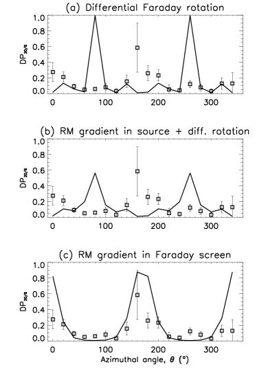
Figure 8: Observed (squares with error bars) and expected (solid line) depolarization between $\lambda 20\,{\rm cm}$ and $\lambda 6\,{\rm cm}$, $\mathrm{DP}_{20/6}$, for the ring $10<r<12\,{\rm kpc}$ assuming various depolarization mechanisms. The azimuthal angle $\theta$ is measured counterclockwise from the northern major axis. Depolarization due to (a) differential Faraday rotation using Eq. (13), (b) RM gradients in the synchrotron source and differential Faraday rotation from Eq. (16) and (c) RM gradients in a Faraday screen given by Eq. (17) are represented by solid lines. RM and the gradient in RM are derived from the fitted magnetic field described in Sect. 5. We conclude that foreground RM gradients, illustrated in panel (c), dominate other wavelength dependent depolarization mechanisms.

Can we recognize the signature of any of the depolarization mechanisms discussed in Appendix A in the observations? Before considering a model based on a combination of effects it is instructive to consider each of these mechanisms separately.

The effect of wavelength independent depolarization is removed by considering Eq. (6). By comparing the ratio of the observed degrees of polarization at $\lambda 20\,{\rm cm}$ and $\lambda 6\,{\rm cm}$, $\mathrm{DP}_{20/6}=P_{20}/P_{6}$, with that expected from Eqs. (13) to (17), we identify which wavelength dependent depolarization mechanisms are dominant.

The observed $\mathrm{DP}_{20/6}$, plotted in Fig. 8, has a marked azimuthal variation with strong depolarization at $\lambda 20\,{\rm cm}$ near the minor axis ($\theta=90\degr$ and $270\degr$, where $\mathrm{DP}_{20/6}\simeq 0.1$) and less depolarization on the major axis ($\theta=0\degr$ and $180\degr$ where $\mathrm{DP}_{20/6}\geq 0.4$). Note that the observed $\mathrm{DP}_{20/6}(\theta)$ is roughly proportional to the derivative of RM$(\theta)$ (Fig. 7).

Gradients in the foreground RM due to magnetic fields in the Milky Way, $\,\mathrm{RM_{fg}}$, in the direction of M 31, are weak (Han et al. Han98 (1998)) and unlikely to cause the observed variation of RM and DP with azimuth in M 31. Thus, depolarization must occur within M 31. For the rest of the analysis of depolarization we consider the RM intrinsic to M 31, $\,\mathrm{RM_{i}}=\,\mathrm{RM}-\,\mathrm{RM_{fg}}$.

The smooth, sinusoidal azimuthal variation of RM (Fig. 7a) can be completely accounted for by an azimuthal variation of $\,B_{\parallel}$ deduced in Sect. 5, indicating that $\langle n_{\mathrm{e}}\rangle L$ is indeed roughly constant in azimuth. The turbulent magnetic field, $\,b$, derived using the equipartition approach described in Sect. 3, is also constant in azimuth for each ring. Therefore the dispersion in RM, $\sigma_{\mathrm{RM}}$, and hence depolarization due to Faraday dispersion, is roughly constant at a given radius, and the azimuthal variation in $\mathrm{DP}_{20/6}$ cannot be explained by Faraday dispersion [Eqs. (14) and (15)]. This does not mean that Faraday dispersion is ineffective in M 31, but rather that the strong azimuthal pattern in $\mathrm{DP}_{20/6}$ cannot be explained by this mechanism.

The remaining wavelength dependent depolarizing mechanisms are all caused by the regular magnetic field: differential Faraday rotation, RM gradients within the emitting layer, and RM gradients in a foreground Faraday screen. The first two effects are unavoidable while the third effect requires the existence of a ’thick disk’ of magnetic fields and thermal gas invisible in synchrotron emission. Differential Faraday rotation in the source is strongest near the major axis where the line-of-sight magnetic field $\,B_{\parallel}$ is maximum, resulting in a depolarization pattern very different from that observed (Fig. 8a). The azimuthal gradient in $\,B_{\parallel}$ is also maximum near the minor axis (where it changes sign). Therefore, depolarization due to gradients in RM in the synchrotron source is strong near the minor axis and weak near the major axis, but still does not overcome the differential Faraday rotation that produces a different pattern (Fig. 8b). On the other hand a foreground Faraday screen does not produce any differential Faraday rotation, and so depolarization due to the RM gradients in a foreground screen is dominant, producing a correct pattern shown in Fig. 8c.

Thus, the global pattern of the azimuthal variation of $\mathrm{DP}_{20/6}$ can only be reproduced by depolarization due to RM gradients in a Faraday screen (the bottom frame of Fig. 8). This mechanism must be the dominant cause of the azimuthal pattern in wavelength dependent depolarization. This is true in the whole radial range $6\leq r\leq 14\,{\rm kpc}$. Berkhuijsen et al. (Berkhuijsen03 (2003)) found that contours of RM and $\mathrm{DP}_{11/6}$ are often perpendicular to each other where they cross (see their Fig. 14) and noted that this suggests RM gradients as an important cause of depolarization. Earlier, Berkhuijsen & Beck (Berkhuijsen90 (1990)) found that RM gradients were primarily responsible for depolarization in the southwestern quadrant of M 31 and Horellou et al. (Horellou92 (1992)) observed that contours of $\mathrm{DP}$ and RM are perpendicular at crossing points for the galaxy M 51.

The minima in $\mathrm{DP}_{20/6}$ produced by the Faraday screen are noticeably deeper than those observed (at $\theta\approx 90\degr$ and $270\degr$ in Fig. 8c). As discussed in Sect. 6.2, this can be explained by other, less important depolarization mechanisms.

6.2 The thermal and synchrotron disk scale heights

Figure 9: Observed (squares with error bars) and expected (solid line) depolarization between $\lambda 20\,{\rm cm}$ and $\lambda 6\,{\rm cm}$, $\mathrm{DP}_{20/6}$, due to RM gradients and differential Faraday rotation using Eqs. (7), (11) and (12), for the ring $10<r<12\,{\rm kpc}$ and with different ratios of the synchrotron to thermal disk scale heights, $q=h_{\mathrm{syn}}/h_{\mathrm{th}}$.

We have identified RM gradients in a Faraday screen as the dominant depolarizing mechanism responsible for the observed azimuthal pattern of $\mathrm{DP}_{20/6}$ in M 31. The fit to observations in Fig. 8c can be improved by including other depolarizing effects, especially Faraday dispersion. Also, the effectiveness of the Faraday screen depends upon its relative thickness, compared to that of the synchrotron emitting layer. Now we attempt to recover information about the relative heights of the emitting and Faraday rotating layers from fitting the depolarization.

A full description of depolarization due to the regular magnetic field (i.e., differential Faraday rotation, RM gradients inside the synchrotron emitting layer and in a Faraday screen) is given by the product of Eqs. (16) and (17). The intrinsic Faraday rotation measure $\,\mathrm{RM_{i}}$ and its increment $\Delta\,\mathrm{RM}$ across each sector can be calculated from the fits for the regular magnetic field discussed in Sect. 5. We split $\,\mathrm{RM_{i}}$ into two components, $\,\mathrm{RM}_{\mathrm{d}}$ arising within the synchrotron disk and $\,\mathrm{RM}_{\mathrm{s}}$ arising in the part of the thermal layer above the synchrotron disk (see Fig. 10); the scale height of the synchrotron layer is taken from Sect. 3.1. The first component will produce depolarization due to differential Faraday rotation, but the latter will only contribute to Faraday screen effects. The gradient in $\,\mathrm{RM_{i}}$ is similarly split into $\Delta\,\mathrm{RM}_{\mathrm{d}}$ and $\Delta\,\mathrm{RM}_{\mathrm{s}}$. In terms of these variables, the degree of polarization with allowance for Faraday dispersion, differential Faraday rotation and rotation measure gradients in both the thermal disk and Faraday screen is given by

$$P(\lambda)=P_{0}P_{\mathrm{in}}(\lambda)P_{\mathrm{ex}}(\lambda)\left|\exp\left[2i{\,\mathrm{RM}_{0}}_{\mathrm{s}}\lambda^{2}\!-\!2\left(\Delta\,\mathrm{RM}_{\mathrm{s}}\lambda^{2}\right)^{2}\right]\phantom{int_{0}^{1}}\right.$$

$$\left.\mbox{}\qquad\quad\times\int_{0}^{1}\exp(4i{\,\mathrm{RM}_{0}}_{\mathrm{d}}\lambda^{2}s)\frac{\sin(2\Delta\,\mathrm{RM}_{\mathrm{d}}\lambda^{2}s)}{2\Delta\,\mathrm{RM}_{\mathrm{d}}\lambda^{2}s}\,ds\right|,$$ (7)

where subscript zero refers to a value at the sector centre. We can reasonably assume that depolarization due to Faraday dispersion in the emitting layer is much stronger than Faraday dispersion in the foreground screen (turbulent magnetic fields and thermal gas density will be stronger near the mid-plane) and so $P_{\mathrm{in}}P_{\mathrm{ex}}\sim P_{\mathrm{in}}$.

Figure 10: Sketch showing the scale heights of the thermal disk, $h_{\mathrm{th}}$, synchrotron disk, $h_{\mathrm{syn}}$, and the depth in the thermal disk from which polarized emission is visible at $\lambda 20\,{\rm cm}$, $\Delta z$. The galactic midplane is at $z=0$, i.e., at the bottom of the figure. The deeper layers of the synchrotron disk are invisible in polarized emission because of internal Faraday dispersion. This sketch is only an illustration: note that $\Delta z$ can exceed $h_{\mathrm{th}}$ if more than half the disk thickness is visible. However, $h_{\mathrm{th}}-h_{\mathrm{syn}}\leq\Delta z\leq h_{\mathrm{th}}+h_{\mathrm{syn}}$ with the extreme values corresponding to $\mathrm{DP}_{20/6}=0$ and 1, respectively.

Since the galactic disk may be opaque to polarized emission at longer wavelengths, mainly due to internal Faraday dispersion, the effective path length can differ from that suggested by the disk scale height (c.f. Sokoloff et al. Sokoloff98 (1998), Berkhuijsen et al. Berkhuijsen97 (1997)). We use the ‘opaque layer’ approximation of Sokoloff et al. (Sokoloff98 (1998), Sect. 6.3) to describe the visible depth $\Delta z$ in terms of the depolarization due to internal Faraday dispersion assuming that all the observed polarized emission at $\lambda 20\,{\rm cm}$ arises from an upper layer in the synchrotron disk. Figure 10 shows how $h_{\mathrm{th}}$, $h_{\mathrm{syn}}$ and $\Delta z$ are related. The path lengths over which the observed polarized emission is produced are $\Delta z-(h_{\mathrm{th}}-h_{\mathrm{syn}})$ at $\lambda 20\,{\rm cm}$ (here $\Delta z$ is a function of $\lambda$) and $2h_{\mathrm{syn}}$ at $\lambda 6\,{\rm cm}$, where the disk is assumed to be transparent to polarized emission. Then a crude estimate of $\Delta z$ in terms of the observed degrees of polarization follows from assuming that depolarization due to internal Faraday dispersion is constant for all sectors in a ring:

$$\Delta z=h_{\mathrm{th}}+h_{\mathrm{syn}}\left(2\,DP_{\mathrm{in}}-1\right)\;,$$ (8)

where $DP_{\mathrm{in}}=P_{\mathrm{in}}(20\,{\rm cm})/P_{\mathrm{in}}(6\,{\rm cm})$ is depolarization due to internal Faraday dispersion alone (see Sect. 3.3.3 in Berkhuijsen et al. Berkhuijsen97 (1997)). Since some depolarization due to other mechanisms occurs within $\Delta z$, this yields minimum values for the thickness of the visible layer. Equation (8) then gives the parameter $\xi_{\lambda}$ in Eq. (4), in terms of $q=h_{\mathrm{syn}}/h_{\mathrm{th}}$ and $DP_{\mathrm{in}}$, via (Berkhuijsen et al. Berkhuijsen97 (1997))

$$\xi_{\lambda}=\frac{1}{2}\left(1+\frac{\Delta z-h_{\mathrm{syn}}}{h_{\mathrm{th}}}\right),$$ (9)

so we have

$$\xi_{\lambda}=1+q(DP_{\mathrm{in}}-1).$$ (10)

The parameter $\xi_{\lambda}$ links the modelled regular magnetic field described in Sect. 5, from which we obtain $\,\mathrm{RM}$ and $\Delta\,\mathrm{RM}$, and the model for Faraday depolarization described in this section. Our aim is to obtain satisfactory fits for both models using the same $\xi_{\lambda}$ in each.

For a thermal layer thicker than the synchrotron disk (the configuration that produces a foreground Faraday screen), $\Delta z\geq h_{\mathrm{th}}-h_{\mathrm{syn}}$, Berkhuijsen et al. (Berkhuijsen97 (1997)) showed that

$${\,\mathrm{RM}_{0}}_{\mathrm{d}} = {\textstyle\frac{1}{2}}\,\mathrm{RM}_{0}\frac{\Delta z-(h_{\mathrm{th}}-h_{\mathrm{syn}})}{h_{\mathrm{th}}}=q\,\mathrm{RM}_{0}\,DP_{\mathrm{in}},$$ (11)

$${\,\mathrm{RM}_{0}}_{\mathrm{s}} = \,\mathrm{RM}_{0}\frac{h_{\mathrm{th}}-h_{\mathrm{syn}}}{h_{\mathrm{th}}}=(1-q)\,\,\mathrm{RM}_{0},$$ (12)

where the final equalities result from substitution of Eq. (8). Using Eqs. (11) and (12) we can express $P(\lambda)$ in Eq. (7) as a function of $q=h_{\mathrm{syn}}/h_{\mathrm{th}}$, the ratio of the scale heights of the synchrotron and thermal disks, and $DP_{\mathrm{in}}$. We fit the values of $q$ and $DP_{\mathrm{in}}$ by comparing $\mathrm{DP}_{20/6}$ obtained from Eq. (7) to the observed values in each sector. Figure 9 compares the calculated $\mathrm{DP}_{20/6}$, for $q$ between $0.1$ and $0.4$, with observed values in the ring 10–12 kpc, and shows how increasing the relative scale height of the synchrotron disk reduces the effect of the Faraday screen and enhances depolarization due to differential Faraday rotation, which is strongest on the major axis.

Figure 11: Observed (squares with error bars representing $1\sigma$ error) and expected (solid line) depolarization between $\lambda 20\,{\rm cm}$ and $\lambda 6\,{\rm cm}$, $\mathrm{DP}_{20/6}$, due to Faraday effects using Eq. (7), (11) and (12), for each of four radial rings. The expected depolarization is fitted by varying the ratio of the synchrotron to thermal disk scale heights, $q=h_{\mathrm{syn}}/h_{\mathrm{th}}$ and depolarization due to internal Faraday dispersion, $DP_{\mathrm{in}}$. The fitted values of $q$ are $0.6$, $0.6$, $0.4$, and $0.3$ and of $DP_{\mathrm{in}}$ $0.1$, $0.1$, $0.3$ and $0.2$ in panels (a), (b), (c) and (d), respectively. The solid line was obtained using RM derived from the regular magnetic field fits of Table LABEL:tab:results.

Table 3: Parameters derived from the model of Faraday depolarization and their $2\sigma$ errors.

Ring (kpc)	$q=h_{\mathrm{syn}}/h_{\mathrm{th}}$	$DP_{\mathrm{in}}$	$h_{\mathrm{th}}$ (kpc)
6–8	No statistically good fit found
8–10	$0.6\pm 0.1$	$0.1\pm 0.1$	$0.55\pm 0.10$
10–12	$0.4^{+0.4}_{-0.2}$	$0.3^{+0.7}_{-0.1}$	$0.90^{+0.90}_{-0.45}$
12–14	$0.3^{+0.5}_{-0.3}$	$0.2\pm 0.2$	$1.3^{+2.6}_{-0.8}$

Figure 11 shows the azimuthal variation of the depolarization for the best fitting $q$ for each ring. The fitted values of $q=h_{\mathrm{syn}}/h_{\mathrm{th}}$ and $DP_{\mathrm{in}}$ are given in Table LABEL:tab:dp, where the quoted $2\sigma$ errors represent the extent of the $(q,DP_{\mathrm{in}})$-parameter space within the relevant $\chi^{2}$ contour. These errors are large, but it is remarkable that we can successfully model Faraday depolarization in such a complex system using such a simple, two parameter model. Despite the uncertainty in the precise values of the model parameters, the key result of this section is robust; the strong azimuthal pattern of depolarization can only be explained by a Faraday screen acting within M 31 and hence the thermal electron layer must be significantly thicker than the synchrotron emitting layer.

For $8<r<14\,{\rm kpc}$ the modelled $\mathrm{DP}_{20/6}$ reproduce the observations well. For each of these rings the fitted $\mathrm{DP}_{20/6}$ meets the $\chi^{2}$ test for statistical significance at the $2\sigma$ level. In the two rings at largest radii the results of the depolarization modelling are fully consistent with the polarization angle model used to deduce the regular magnetic field structure in Sect. 5. The two models are linked by the parameter $\xi_{\lambda}$ – a weighting for the depth in the emission layer visible at long wavelengths – in Eqs. (4) and (10). For the rings 10–12 kpc and 12–14 kpc, $q$ and $DP_{\mathrm{in}}$ in Table LABEL:tab:dp give $\xi_{20}=0.7\pm{0.3}$ and $\xi_{20}=0.8^{+0.2}$, respectively. In Sect. 5 we adopted $\xi_{20}=0.75$ for all of the rings and discrepancies of order $\pm 0.1$ have a negligible effect on the fitted magnetic field parameters given in Table LABEL:tab:results.

For the ring 8–10 kpc, $q$ and $DP_{\mathrm{in}}$ give $\xi_{20}=0.5\pm 0.2$, whereas the best fit to the polarization angles in Table LABEL:tab:results requires $\xi_{20}=0.75$. We can achieve self consistency between the magnetic field and depolarization models by discarding more measured polarization angles in Sect. 5, i.e. by making the model of the magnetic field worse. However, the main problem with the depolarization model in this ring is that around the north end of the major axis our method of averaging the data gives zero average polarized emission at $\lambda 20\,{\rm cm}$ in three sectors. (The polarized intensity is averaged from maps smoothed to $3\arcmin$ resolution; the polarization angles are derived from $45\arcsec$ maps at $\lambda 20\,{\rm cm}$ and do not suffer from this problem.) Without measurements at both ends of the major axis the fitted $\mathrm{DP}_{20/6}$ favours a model with stronger Faraday dispersion i.e. a model that has a less prominent double minimum. For these reasons we prefer to retain the magnetic field model obtained with $\xi=0.75$ – to keep $\xi_{20}$ the same for each ring – and accept that the depolarization model for this ring is poorer than for 10–12 kpc and 12–14 kpc.

The quality of the fit is clearly bad in the ring 6–8 kpc (Fig. 11a) where the magnetic field, deduced in Sect. 5, contains both the axisymmetric ($m=0$) and the quadrisymmetric ($m=2$) components as given in Table LABEL:tab:results. In Sect. 5.2.1 we show that this ring may have a more complicated regular magnetic field structure than the purely azimuthal fields in the other rings. The modelled azimuthal patterns of RM and the gradient in RM are rather complicated in the ring 6–8 kpc and no good fit can be obtained. The results would be better if we used a simpler fit involving a purely axisymmetric magnetic field. However, as explained in Sect. 5.2.1, nine polarization angle measurements must be discarded to make an $m=0$ magnetic field model, and the consequent degrading of the regular magnetic field model is not justified.

Using $h_{\mathrm{syn}}$, at $\lambda 20\,{\rm cm}$, from Table 1, we can estimate $h_{\mathrm{th}}$ from the fitted values for $q=h_{\mathrm{syn}}/h_{\mathrm{th}}$. The results are shown in Table LABEL:tab:dp. These scale heights are about a factor of two or more greater than previously expected in M 31, where the low star formation rate and absence of a radio halo were thought to imply the likely absence of a thick ionized disk (Walterbos & Braun Walterbos94 (1994)).

We emphasize that the gradients in rotation measure producing most of the depolarization in M 31 are due to the highly axisymmetric regular magnetic field that we find from an analysis of polarization angles in Sect. 5. For simplicity, in modelling the depolarization we assumed that the regular magnetic field has the same configuration and strength throughout the full vertical extent of the thermal layer (including the synchrotron emitting disk). If the regular magnetic field strength or the thermal electron density has a maximum above the emitting disk (i.e., at $z\gtrsim 300\,{\rm pc}$), the RM required to produce the observed depolarization can be generated in a thinner layer and $h_{\mathrm{th}}$ will be lower than estimated above, but still $h_{\mathrm{th}}>h_{\mathrm{syn}}$.

In Sect. 2.2.2 the limitations of the $\lambda 20\,{\rm cm}$ polarization data when smoothed to $3\arcmin$ were discussed; foreground emission from the Milky Way cannot be subtracted from the emission from M 31 and so the $\lambda 20\,{\rm cm}$ polarized intensities are upper limits. The values of $q=h_{\mathrm{syn}}/h_{\mathrm{th}}$ and $DP_{\mathrm{in}}$ shown in Table LABEL:tab:dp were derived assuming that all of the polarized emission at $\lambda 20\,{\rm cm}$ comes from M 31 and so are upper limits on $q$ and $DP_{\mathrm{in}}$.

The corresponding lower limits (i.e., giving depolarization stronger than required) can be obtained assuming that the emission from M 31 is nearly completely depolarized at $\lambda 20\,{\rm cm}$. Without Faraday depolarization, the $\lambda 20\,{\rm cm}$ polarized emission from M 31 will have the same azimuthal pattern as the $\lambda 6\,{\rm cm}$ $PI$ shown in Fig. 7(c). Total depolarization ($\mathrm{DP}_{20/6}=0$) will occur when $DP_{\mathrm{in}}$ and differential rotation are just strong enough to depolarize the emission on the major axis ($\theta=0\degr,180\degr$) and RM gradients are just sufficient to depolarize emission from the minor axis ($\theta=90\degr,270\degr$). From Fig. 9(a) we estimate that, for the ring 10$<r<$12 kpc, complete depolarization will occur if $q\simeq 0.1$ and $DP_{\mathrm{in}}\simeq 0.1$. These are the lower limits on $q$ and $DP_{\mathrm{in}}$.

The regular magnetic field must be coherent in $z$ over at least the scale height of the thermal disk, and we have shown that the latter must exceed that of the synchrotron disc. This poses the intriguing question of why the cosmic rays in M 31 are confined to a layer several times thinner than the regular magnetic field. One possible answer relies on the usual assumption of equipartition between the cosmic ray and magnetic field energy densities. Then the synchrotron emissivity depends upon the fourth power of the magnetic field and so $h_{B}\sim 4h_{syn}\simeq 1.5\,{\rm kpc}$. This scale height is in good agreement with $h_{\mathrm{th}}$ derived from our analysis of depolarization (at least for the two rings with the most reliable model of $\mathrm{DP}_{20/6}$). In M 31, the magnetic field is well ordered with $\,B\simeq\,b$ and there is no significant vertical component of the magnetic field (see Sect. 5). This may be sufficient to suppress diffusion of cosmic rays perpendicular to the disk plane and so constrain them to the same layer as their sources.

6.3 Thermal electron densities

Using Eq. (3) and the equipartition regular magnetic field strengths given in Table 1, the rotation measures from Table LABEL:tab:results and the thermal disk scale heights of Table LABEL:tab:dp we can derive average thermal electron densities for M 31 in the radial range $8<r<14\,{\rm kpc}$. This gives $\langle n_{\mathrm{e}}\rangle\simeq 0.008,0.007$ and $0.004\,{\rm cm^{-3}}$ for the rings 8–10, 10–12 and 12–14 kpc, respectively. These values refer to the upper layers of the thermal electron layer, $z\ga h_{\mathrm{syn}}\simeq 200$–300 pc, that act as the Faraday screen.

Electron density closer to the midplane can be obtained from the amount of depolarization due to Faraday dispersion between $\lambda 20\,{\rm cm}$ and $\lambda 6\,{\rm cm}$, $DP_{\mathrm{in}}\simeq 0.1$ as obtained above. Using Eq. (14) with $b=5\,\mu{\rm G}$, $L=200\,{\rm pc}$ and $d=50\,{\rm pc}$, we obtain $\sigma_{\mathrm{RM}}\simeq 550\left(\langle n_{\mathrm{e}}^{2}\rangle^{1/2}/1\,{\rm cm^{-3}}\right)\,{\rm rad\,m^{-2}}$ and then $DP_{\mathrm{in}}=0.1$ corresponds to $n_{\mathrm{e}}\simeq 0.1\,{\rm cm^{-3}}$. This estimate is compatible with that obtained by Walterbos & Braun (Walterbos94 (1994)) from H $\alpha$ emission measures of the diffuse ionised gas, $\langle n_{\mathrm{e}}\rangle\simeq 0.08$–$0.04\,{\rm cm^{-3}}$ with a filling factor 0.2.

Thus, the equipartition magnetic field strength, rotation measures and the scale heights of the thermal disk derived in our models produce an estimate for $\langle n_{\mathrm{e}}\rangle$ that is in broad agreement with $\langle n_{\mathrm{e}}\rangle$ obtained from completely different data and methods.

Berkhuijsen et al. (Berkhuijsen03 (2003)) note that there is little correlation between RM and thermal emission in M 31 and suggest that the small filling factor of H ii regions may be the reason. This is consistent with our conclusion that much of the Faraday rotation in M 31 is produced in a Faraday screen.

6.4 Review of the method

In fitting the modelled to observed polarization angles in Sect. 5, we use the parameter $\xi_{\lambda}$ to account for the partial opacity of the galaxy’s disk to polarized emission at $\lambda 20\,{\rm cm}$. In order to estimate $\xi_{\lambda}$ we need to know the ratio of the scale heights of the synchrotron and thermal disks, $q=h_{\mathrm{syn}}/h_{\mathrm{th}}$, but the values for $q$ deduced in Sect. 6.2 make use of RM calculated from the fits of Sect. 5. We used an iterative approach to try to obtain a model consistent with both the observed depolarization and polarization angles. This method was successful for the two outer rings, after one iteration, but not for the rings 6–8 kpc and 8–10 kpc. For these rings we adopted $\xi=0.75$ from the self-consistent models of the rings 10–12 kpc and 12–14 kpc.

7 Summary

Sensitive, high resolution, multi-wavelength radio polarization observations have been used to study the magnetic field of M 31, between the radii of $6$ and $14\,{\rm kpc}$. The powerful method of using polarization angles to uncover the regular magnetic field structure was supplemented by a systematic analysis of depolarization to produce a model of the regular magnetic field which is consistent with all of the radio polarization data for $10<r<14\,{\rm kpc}$.

Our main conclusions are as follows :

1. The regular magnetic field in M 31 is axisymmetric to a very good approximation.

2. The magnetic field has a significant radial component at all radii and so is definitely not purely azimuthal. Vector lines of the regular magnetic field in the radial range $6\lesssim r\lesssim 10\,{\rm kpc}$ can be approximated by trailing logarithmic spirals, with the pitch angle $p\simeq-16\degr$. The magnetic spiral becomes tighter at large radii, with $|p|$ decreasing to $p\simeq-7\degr$ at $r=12$–$14\,{\rm kpc}$. The magnitude and trend of magnetic pitch angles is in broad agreement with those expected from dynamo theory (Shukurov Shukurov00 (2000)).

3. Analysis of the azimuthal pattern of the wavelength dependent depolarization reveals that a Faraday active screen lies above the synchrotron emitting disk of M 31. The diffuse thermal disk is thicker than previously expected, with a scale height of $h_{\mathrm{th}}\sim 1\,{\rm kpc}$.

4. The scale height of the regular magnetic field is at least equal to $h_{\mathrm{th}}$.

5. The magnetic field in M 31 extends inside and outside of $r\simeq 10\,{\rm kpc}$, as found by Han et al. (Han98 (1998)), and does not have a strong maximum at this radius. The bright radio ring is a result of a high density of cosmic ray electrons.

6. The equipartition field strengths are about 5$\,\mu{\rm G}$ for both the regular and turbulent field components, without significant variation between 6 kpc and 14 kpc radius.

7. Faraday rotation measures and equipartition field strengths are in agreement for average electron densities of 0.008–0.004$\,{\rm cm^{-3}}$. The electron densities inferred from the Faraday dispersion measures are $\simeq 0.1\,{\rm cm^{-3}}$, close to the average electron densities found by Walterbos & Braun (Walterbos94 (1994)). This suggests that the diffuse ionised gas is mainly responsible for the Faraday rotation, with little contribution to RM from H ii regions.

Our analysis of depolarization in M 31 is the most extensive undertaken to date for a spiral galaxy, and shows that the theory of radio depolarization developed by Burn (Burn66 (1966)) and Sokoloff et al. (Sokoloff98 (1998)) can be used not only to identify the causes of depolarization, but also to reveal properties of the diffuse ISM in external galaxies.

Appendix A Depolarization mechanisms

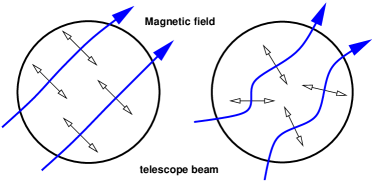
Figure 12: Sketch showing wavelength independent depolarization. The double headed arrows represent E-vectors.

Wavelength independent depolarization is caused by tangling of magnetic field lines in the emitting region (Figure 12). The intrinsic polarization angle of synchrotron radiation is perpendicular to the local magnetic field orientation and so tangled magnetic field lines result in emission at a range of polarization angles within a single telescope beam. As long as the beam sizes are equal, the degree of depolarization due to tangled magnetic field lines will be the same at all wavelengths.

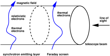
Figure 13: Sketch of synchrotron emitting layer and a foreground Faraday screen.

Faraday rotation by both regular and turbulent magnetic fields results in wavelength dependent depolarization. It is useful to consider separately Faraday effects within the synchrotron emitting layer and Faraday rotation in regions where there is no emission, i.e. within a Faraday screen (Figure 13).

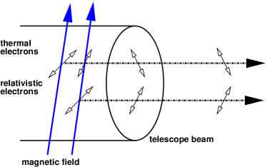
Figure 14: Differential Faraday rotation occurs within the synchrotron emitting layer. Emission from different depths along the same line of sight undergoes different amounts of Faraday rotation, causing depolarization. For clarity the sketch separates emission from different depths.

The regular field in the synchrotron emitting layer causes depolarization by differential Faraday rotation, whereby polarized emission from different depths along the line of sight is rotated by different amounts (Figure 14). In a slab with uniform magnetic field and electron density the degree of polarization is (Burn Burn66 (1966), Sokoloff et al. Sokoloff98 (1998))

$$P_{\mathrm{reg}}=P_{0}\left|\frac{\sin(2\,\mathrm{RM}\lambda^{2})}{2\,\mathrm{RM}\lambda^{2}}\right|,$$ (13)

where $\,\mathrm{RM}=0.81\langle n_{\mathrm{e}}\rangle\,B_{\parallel}L/2$ is the observed rotation measure in units of $\!\,{\rm rad\,m^{-2}}$, with $\langle n_{\mathrm{e}}\rangle$ the average thermal electron density in $\!\,{\rm cm^{-3}}$, $\,B_{\parallel}$ the component of $\,B$ parallel to the line of sight in $\,\mu{\rm G}$ and $L$ the path length through the Faraday active emitting layer, in $\!\,{\rm pc}$.

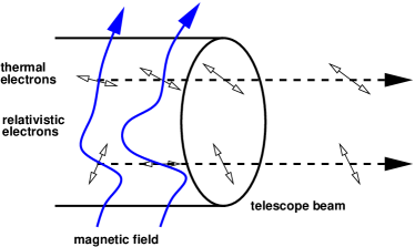
Figure 15: Sketch illustrating Faraday dispersion. When this effect occurs within the synchrotron emitting layer it is called internal Faraday dispersion; occurrence in a Faraday screen (no synchrotron emission) is external Faraday dispersion. Note that the required variation of rotation measure within the beam could also be caused by fluctuations of thermal electron density. In that case the magnetic field could be totally regular but Faraday dispersion would still occur.

The presence of unresolved, turbulent magnetic field means that polarized emission along different lines of sight within the telescope beam undergoes different amounts of Faraday rotation (Figure 15). When the emitting and rotating layers coincide, the effect is called internal Faraday dispersion, and the degree of polarization is given by Sokoloff et al. (Sokoloff98 (1998)) as

$$P_{\mathrm{in}}=P_{0}\frac{1-\exp(-2\sigma_{\mathrm{RM}}^{2}\lambda^{4})}{2\sigma_{\mathrm{RM}}^{2}\lambda^{4}},$$ (14)

where $\sigma_{\mathrm{RM}}^{2}=0.81\langle n_{\mathrm{e}}\,b\rangle^{2}2Ld$ with $d$ the correlation scale (half the turbulent cell size) of the turbulent magnetic field in parsecs. Burn (Burn66 (1966)) gives the depolarization due to external Faraday dispersion (due to turbulent fields in front of the synchrotron source) as

$$P_{\mathrm{ex}}=P_{0}\exp(-2\sigma_{\mathrm{RM}}^{2}\lambda^{4}).$$ (15)

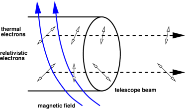
Figure 16: Depolarization due to gradients in rotation measure: if RM varies across the beam, different parts of the beam area contribute with different polarization angles. Note that variations of thermal electron density or magnetic field strength can also produce RM gradients even in a totally regular magnetic field.

Gradients in rotation measure across the beam cause depolarization that is especially strong when the resolution of observations is low (Figure 16). For depolarization by RM gradients within the synchrotron source, including the effect of differential Faraday rotation, Sokoloff et al. (Sokoloff98 (1998)) obtained

$$P_{\mathrm{\Delta in}}=P_{0}\left|\int_{0}^{1}\exp(4i\,\mathrm{RM_{0}}\,\lambda^{2}s)\frac{\sin(2\,\Delta\,\mathrm{RM}\,\lambda^{2}s)}{2\,\Delta\,\mathrm{RM}\,\lambda^{2}s}\,ds\right|,$$ (16)

where $\mathrm{RM_{0}}$ is $\,\mathrm{RM}$ at the centre of the beam, $\Delta\,\mathrm{RM}$ is the increment in $\,\mathrm{RM}$ across the beam and the normalized integration variable $s$ describes the line of sight within the synchrotron disk, $0\leq s\leq 1$. Equation (16) holds for both resolved and unresolved RM gradients (Sokoloff et al. Sokoloff98 (1998)). Depolarization by a resolved RM gradient in a Faraday screen is given by Sokoloff et al. (Sokoloff98 (1998)) as

$$P_{\mathrm{\Delta ex}}=P_{0}\left|\exp\left[2i\,\mathrm{RM_{0}}\,\lambda^{2}-2\left(\Delta\,\mathrm{RM}\,\lambda^{2}\right)^{2}\right]\right|.$$ (17)

References

- (1) Beck, R. 1982, A&A, 106, 121
- (2) Beck, R. 2000, in The Interstellar Medium in M 31 and M 33, Proc. 232 WE-Heraeus Seminar, ed. E.M. Berkhuijsen, R. Beck, & R.A.M. Walterbos (Aachen: Shaker), 173
- (3) Beck, R., Berkhuijsen, E.M., & Wielebinski, R. 1978, A&A, 68, L27
- (4) Beck, R., Loiseau, N., Hummel, E., et al. 1989, A&A, 222, 58
- (5) Beck, R., Brandenburg, A., Moss, D., Shukurov, A., & Sokoloff, D. 1996, ARA&A, 34, 155
- (6) Beck, R., Berkhuijsen, E.M., & Hoernes, P. 1998, A&AS, 129, 329
- (7) Berkhuijsen, E.M. 1977, A&A, 57, 9
- (8) Berkhuijsen, E.M., & Wielebinski, R. 1974, A&A, 34, 173
- (9) Berkhuijsen, E.M., & Beck, R. 1990, in Galactic and Intergalactic Magnetic Fields, ed. R. Beck, P.P. Kronberg, & R. Wielebinski (Dordrecht: Kluwer), IAU Symp., 140, 201
- (10) Berkhuijsen, E.M., Golla, G., & Beck, R. 1991, in The Interstellar Disk–Halo Connection in Galaxies, Proc. IAU Symp. 144, ed. H. Bloemen (Dordrecht: Kluwer), 233
- (11) Berkhuijsen, E.M., Bajaja, E., & Beck, R. 1993, A&A, 279, 359
- (12) Berkhuijsen, E.M., Horellou, C., Krause, M., et al. 1997, A&A, 318, 700
- (13) Berkhuijsen, E.M., Nieten, Ch., & Haas, M. 2000, in The Interstellar Medium in M 31 and M 33, Proc. 232 WE-Heraeus Seminar, ed. E.M. Berkhuijsen, R. Beck, & R.A.M. Walterbos (Aachen: Shaker), 187
- (14) Berkhuijsen, E.M., Beck, R., & Hoernes, P. 2003, A&A, 398, 937
- (15) Braun, R. 1991, ApJ, 372, 54
- (16) Burn, B.J. 1966, MNRAS, 133, 67
- (17) Fletcher, A., Beck, R., Berkhuijsen, E.M. & Shukurov, A. 2000 in The Interstellar Medium in M 31 and M 33, Proc. 232 WE-Heraeus Seminar, ed. E.M. Berkhuijsen, R. Beck, & R.A.M. Walterbos (Aachen: Shaker), 201
- (18) Gräve, R., Emerson, D.T. & Wielebinski, R. 1981, A&A, 98, 260
- (19) Guélin, M., Nieten, C., Neininger, N., Muller, S., Lucas, R., Ungerechts, H., & Wielebinski, R. 2000, in The Interstellar Medium in M 31 and M 33, Proc. 232 WE-Heraeus Seminar, ed. E.M. Berkhuijsen, R. Beck, & R.A.M. Walterbos (Aachen: Shaker), 15
- (20) Han, J.L., Beck, R., & Berkhuijsen, E.M. 1998, A&A, 335, 1117
- (21) Horellou, C., Beck, R., Berkhuijsen, E.M., Krause, M., & Klein, U. 1992, A&A, 265, 417
- (22) Hummel, E., Dahlem, M., van der Hulst, J.M., & Sukumar, S. 1991, A&A, 246, 10
- (23) Longair, M. 1994, High Energy Astrophysics Volume 2 (Cambridge University Press)
- (24) Moss, D., Shukurov, A., Sokoloff, D.D., Berkhuijsen, E.M., & Beck, R. 1998, A&A, 335, 500
- (25) Pacholczyk, A.G. 1970, Radio Astrophysics (San Francisco: Freeman)
- (26) Pooley, G.G. 1969, MNRAS, 144, 101
- (27) Reynolds, R.J. 1991, in The Interstellar Disk–Halo Connection in Galaxies, Proc. IAU Symp. 144, ed. H. Bloemen (Dordrecht: Kluwer), 67
- (28) Ruzmaikin, A., Sokoloff, D., Shukurov, A., & Beck R. 1990, A&A, 230, 284
- (29) Shukurov, A. 2000 in The Interstellar Medium in M 31 and M 33, Proc. 232 WE-Heraeus Seminar, ed. E.M. Berkhuijsen, R. Beck, & R.A.M. Walterbos (Aachen: Shaker), 191
- (30) Shukurov, A., & Berkhuijsen, E.M. 2003, MNRAS, 342, 496
- (31) Sofue, Y., & Beck, R. 1987, PASJ, 39, 541
- (32) Sokoloff, D., Shukurov, A., & Krause, M. 1992, A&A, 264, 396
- (33) Sokoloff, D.D., Bykov, A.A., Shukurov, A., et al. 1998, MNRAS, 299, 189; 1999, MNRAS, 303, 207
- (34) Walterbos, R.A.M., & Braun, R. 1994, ApJ, 431, 156
- (35) Wardle, J.F.C., & Kronberg, P.P. 1974, ApJ, 194, 249