Cold Atom Clocks, Precision Oscillators and Fundamental Tests

Abstract

We describe two experimental tests of the Equivalence Principle that are based on frequency measurements between precision oscillators and/or highly accurate atomic frequency standards. Based on comparisons between the hyperfine frequencies of ⁸⁷Rb and ¹³³Cs in atomic fountains, the first experiment constrains the stability of fundamental constants. The second experiment is based on a comparison between a cryogenic sapphire oscillator and a hydrogen maser. It tests Local Lorentz Invariance. In both cases, we report recent results which improve significantly over previous experiments.

I Introduction

Einstein’s Equivalence Principle (EEP) is at the heart of special and general relativity and a cornerstone of modern physics. The central importance of this postulate in modern theory has motivated tremendous work to experimentally test EEP Will . Additionally, nearly all unification theories (in particular string theories) violate EEP at some level Marciano84 ; Damour94 ; Damour02 which further motivates experimental searches for such violations. A third motivation comes from a recent analysis of absorption systems in the spectra of distant quasars Webb01 which seems to indicate a variation of the fine-structure constant $\alpha$ over cosmological timescale, in violation of EEP.

EEP equivalence principle is made of three constituent elements. The Weak Equivalence Principle (WEP) postulates that trajectories of neutral freely falling bodies are independent of their structure and composition. Local Lorentz Invariance (LLI) postulates that in any local freely falling reference frame, the result of a non gravitational measurement is independent of the velocity of the frame. Finally, Local Position Invariance (LPI) postulates that in any local freely falling reference frame, the result of a non gravitational measurement is independent of where and when it is performed. The experiments described here use precision oscillators and atomic clocks to test LLI and LPI.

In a first section, experiments testing LPI are described. In these experiments, frequencies of atomic transitions are compared to each other in a local atomic clock comparison. The measurements are repeated over a few years. LPI implies that these measurements give consistently the same answer, a prediction which is directly tested. These experiments can be further interpreted as testing the stability of fundamental constants, if one recognizes that any atomic transition frequency can (at least in principle) be expressed as a function of properties of elementary particles and parameters of fundamental interactions. Such interpretation requires additional input from theoretical calculations of atomic frequencies. In this first section, after reviewing some of these calculations, we describe a comparison between ⁸⁷Rb and ¹³³Cs hyperfine frequencies in atomic fountains. We give new and significant constraints to the stability of fundamental constants based on the results of these experiments.

In a second part, a test of LLI is described. The frequency of a macroscopic cryogenic sapphire resonator is measured against a hydrogen maser as a function of time. We look for sidereal and and semi-sidereal modulations of the measured frequency which would indicate a violation of LLI depending on the speed and orientation of the laboratory frame with respect to a preferred frame. First the Robertson, Mansouri and Sexl theoretical framework is described as a basis to interpret the experiments. Then new results improving on previous experiments are reported.

II Test of Local Position Invariance. Stability of fundamental constants

II.1 Theory

Tests described here are based on highly accurate comparisons of atomic energies. In principle at least, it is possible to express any atomic energy as a function of the elementary particle properties and the coupling constants of fundamental interactions using Quantum Electro-Dynamics (QED) and Quantum Chromo-Dynamics (QCD). As a consequence, it is possible to deduced a constrain to the variation of fundamental constants from a measurement of the stability of the ratio between various atomic frequencies.

Different types of atomic transitions are linked to different fundamental constants. The hyperfine frequency in a given electronic state of alkali-like atoms (involved for instance in ¹³³Cs, ⁸⁷Rb Marion2003 , ¹⁹⁹Hg⁺ Prestage95 ; Berkeland1998 , ¹⁷¹Yb⁺ microwave clocks) can be approximated by:

$$\nu_{\mathrm{hfs}}^{(i)}\simeq R_{\infty}c\times\mathcal{A}_{\mathrm{hfs}}^{(i)}\times g^{(i)}\left(\frac{m_{e}}{m_{p}}\right)~{}\alpha^{2}~{}F_{\mathrm{hfs}}^{(i)}(\alpha),$$ (1)

where $R_{\infty}$ is the Rydberg constant, $c$ the speed of light, $g^{(i)}$ the nuclear g-factor, $m_{e}/m_{p}$ the electron to proton mass ratio and $\alpha$ the fine structure constant. In this equation, the dimension is given by $R_{\infty}c$, the atomic unit of frequency. $\mathcal{A}_{\mathrm{hfs}}^{(i)}$ is a numerical factor which depends on each particular atom. $F_{\mathrm{hfs}}^{(i)}(\alpha)$ is a relativistic correction factor to the motion of the valence electron in the vicinity of the nucleus. This factor strongly depends on the atomic number $Z$ and has a major contribution for heavy nuclei. The superscript $(i)$ indicates that the quantity depends on each particular atom. Similarly, the frequency of an electronic transition (involved in H Niering00 , ⁴⁰Ca Helmcke2003 , ¹⁹⁹Hg⁺ Bize03 , ¹⁷¹Yb⁺ Stenger2001 ; Peik2003 optical clocks) can be approximated by

$$\nu_{\mathrm{elec}}^{(i)}\simeq R_{\infty}c\times\mathcal{A}_{\mathrm{elec}}^{(i)}\times F_{\mathrm{elec}}^{(i)}(\alpha).$$ (2)

Again, the dimension is given by $R_{\infty}c$. $\mathcal{A}_{\mathrm{elec}}^{(i)}$ is a numerical factor. $F_{\mathrm{elec}}^{(i)}(\alpha)$ is a function of $\alpha$ which accounts for relativistic effects, spin-orbit couplings and many-body effects . From equations 1 and 2, it is possible to calculate the ratio between the frequencies in atomic species $(i)$ and $(ii)$, depending on the type of transition involved:

$$\frac{\nu_{\mathrm{elec}}^{(ii)}}{\nu_{\mathrm{elec}}^{(i)}}\propto\frac{F_{\mathrm{elec}}^{(ii)}(\alpha)}{F_{\mathrm{elec}}^{(i)}(\alpha)}$$ (3)

$$\frac{\nu_{\mathrm{hfs}}^{(ii)}}{\nu_{\mathrm{elec}}^{(i)}}\propto g^{(ii)}\frac{m_{e}}{m_{p}}\alpha^{2}\frac{F_{\mathrm{hfs}}^{(ii)}(\alpha)}{F_{\mathrm{elec}}^{(i)}(\alpha)}$$ (4)

$$\frac{\nu_{\mathrm{hfs}}^{(ii)}}{\nu_{\mathrm{hfs}}^{(i)}}\propto\frac{g^{(ii)}}{g^{(i)}}\frac{F_{\mathrm{hfs}}^{(ii)}(\alpha)}{F_{\mathrm{hfs}}^{(i)}(\alpha)}.$$ (5)

The product of constants $R_{\infty}c$ cancels out in the ratio of two atomic frequencies and only dimensionless factors are left. Also, numerical factors that are irrelevant to the present discussion have been omitted. Already, the different sensitivity of the various type of comparison can be seen in these equations. Comparisons between electronic transitions (equation 3) are only sensitive to $\alpha$. Comparisons between hyperfine transitions (equation 5) are sensitive both to $\alpha$ and the strong interaction through the nuclear g-factors. Comparisons between an electronic transition and a hyperfine transition (equation 4) are sensitive to $\alpha$, to the strong interaction and to the electron mass.

The sensitivity of a given atomic transition to the variation of fundamental constants can be derived from equation 1 and 2:

$$\delta\ln\left(\frac{\nu_{\mathrm{hfs}}^{(i)}}{R_{\infty}c}\right)\simeq\frac{\delta g^{(i)}}{g^{(i)}}+\frac{\delta(m_{e}/m_{p})}{(m_{e}/m_{p})}+\left(2+\alpha\frac{\partial}{\partial\alpha}\ln F_{\mathrm{hfs}}^{(i)}(\alpha)\right)\times\frac{\delta\alpha}{\alpha}$$ (6)

$$\delta\ln\left(\frac{\nu_{\mathrm{elec}}^{(i)}}{R_{\infty}c}\right)\simeq\left(\alpha\frac{\partial}{\partial\alpha}\ln F_{\mathrm{elec}}^{(i)}(\alpha)\right)\times\frac{\delta\alpha}{\alpha}$$ (7)

In recent work Flambaum2003 , it has been suggested that this analysis can be pushed one step further by linking the g-factors $g^{(i)}$ and the proton mass $m_{p}$ to fundamental parameters, namely the mass scale of QCD $\Lambda_{\mathrm{QCD}}$ and the quark mass $m_{q}=(m_{u}+m_{d})/2$. Within this framework, any atomic frequency comparison can be interpreted as testing the stability of 3 dimensionless fundamental constants: $\alpha$, $m_{q}/\Lambda_{\mathrm{QCD}}$ and $m_{e}/\Lambda_{\mathrm{QCD}}$. For any transition we can write:

$$\delta\ln\left(\frac{\nu^{(i)}}{R_{\infty}c}\right)\simeq K^{(i)}_{\alpha}\times\frac{\delta\alpha}{\alpha}+K^{(i)}_{q}\times\frac{\delta(m_{q}/\Lambda_{\mathrm{QCD}})}{(m_{q}/\Lambda_{\mathrm{QCD}})}+K^{(i)}_{e}\times\frac{\delta(m_{e}/\Lambda_{\mathrm{QCD}})}{(m_{e}/\Lambda_{\mathrm{QCD}})}$$ (8)

where the superscript $(i)$ again indicates that the coefficient depends on each particular transition. Hyperfine transitions are sensitive to all three fundamental constants ($K^{(i)}_{\alpha},K^{(i)}_{q}\neq 0$; $K^{(i)}_{e}\simeq 1$). For electronic transitions, we have $K^{(i)}_{e},K^{(i)}_{q}\simeq 0$ and therefore they are essentially sensitive to variation of $\alpha$. Four well chosen atomic transitions constraining the stability of 3 independent frequency ratios are enough to constrain independently the stability of the three fundamental constants $\alpha$, $m_{q}/\Lambda_{\mathrm{QCD}}$ and $m_{e}/\Lambda_{\mathrm{QCD}}$. From these equations, it can be seen that at least two different hyperfine transitions must be involved to independently constrain $m_{q}/\Lambda_{\mathrm{QCD}}$ and $m_{e}/\Lambda_{\mathrm{QCD}}$ which emphasizes the need to maintain and improve highly accurate microwave atomic clocks . With more than 4 well chosen atomic clocks, redundancy is achieved which means that a non vanishing variation of fundamental constants can be identified by a clear signature.

Calculations of the coefficients have now been done for a large number of atomic species Prestage95 ; Flambaum2003 ; Dzuba99 ; Dzuba99a ; Dzuba2000 ; Karshenboim00 ; Dzuba2003 . For hyperfine transitions in ⁸⁷Rb, ¹³³Cs and ¹⁹⁹Hg⁺ the most recent calculation gives Flambaum2003 :

$$\delta\ln\left(\frac{\nu_{\mathrm{hfs}}(^{87}\mathrm{Rb})}{R_{\infty}c}\right)\simeq 2.34\frac{\delta\alpha}{\alpha}-0.064\frac{\delta(m_{q}/\Lambda_{\mathrm{QCD}})}{(m_{q}/\Lambda_{\mathrm{QCD}})}+\frac{\delta(m_{e}/\Lambda_{\mathrm{QCD}})}{(m_{e}/\Lambda_{\mathrm{QCD}})}$$ (9)

$$\delta\ln\left(\frac{\nu_{\mathrm{hfs}}(^{133}\mathrm{Cs})}{R_{\infty}c}\right)\simeq 2.83\frac{\delta\alpha}{\alpha}+0.11\frac{\delta(m_{q}/\Lambda_{\mathrm{QCD}})}{(m_{q}/\Lambda_{\mathrm{QCD}})}+\frac{\delta(m_{e}/\Lambda_{\mathrm{QCD}})}{(m_{e}/\Lambda_{\mathrm{QCD}})}$$ (10)

$$\delta\ln\left(\frac{\nu_{\mathrm{hfs}}(^{199}\mathrm{Hg}^{+})}{R_{\infty}c}\right)\simeq 4.3\frac{\delta\alpha}{\alpha}-0.02\frac{\delta(m_{q}/\Lambda_{\mathrm{QCD}})}{(m_{q}/\Lambda_{\mathrm{QCD}})}+\frac{\delta(m_{e}/\Lambda_{\mathrm{QCD}})}{(m_{e}/\Lambda_{\mathrm{QCD}})}$$ (11)

In each case, the most recent and precise value for the $K_{\alpha}^{(i)}$ coefficient given here is in good agreement with earlier calculations Prestage95 . For electronic transitions in H, ⁴⁰Ca and ¹⁹⁹Hg⁺, we have:

$$\delta\ln\left(\frac{\nu_{\mathrm{elec}}(\mathrm{H})}{R_{\infty}c}\right)\simeq 0.$$ (12)

$$\delta\ln\left(\frac{\nu_{\mathrm{elec}}(^{40}\mathrm{Ca})}{R_{\infty}c}\right)\simeq 0.03\frac{\delta\alpha}{\alpha}$$ (13)

$$\delta\ln\left(\frac{\nu_{\mathrm{elec}}(^{199}\mathrm{Hg}^{+})}{R_{\infty}c}\right)\simeq-3.2\frac{\delta\alpha}{\alpha}$$ (14)

A new generation of laser cooled optical clocks is now under development in several groups (⁸⁷Sr Courtillot2003 ; Katori2003 ; Takamoto2003 , ¹⁷¹Yb, ²⁷Al⁺ Wineland2003 ,…). This work will significantly improve the stringency and redundancy of this test of LPI.

II.2 Experiments with ⁸⁷Rb and ¹³³Cs fountain clocks

In these experiments, three atomic fountains are compared to each other, using a hydrogen maser (H-maser) as a flywheel oscillator (Fig.1). Two fountains, a transportable fountain FOM, and FO1 FO1 are using cesium atoms. The third fountain is a dual fountain (FO2) Bize01 , operating alternately with rubidium (FO2_Rb) and cesium (FO2_Cs). These fountains have been continuously upgraded in order to improve their accuracy from $2\times 10^{-15}$ in 1998 to $8\times 10^{-16}$ for cesium and from $1.3\times 10^{-14}$ Bize99 to $6\times 10^{-16}$ for rubidium.

Fountain clocks operate as follows. First, atoms are collected and laser cooled in an optical molasses or in a magneto-optical trap in $0.3$ to $0.6$ s. Atoms are launched upwards, and selected in the clock level ($m_{F}=0$) by a combination of microwave and laser pulses. Then, atoms interact twice with a microwave field tuned near the hyperfine frequency, in a Ramsey interrogation scheme. The microwave field is synthesized from a low phase noise 100 MHz signal from a quartz oscillator, which is phase locked to the reference signal of the H-maser (Fig.1). After the microwave interactions, the population of each hyperfine state is measured using light induced fluorescence. This provides a measurement of the transition probability as a function of microwave detuning. Successive measurements are used to steer the average microwave field to the frequency of the atomic resonance using a digital servo system. The output of the servo provides a direct measurement of the frequency difference between the H-maser and the fountain clock.

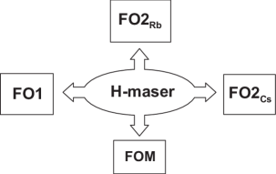
Figure 1: BNM-SYRTE clock ensemble. A single 100 MHz signal from a H-maser is used for frequency comparisons and is distributed to each of the microwave synthesizers of the ¹³³Cs (FO1, FOM, FO2_Cs) and ⁸⁷Rb fountain clocks. In 2001, the Rb fountain has been upgraded and is now a dual fountain using alternately rubidium (FO2_Rb) or cesium atoms (FO2_Cs).

The three fountains have different geometries and operating conditions: the number of detected atoms ranges from $3\times 10^{5}$ to $2\times 10^{6}$ at a temperature of $\sim 1\,\mu$K, the fountain cycle duration from 1.1 to 1.6 s. The Ramsey resonance width is between 0.9 and $1.2$ Hz. In measurements reported here the fractional frequency instability is $(1-2)\times 10^{-13}\tau^{-1/2}$, where $\tau$ is the averaging time in seconds. Fountain comparisons have a typical resolution of $\sim 10^{-15}$ for a 12 hour integration, and each of the four data campaigns lasts from 1 to 2 months during which an accuracy evaluation of each fountain is performed.

Figure 2: The 2002 frequency comparison data. a) H-maser fractional frequency offset versus FOM (black squares), and alternately versus FO2_Rb (open circles) and FO2_Cs (open triangles between dotted lines). b) Fractional frequency differences. Between dotted lines, Cs-Cs comparisons, outside Rb-Cs comparisons. Error bars are purely statistical. They correspond to the Allan standard deviation of the comparisons and do not include contributions from fluctuations of systematic shifts of Table 1.

The 2002 measurements are presented in Fig.2, which displays the maser fractional frequency offset, measured by the Cs fountains FOM and FO2_Cs. Also shown is the H-maser frequency offset measured by the Rb fountain FO2_Rb where the Rb hyperfine frequency is conventionally chosen to be $\nu_{\mathrm{Rb}}(1999)=6\,834\,682\,610.904\,333\,$Hz, our 1999 value. The data are corrected for the systematic frequency shifts listed in Table 1. The H-maser frequency exhibits fractional fluctuations on the order of $10^{-14}$ over a few days, ten times larger than the typical statistical uncertainty resulting from the instability of the fountain clocks. In order to reject the H-maser frequency fluctuations, the fountain data are recorded simultaneously (within a few minutes). The fractional frequency differences plotted in Fig.2 b illustrate the efficiency of this rejection. FO2 is operated alternately with Rb and Cs, allowing both Rb-Cs comparisons and Cs-Cs comparisons (central part of Fig.2) to be performed.

Table 1: Accuracy budget of the fountains involved in the 2002 measurements (FO2 et FOM).

Fountain	FO2Cs	FO2Rb	FOM
Effect	Value & Uncertainty (10${}^{-16})$
2nd order Zeeman	$1773.0\pm 5.2$	$3207.0\pm 4.7$	$385.0\pm 2.9$
Blackbody Radiation	$-173.0\pm 2.3$	$-127.0\pm 2.1$	$-186.0\pm 2.5$
Cold collisions + cavity pulling	$-95.0\pm 4.6$	$0.0\pm 1.0$	$-24.0\pm 4.8$
others	$0.0\pm 3.0$	$0.0\pm 3.0$	$0.0\pm 3.7$
Total uncertainty	8	6	8

Systematic effects shifting the frequency of the fountain standards are listed in Table 1. The quantization magnetic field in the interrogation region is determined with a $0.1$ nT uncertainty by measuring the frequency of a linear field-dependent “Zeeman” transition. The temperature in the interrogation region is monitored with 5 platinum resistors and the uncertainty on the black-body radiation frequency shift corresponds to temperature fluctuations of about 1 K Simon98 . Clock frequencies are corrected for the cold collision and cavity pulling frequency shifts using several methods Pereira02 ; Sortais00 . For Rb, unlike Sortais00 , an optical molasses with a small number of atoms ($\sim 5.4\times 10^{6}$) is used. We thus estimate that these two shifts are smaller than $5\times 10^{-17}$. All other effects do not contribute significantly and their uncertainties are added quadratically. We searched for the influence of synchronous perturbations by changing the timing sequence and the atom launch height. To search for possible microwave leakage, we changed the power ($\times 9$) in the interrogation microwave cavity. No shift was found at a resolution of $10^{-15}$. The shift due to residual coherences and populations in neighboring Zeeman states is estimated to be less than $10^{-16}$. As shown in Wolf01 , the shift due to the microwave photon recoil is very similar for Cs and Rb and smaller than $+1.4\times 10^{-16}$. Relativistic corrections (gravitational redshift and second order Doppler effect) contribute to less than $10^{-16}$ in the clock comparisons.

For the Cs-Cs 2002 comparison, we find:

$$\frac{{\nu_{\mathrm{Cs}}^{\mathrm{FO2}}(2002)}-\nu_{\mathrm{Cs}}^{\mathrm{FOM}}(2002)}{\nu_{\mathrm{Cs}}}=+12(6)(12)\times 10^{-16}$$ (15)

where the first parenthesis reflects the $1\sigma$ statistical uncertainty, and the second the systematic uncertainty, obtained by adding quadratically the inaccuracies of the two Cs clocks (see Table 1). The two Cs fountains are in good agreement despite their significantly different operating conditions (see Table 1), showing that systematic effects are well understood at the $10^{-15}$ level.

In 2002, the ⁸⁷Rb frequency measured with respect to the average ¹³³Cs frequency is found to be:

$$\nu_{\mathrm{Rb}}(2002)=6\,834\,682\,610.904\,324(4)(7)\,\mathrm{Hz}$$ (16)

where the error bars now include FO2_Rb, FO2_Cs and FOM uncertainties. This is the most accurate frequency measurement to date.

Figure 3: Measured ⁸⁷Rb frequencies referenced to the ¹³³Cs fountains over 57 months. The 1999 measurement value ($\nu_{\mathrm{Rb}}(1999)=6\,834\,682\,610.904\,333\,$Hz) is conventionally used as reference. A weighted linear fit to the data gives $\frac{d}{dt}\ln\left(\frac{\nu_{\mathrm{Rb}}}{\nu_{\mathrm{Cs}}}\right)=(0.2\pm 7.0)\times 10^{-16}\,\mathrm{yr}^{-1}$. Dotted lines correspond to the $1\sigma$ slope uncertainty.

In Fig.3 are plotted all our Rb-Cs frequency comparisons. Except for the less precise 1998 data Bize99 , two Cs fountains were used together to perform the Rb measurements. The uncertainties for the 1999 and 2000 measurements were $2.7\times 10^{-15}$, because of lower clock accuracy and lack of rigorous simultaneity in the earlier frequency comparisons Bize01 . A weighted linear fit to the data in Fig.3 determines how our measurements constrain a possible time variation of $\nu_{\mathrm{Rb}}/\nu_{\mathrm{Cs}}$. We find:

$$\frac{d}{dt}\ln\left(\frac{\nu_{\mathrm{Rb}}}{\nu_{\mathrm{Cs}}}\right)=(0.2\pm 7.0)\times 10^{-16}\,\mathrm{yr}^{-1}$$ (17)

which represents a 5-fold improvement over our previous results Bize01 and a 100-fold improvement over the Hg⁺-H hyperfine energy comparison Prestage95 . Using equation 6 and the sensitivity to $\alpha$ in equation 9 and 10, we find that this results implies the following constraint:

$$\frac{d}{dt}\ln\left(\frac{g_{\mathrm{Cs}}}{g_{\mathrm{Rb}}}\alpha^{0.49}\right)=(0.2\pm 7.0)\times 10^{-16}\,\mathrm{yr}^{-1}.$$ (18)

Using the link between g-factors, $m_{q}$ and $\Lambda_{\mathrm{QCD}}$ (ref. Flambaum2003 , eq. 9 and 10), we get:

$$\frac{d}{dt}\ln\left(\alpha^{0.49}\left[m_{q}/\Lambda_{\mathrm{QCD}}\right]^{0.17}\right)=(0.2\pm 7.0)\times 10^{-16}\,\mathrm{yr}^{-1}.$$ (19)

A comparison between the single mercury ¹⁹⁹Hg⁺ ion optical clock and the ¹³³Cs hyperfine splitting has been recently reported by the NIST group Bize03 which (according to eq. 10 and 14) constrains the stability of $\alpha^{6.0}[m_{e}/\Lambda_{\mathrm{QCD}}][m_{q}/\Lambda_{\mathrm{QCD}}]^{0.1}$ at the level of $7\times 10^{-15}$ yr^-1.

III Tests of Local Lorentz Invariance

Local Lorentz Invariance is one of the constituent elements of the Einstein Equivalence Principle (see Sect. 1) and therefore one of the cornerstones of modern physics. It is the fundamental hypothesis of special relativity and is related to the ”constancy of the speed of light”. The central importance of this postulate in modern physics has motivated tremendous work to experimentally test LLI Will ; KostoB . Additionally, nearly all unification theories (in particular string theory) violate the EEP at some level Damour1 which further motivates experimental searches for such violations of the universality of free fall Damour94 and of Lorentz invariance Kosto1 ; Kosto2 .

We report here on experimental tests of LLI using a cryogenic sapphire oscillator and a hydrogen maser. The relative frequency of the two clocks is monitored looking for a Lorentz violating signal which would modulate that frequency at, typically, sidereal and semi-sidereal periods due to the movement of the lab with the rotation of the Earth. We set limits on parameters that describe such Lorentz violating effects, improving our previous results Wolf by a factor 2 and the best other results Schiller ; Muller by up to a factor 70.

Many modern experiments that test LLI rely essentially on the stability of atomic clocks and macroscopic resonators Brillet ; KT ; Hils ; Schiller ; Wolf ; Lipa ; Muller , therefore improvements in oscillator technology have gone hand in hand with improved tests of LLI. Our experiment is no exception, the large improvements being a direct result of the excellent stability of our cryogenic sapphire oscillator. Additionally its operation at a microwave frequency allows a direct comparison to a hydrogen maser which provides a highly stable and reliable reference frequency.

Numerous test theories that allow the modeling and interpretation of experiments that test LLI have been developed. Kinematical frameworks Robertson ; MaS postulate a simple parametrisation of the Lorentz transformations with experiments setting limits on the deviation of those parameters from their special relativistic values. A more fundamental approach is offered by theories that parametrise the coupling between gravitational and non-gravitational fields (TH$\epsilon\mu$ LightLee ; Will ; Blanchet or $\chi$g Ni formalisms) which allow the comparison of experiments that test different aspects of the EEP. Finally, formalisms based on string theory KostoB ; Damour1 ; Damour94 ; Kosto1 have the advantage of being well motivated by theories of physics that are at present the only candidates for a unification of gravity and the other fundamental forces of nature.

III.1 Theory

Owing to their simplicity the kinematical frameworks of Robertson ; MaS have been widely used to model and interpret many previous experiments testing LLI Brillet ; Hils ; Schiller ; Wolf ; Riis ; WP and we will follow that route. An analysis based on the more fundamental ”Standard Model Extension” (SME) Kosto1 ; KM is under way and will be published shortly.

By construction kinematical frameworks do not allow for any dynamical effects on the measurement apparatus. This implies that in all inertial frames two clocks of different nature (e.g. based on different atomic species) run at the same relative rate and two length standards made of different materials keep their relative lengths. Coordinates are defined by the clocks and length standards, and only the transformations between those coordinate systems are modified. In general this leads to observable effects on light propagation in moving frames but, by definition, to no observable effects on clocks and length standards. In particular, no attempt is made at explaining the underlying physics (e.g. modified Maxwell and/or Dirac equations) that could lead to Lorentz violating light propagation but leave e.g. atomic energy levels unchanged. On the other hand dynamical frameworks (e.g. the TH$\epsilon\mu$ formalism or the SME) in general use a modified general Lagrangian that leads to modified Maxwell and Dirac equations and hence to Lorentz violating light propagation and atomic properties, which is why they are considered more fundamental and more complete than the kinematical frameworks. Furthermore, as shown in KM , the SME is kept sufficiently general to, in fact, encompass the kinematical frameworks and some other dynamical frameworks (in particular the TH$\epsilon\mu$ formalism) as special cases, although there are no simple and direct relationships between the respective parameters.

Concerning our experiment the SME allows the calculation of Lorentz violating effects on the fields inside the sapphire resonator, on the properties of the sapphire crystal itself and on the hydrogen maser transition. As shown in Muller2 the effect on the sapphire crystal amounts to only a few percent of the direct effect on the fields, and KL show that the hydrogen $m_{F}=0\to m^{\prime}_{F}=0$ clock transition is not affected to first order. Hence the total effect is dominated by the Lorentz violating properties of the electromagnetic fields inside the resonator which can be calculated following the principles laid down in KM . An analysis of our experiment in that framework is currently being carried out, and the results will be published elsewhere in the near future. In this paper we concentrate on the analysis using the kinematical framework of Mansouri and Sexl MaS .

The Robertson, Mansouri & Sexl Framework

Kinematical frameworks for the description of Lorentz violation have been pioneered by Robertson Robertson and further refined by Mansouri and Sexl MaS and others. Fundamentally the different versions of these frameworks are equivalent, and relations between their parameters are readily obtained. As mentioned above these frameworks postulate generalized transformations between a preferred frame candidate $\Sigma(T,{\bf X})$ and a moving frame ${\rm S}(t,{\bf x})$ where it is assumed that in both frames coordinates are realized by identical standards. We start from the transformations of MaS (in differential form) for the case where the velocity of $S$ as measured in $\Sigma$ is along the positive X-axis, and assuming Einstein synchronization in $S$ (we will be concerned with signal travel times around closed loops so the choice of synchronization convention can play no role):

$$dT={1\over a}\left(dt+{vdx\over c^{2}}\right);dX={dx\over b}+{v\over a}\left(dt+{vdx\over c^{2}}\right);dY={dy\over d};dZ={dz\over d}$$ (20)

with $c$ the velocity of light in vacuum in $\Sigma$. Using the usual expansion of the three parameters $(a\approx 1+\alpha_{\mathrm{MS}}{v^{2}/c^{2}}+{\cal O}(4);b\approx 1+\beta_{\mathrm{MS}}{v^{2}/c^{2}}+{\cal O}(4);d\approx 1+\delta_{\mathrm{MS}}{v^{2}/c^{2}}+{\cal O}(4))$, setting $c^{2}dT^{2}=dX^{2}+dY^{2}+dZ^{2}$ in $\Sigma$, and transforming according to (20) we find the coordinate travel time of a light signal in S:

$$dt={dl\over c}\left(1-\left(\beta_{\mathrm{MS}}-\alpha_{\mathrm{MS}}-1\right){v^{2}\over c^{2}}-\left({1\over 2}-\beta_{\mathrm{MS}}+\delta_{\mathrm{MS}}\right){\rm sin}^{2}\theta{v^{2}\over c^{2}}\right)+{\cal O}(4)$$ (21)

where $dl=\sqrt{dx^{2}+dy^{2}+dz^{2}}$ and $\theta$ is the angle between the direction of light propagation and the velocity v of S in $\Sigma$. In special relativity $\alpha_{\mathrm{MS}}=-1/2;\beta_{\mathrm{MS}}=1/2;\delta_{\mathrm{MS}}=0$ and (20) reduces to the usual Lorentz transformations. Generally, the best candidate for $\Sigma$ is taken to be the frame of the cosmic microwave background (CMB) Fixsen ; Lubin with the velocity of the solar system in that frame taken as $v_{\odot}\approx 377$ km/s, decl. $\approx-6.4^{\circ}$, $RA\approx 11.2$h.

Michelson-Morley type experiments MM ; Brillet determine the coefficient $P_{MM}=(1/2-\beta_{\mathrm{MS}}+\delta_{\mathrm{MS}})$ of the direction dependent term. For many years the most stringent limit on that parameter was $|P_{MM}|\leq 5\times 10^{-9}$ determined over 23 years ago in an outstanding experiment Brillet . Our experiment confirms that result with roughly equivalent uncertainty $(2.2\times 10^{-9})$. Recently an improvement to $|P_{MM}|\leq 1.5\times 10^{-9}$ has been reported Muller . Kennedy-Thorndike experiments KT ; Hils ; Schiller measure the coefficient $P_{KT}=(\beta_{\mathrm{MS}}-\alpha_{\mathrm{MS}}-1)$ of the velocity dependent term. The most stringent limit Schiller on $|P_{KT}|$ has been recently improved from Hils by a factor 3 to $|P_{KT}|\leq 2.1\times 10^{-5}$. We improve this result by a factor of 70 to $|P_{KT}|\leq 3.0\times 10^{-7}$. Finally clock comparison and Doppler experiments Riis ; Grieser ; WP measure $\alpha_{\mathrm{MS}}$, currently limiting it to $|\alpha_{\mathrm{MS}}+1/2|\leq 8\times 10^{-7}$. The three types of experiments taken together then completely characterize any deviation from Lorentz invariance in this particular test theory, with present limits summarized in Table 2.

Table 2: Present limits on Lorentz violating parameters in the framework of MaS

Reference	$\alpha_{\mathrm{MS}}+1/2$	$1/2-\beta_{\mathrm{MS}}+\delta_{\mathrm{MS}}$	$\beta_{\mathrm{MS}}-\alpha_{\mathrm{MS}}-1$
Riis ; Grieser ; WP	$\leq 8\times 10^{-7}$	-	-
Brillet	-	$\leq 5\times 10^{-9}$	-
Muller	-	$(2.2\pm 1.5)\times 10^{-9}$	-
Schiller	-	-	$(1.9\pm 2.1)\times 10^{-5}$
our previous results Wolf	-	$(1.5\pm 4.2)\times 10^{-9}$	$(-3.1\pm 6.9)\times 10^{-7}$
this work	-	$(1.2\pm 2.2)\times 10^{-9}$	$(1.6\pm 3.0)\times 10^{-7}$

Our cryogenic oscillator consists of a sapphire crystal of cylindrical shape operating in a whispering gallery mode (see Fig. 4 for a schematic drawing and Chang ; Mann for a detailed description). Its coordinate frequency can be expressed by $\nu=m/t_{c}$ where $t_{c}$ is the coordinate travel time of a light signal around the circumference of the cylinder (of radius $r$) and $m$ is a constant. From (21) the relative frequency difference between the sapphire oscillator and the hydrogen maser (which, by definition, realizes coordinate time in S masercom ) is

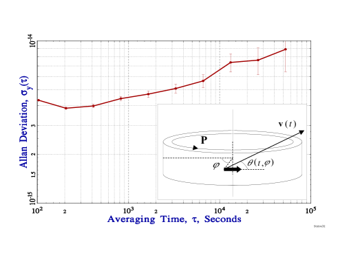
Figure 4: Typical relative frequency stability of the CSO - H-maser difference after removal of a linear frequency drift. The inset is a schematic drawing of the cylindrical sapphire oscillator with the Poynting vector $\bf P$ in the whispering gallery (WG) mode, the velocity ${\bf v}(t)$ of the cylinder with respect to the CMB, and the relevant angles for a photon in the WG mode.

$${\Delta\nu(t)\over\nu_{0}}=P_{KT}{v(t)^{2}\over c^{2}}+P_{MM}{v(t)^{2}\over c^{2}}{1\over 2\pi}\int_{0}^{2\pi}{\rm sin}^{2}\theta(t,\varphi)d\varphi+{\cal O}(3)$$ (22)

where $\nu_{0}=m/(2\pi r/c)$, $v(t)$ is the (time dependent) speed of the lab in $\Sigma$, and $\varphi$ is the azimuthal angle of the light signal in the plane of the cylinder. The periodic time dependence of $v$ and $\theta$ due to the rotation and orbital motion of the Earth with respect to the CMB frame allow us to set limits on the two parameters in (22) by adjusting the periodic terms of appropriate frequency and phase (see Mike for calculations of similar effects for several types of oscillator modes). Given the limited durations of our data sets ($\leq$ 15 days) the dominant periodic terms arise from the Earth’s rotation, so retaining only those we have ${\bf v}(t)={\bf u}+{\bf\Omega}\times{\bf R}$ with ${\bf u}$ the velocity of the solar system with respect to the CMB, ${\bf\Omega}$ the angular velocity of the Earth, and ${\bf R}$ the geocentric position of the lab. We then find after some calculation.

$$\begin{array}[]{cl}\Delta\nu/\nu_{0}&=P_{KT}(H{\rm sin}\lambda)\\ &+P_{MM}(A{\rm cos}\lambda+B{\rm cos}(2\lambda)+C{\rm sin}\lambda+D{\rm sin}\lambda{\rm cos}\lambda+E{\rm sin}\lambda{\rm cos}(2\lambda))\end{array}$$ (23)

where $\lambda=\Omega t+\phi$, and A-E and $\phi$ are constants depending on the latitude and longitude of the lab $(\approx 48.7^{\circ}$N and $2.33^{\circ}$E for Paris). Numerically $H\approx-2.6\times 10^{-9}$, $A\approx-8.8\times 10^{-8}$, $B\approx 1.8\times 10^{-7}$, C-E of order $10^{-9}$. We note that in (23) the dominant time variations of the two combinations of parameters are in quadrature and at twice the frequency which indicates that they should decorelate well in the data analysis allowing a simultaneous determination of the two (as confirmed by the correlation coefficients given in Sect. 3.2). Adjusting this simplified model to our data we obtain results that differ by less than 10% from the results presented in Sect. 3.2 that were obtained using the complete model ((22) including the orbital motion of the Earth).

III.2 Experimental Results

The cryogenic sapphire oscillator (CSO) is compared to a commercial (Datum Inc.) active hydrogen maser whose frequency is also regularly compared to caesium and rubidium atomic fountain clocks in the laboratory Bize01 . The CSO resonant frequency at 11.932 GHz is compared to the 100 MHz output of the hydrogen maser. The maser signal is multiplied up to 12 GHz of which the CSO signal is subtracted. The remaining $\approx$ 67 MHz signal is mixed to a synthesizer signal at the same frequency and the low frequency beat at $\approx$ 64 Hz is counted, giving access to the frequency difference between the maser and the CSO. The instability of the comparison chain has been measured and does not exceed a few parts in $10^{16}$. The typical stability of the measured CSO - maser frequency after removal of a linear frequency drift is shown in Fig. 4. Since September 2002 we are taking continuous temperature measurements on top of the CSO dewar and behind the electronics rack. Starting January 2003 we have implemented an active temperature control of the CSO room and changed some of the electronics. As a result the diurnal and semi-diurnal temperature variations during measurement runs ($\approx$ 2 weeks) were greatly reduced to less than $0.025^{\circ}$ C in amplitude (best case), and longer and more reliable data sets became available.

Our previously published results Wolf are based on data sets taken between Nov. 2001 and Sep. 2002 which did not all include regular temperature monitoring and control. Here we use only data that was permanently temperature controlled, 13 data sets in total spanning Sept. 2002 to Aug. 2003, of differing lengths (5 to 16 days, 140 days in total). The sampling time for all data sets was $100$ s except two data sets with $\tau_{0}=12$ s. To make the data more manageable we first average all points to $\tau_{0}=2500$ s. For the data analysis we simultaneously adjust an offset and a rate (natural frequency drift, typically $\approx 1.7\times 10^{-18}$ s^-1) per data set and the two parameters of the model (22). In the model (22) we take into account the rotation of the Earth and the Earth’s orbital motion, the latter contributing little as any constant or linear terms over the durations of the individual data sets are absorbed by the adjusted offsets and rates.

When carrying out an ordinary least squares (OLS) adjustment we note that the residuals have a significantly non-white behavior as one would expect from the slope of the Allan deviation of Fig. 4. The power spectral density (PSD) of the residuals when fitted with a power law model of the form $S_{y}(f)=kf^{\mu}$ yields typically $\mu\approx-1.5$ to $-2$. In the presence of non-white noise OLS is not the optimal regression method lss ; Draper as it can lead to significant underestimation of the parameter uncertainties lss .

An alternative method is weighted least squares (WLS) Draper which allows one to account for non-white noise processes in the original data by pre-multiplying both sides of the design equation (our equation (22) plus the offsets and rates) by a weighting matrix containing off diagonal elements. To determine these off diagonal terms we first carry out OLS and adjust the $S_{y}(f)=kf^{\mu}$ power law model to the PSD of the post-fit residuals determining a value of $\mu$ for each data set. We then use these $\mu$ values to construct a weighting matrix following the method of fractional differencing described, for example, in lss . Figure 5 shows the resulting values of the two parameters ($P_{KT}$ and $P_{MM}$) for each individual data set. A global WLS fit of the two parameters and the 13 offsets and drifts yields $P_{MM}=(1.2\pm 1.9)\times 10^{-9}$ and $P_{KT}=(1.6\pm 2.3)\times 10^{-7}$ ($1\sigma$ uncertainties), with the correlation coefficient between the two parameters less than 0.01 and all other correlation coefficients $<0.06$. The distribution of the 13 individual values around the ones obtained from the global fit is well compatible with a normal distribution ($\chi^{2}$ = 10.7 and 14.6 for $P_{MM}$ and $P_{KT}$ respectively).

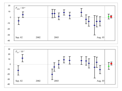
Figure 5: Values of the two parameters ($P_{KT}$ and $P_{MM}$) from a fit to each individual data set (blue diamonds) and a global fit to all the data (red squares). For comparison our previously published results Wolf are also shown (green triangles). The error bars indicate the combined uncertainties from statistics and systematic effects.

Systematic effects at diurnal or semi-diurnal frequencies with the appropriate phase could mask a putative sidereal signal. The statistical uncertainties of $P_{MM}$ and $P_{KT}$ obtained from the WLS fit above correspond to sidereal and semi-sidereal terms (from (23)) of $\approx 7\times 10^{-16}$ and $\approx 4\times 10^{-16}$ respectively so any systematic effects exceeding these limits need to be taken into account in the final uncertainty. We expect the main contributions to such effects to arise from temperature, pressure and magnetic field variations that would affect the hydrogen maser, the CSO and the associated electronics, and from tilt variations of the CSO which are known to affect its frequency. Measurements of the tilt variations of the CSO show amplitudes of 4.6 $\mu$rad and 1.6 $\mu$rad at diurnal and semi-diurnal frequencies.

To estimate the tilt sensitivity we have intentionally tilted the oscillator by $\approx$ 5 mrad off its average position which led to relative frequency variations of $\approx 3\times 10^{-13}$ from which we deduce a tilt sensitivity of $\approx 6\times 10^{-17}\mu$rad^-1. This value corresponds to a worst case scenario as we expect a quadratic rather than linear frequency variation for small tilts around the vertical. Even with this pessimistic estimate diurnal and semi-diurnal frequency variations due to tilt do not exceed $3\times 10^{-16}$ and $1\times 10^{-16}$ respectively and are therefore negligible with respect to the statistical uncertainties.

In December 2002 we implemented an active temperature stabilization inside an isolated volume ($\approx 15{\rm m}^{3}$) that included the CSO and all the associated electronics. The temperature was measured continously in two fixed locations (behind the electronics rack and on top of the dewar). For the best data sets the measured temperature variations did not exceed 0.02/0.01 ^∘C in amplitude for the diurnal and semi-diurnal components. In the worst cases (the two 2002 data sets and some data sets taken during a partial air conditioning failure) the measured temperature variations could reach 0.26/0.08 ^∘C. When intentionally heating and cooling the CSO lab by $\approx 3^{\circ}$C we see frequency variations of $\approx 5\times 10^{-15}$ per ^∘C. This is also confirmed when we induce a large sinusoidal temperature variation ($\approx 1.5^{\circ}$C amplitude). Using this we can calculate a value for temperature induced frequency variations at diurnal and semi-diurnal frequencies for each data set, obtaining values that range from $\approx 1.3\times 10^{-15}$ to $\approx 5\times 10^{-17}$.

The hydrogen maser is kept in a dedicated, environmentally controlled clock room. Measurements of magnetic field, temperature and atmospheric pressure in that room and the maser sensitivities as specified by the manufacturer allow us to exclude any systematic effects on the maser frequency that would exceed the statistical uncertainties above and the systematic uncertainties from temperature variations in the CSO lab.

Our final uncertainties (the error bars in Fig. 5) are the quadratic sums of the statistical uncertainties from the WLS adjustment for each data set and the systematic uncertainties calculated for each data set from (23) and the measured temperature variations. For the global adjustment we average the systematic uncertainties from the individual data sets obtaining $\pm 1.2\times 10^{-9}$ on $P_{MM}$ and $\pm 1.9\times 10^{-7}$ on $P_{KT}$. Adding these quadratically to the WLS statistical uncertainties of the global adjustment we obtain as our final result $P_{MM}=(1.2\pm 2.2)\times 10^{-9}$ and $P_{KT}=(1.6\pm 3.0)\times 10^{-7}$ ($1\sigma$ uncertainties).

IV Conclusion and Outlook

We have reported on two different tests of the Einstein Equivalence Principle (EEP) using the comparison of atomic clocks with different atomic species on one hand, and the comparison of an atomic clock and a cryogenic sapphire cavity oscillator on the other. The two experiments are interpreted as testing Local Position Invariance (LPI) and Local Lorentz Invariance (LLI) respectively which are both constituent elements of the EEP.

The test of LPI is based on the comparison of the hyperfine transitions in ⁸⁷Rb and ¹³³Cs using atomic fountains that presently reach uncertainties of $(6-8)\times 10^{-16}$. Such measurements were repeated over the last 5 years to search for a time variation that would indicate a violation of LPI. Our present results limit a linear variation to $\frac{d}{dt}\ln\left(\frac{\nu_{\mathrm{Rb}}}{\nu_{\mathrm{Cs}}}\right)=(0.2\pm 7.0)\times 10^{-16}\,\mathrm{yr}^{-1}$ which represents a 5-fold improvement over our previous results Bize01 and a 100-fold improvement over the Hg⁺-H hyperfine energy comparison Prestage95 . When interpreting the results as a limit on the time variation of fundamental constants (c.f. Sect. 2.1) we obtain

$$\left|0.49\frac{\dot{\alpha}}{\alpha}+0.17\frac{\dot{m_{q\Lambda}}}{m_{q\Lambda}}\right|\leq 7\times 10^{-16}\,\mathrm{yr}^{-1}$$ (24)

where $m_{q\Lambda}$ stands for $m_{q}/\Lambda_{\mathrm{QCD}}$. By itself this experiment limits the time variation of a combination of two of the three fundamental constants of Sect. 2.1. The ¹⁹⁹Hg⁺ to ¹³³Cs comparisons by the NIST group Bize03 provide

$$\left|6.0\frac{\dot{\alpha}}{\alpha}+0.1\frac{\dot{m_{q\Lambda}}}{m_{q\Lambda}}+\frac{\dot{m_{e\Lambda}}}{m_{e\Lambda}}\right|\leq 7\times 10^{-15}\,\mathrm{yr}^{-1}$$ (25)

where $m_{e\Lambda}$ stands for $m_{e}/\Lambda_{\mathrm{QCD}}$. Combining these two results we have two constraints on the variation of the three fundamental constants, with the missing third constraint requiring the comparison over time with a fourth atomic transition (c.f. Sect. 2.1).

The test of LLI is based on the comparison of a hydrogen maser clock to a cryogenic sapphire microwave cavity. This experiment simultaneously constrains two combinations of the three parameters of the Mansouri and Sexl test theory (previously measured individually by Michelson-Morley and Kennedy-Thorndike experiments). We obtain $\delta_{\mathrm{MS}}-\beta_{\mathrm{MS}}+1/2=1.2(1.9)(1.2)\times 10^{-9}$ which is of the same order as the best previous results Brillet ; Muller , and $\beta_{\mathrm{MS}}-\alpha_{\mathrm{MS}}-1=1.6(2.3)(1.9)\times 10^{-7}$ which improves the best previous limit Schiller by a factor of 70 (the first bracket indicates the $1\sigma$ uncertainty from statistics the second from systematic effects). We improve our own previous results Wolf by about a factor 2 due to more and longer data sets and to improved temperature control of the experiment. We note that our value on $\delta_{\mathrm{MS}}-\beta_{\mathrm{MS}}+1/2$ is compatible with the slightly significant recent result of Muller who obtained $\delta_{\mathrm{MS}}-\beta_{\mathrm{MS}}+1/2=(2.2\pm 1.5)\times 10^{-9}$.

As a result of our experiment the Lorentz transformations are confirmed in this particular test theory with an overall uncertainty of $\leq 8\times 10^{-7}$ limited now by the determination of $\alpha_{\mathrm{MS}}$ from Doppler and clock comparison experiments Riis ; WP . This is likely to be improved in the coming years by experiments such as ACES (Atomic Clock Ensemble in Space ACES ) that will compare ground clocks to clocks on the international space station aiming at a 10 fold improvement on the determination of $\alpha_{\mathrm{MS}}$.

In the future, the two tests of LPI and LLI presented here are expected to further improve due to improvements in the accuracies of the atomic clocks involved and due to new experimental strategies, ultimately leading to space-borne versions of the experiments.

Ongoing efforts are expected to improve the accuracy of both ⁸⁷Rb and ¹³³Cs to the $10^{-16}$ level. The corresponding limit to variations of fundamental constants will then be decreased to $\sim 10^{-16}$ yr^-1 or less. Recent advances in the field of optical frequency metrology will probably lead optical frequency standards to surpass microwave clocks. Comparing such standards to each other will provide very stringent limits to the variation of the fine structure constant $\alpha$. To keep the constraints to the variation of $m_{q}/\Lambda_{\mathrm{QCD}}$ and $m_{e}/\Lambda_{\mathrm{QCD}}$ at the same level, further efforts and new methods will have to be invented to improve microwave clocks. These tests will also greatly benefit from a new generation of time/frequency transfer at the $10^{-16}$ level which is currently under development for the ESA space mission ACES which will fly ultra-stable clocks on board the international space station in 2006 ACES and a similar project conducted by NASA. These missions will allow highly precise comparisons between clocks developed in distant laboratories and based on different atomic species and/or different technologies.

Concerning the test of LLI, new proposals have been made to use two orthogonal resonators or two orthogonal modes in the same sapphire resonator placed on a rotating platform Mike . Such a set-up is likely to improve the tests of LLI by several orders of magnitude as the relevant time variations will now be at the rotation frequency ($\approx 0.01-0.1$ Hz) which is the range in which such resonators are the most stable ($\approx$ 100 fold better stability). Additionally many systematic effects are likely to cancel between the two orthogonal oscillators or modes and the remaining ones are likely to be less coupled to the rotation frequency than to the sidereal frequencies used in our experiment. Ultimately, it has been proposed Lammerzahl2001 to conduct these tests on board an Earth orbiting satellite, again with a potential gain of several orders of magnitudes over current limits.

References

- (1) Will C.M., Theory and Experiment in Gravitational Physics, revised edition, Cambridge U. Press, (1993).
- (2) W.J. Marciano, Phys.Rev. Lett. 52, 489 (1984).
- (3) T. Damour and A. Polyakov, Nucl. Phys. B 423, 532 (1994).
- (4) T. Damour, F. Piazza, and G. Veneziano, Phys. Rev. Lett. 89, 081601 (2002).
- (5) J.K. Webb et al., Phys. Rev. Lett. 87, 091301 (2001).
- (6) H. Marion et al., Phys. Rev. Lett 90, 150801 (2003).
- (7) J.D. Prestage, R.L. Tjoelker and L. Maleki, Phys. Rev. Lett. 74, 3511 (1995).
- (8) D.J. Berkeland et al., Phys. Rev. Lett. 80, 2089 (1998).
- (9) M. Niering et al., Phys. Rev. Lett. 84, 5496 (2000).
- (10) J. Helmcke et al, IEEE Trans. Instrum. Meas. 52, 250 (2003).
- (11) S. Bize et al., Phys. Rev. Lett 90, 150802 (2003).
- (12) J. Stenger et al., Opt. Lett. 26, 1589 (2001).
- (13) E. Peik et al., in Proc. of the Joint Mtg. IEEE Intl. Freq. Cont. Symp. and EFTF Conf., (2003).
- (14) V.V. Flambaum, ArXiv:physics/0302015 (2003).
- (15) V.A. Dzuba, V.V. Flambaum and J.K. Webb, Phys. Rev. A 59, 230 (1999).
- (16) V.A. Dzuba, V.V. Flambaum and J.K. Webb, Phys. Rev. Lett. 82, 888 (1999).
- (17) V.A. Dzuba, V.V. Flambaum and J.K. Webb, Phys. Rev. A 61, 034502 (2000).
- (18) S.G. Karshenboïm, Can. J. Phys. 47, 639 (2000).
- (19) V.A. Dzuba, V.V. Flambaum and M.V. Marchenko, ArXiv:physics/0305066 (2003).
- (20) I. Courtillot et al, Phys. Rev. A 68, 030501 (2003).
- (21) H. Katori et al, ArXiv:physics/0309043 (2003).
- (22) M. Takamoto and H. Katori, ArXiv:physics/0309004 (2003).
- (23) D.J. Wineland et al., in Proc. of the Joint Mtg. IEEE Intl. Freq. Cont. Symp. and EFTF Conf., p 68. (2003).
- (24) A. Clairon et al., in Proc. of the 5th Symposium on Frequency Standards and Metrology, ed. J. Bergquist (World Scientific, Singapore, 1995), p. 49.
- (25) S. Bize et al., in Proc. of the 6th Symposium on Frequency Standards and Metrology (World Scientific, Singapore, 2001), p 53.
- (26) S. Bize et al., Europhys. Lett. 45, 558 (1999).
- (27) E. Simon et al., Phys. Rev. A 57, 436 (1998).
- (28) F. Pereira Dos Santos et al., Phys. Rev. Lett. 89, 233004 (2002).
- (29) Y. Sortais et al., Phys. Rev. Lett. 85, 3117 (2000).
- (30) P. Wolf et al., in Proc. of the 6th Symposium on Frequency Standards and Metrology (World Scientific, Singapore, 2001), p 593.
- (31) Kostelecky V.A. ed., CPT and Lorentz Symmetry II, World Scientific, Singapore, (2002).
- (32) Damour T., gr-qc/9711060 (1997).
- (33) Colloday D. and Kostelecky V.A., Phys. Rev. D55, 6760, (1997).
- (34) Bluhm R. et al., Phys. Rev. Lett. 88, 9, 090801, (2002).
- (35) Brillet A. and Hall J.L., Phys. Rev. Lett. 42, 9, 549, (1979).
- (36) Kennedy R.J. and Thorndike E.M., Phys. Rev. B42, 400, (1932).
- (37) Hils D. and Hall J.L., Phys. Rev. Lett., 64, 15, 1697, (1990).
- (38) Braxmaier C. et al., Phys. Rev. Lett. 88, 1, 010401, (2002).
- (39) Wolf P. et al., Phys. Rev. Lett. 90, 6, 060402, (2003).
- (40) Lipa J.A. et al. Phys. Rev. Lett. 90, 6, 060403, (2003).
- (41) Müller H. et al., Phys. Rev. Lett. 91, 2, 020401, (2003).
- (42) Robertson H.P., Rev. Mod. Phys. 21, 378 (1949).
- (43) Mansouri R. and Sexl R.U., Gen. Rel. Grav. 8, 497, 515, 809, (1977).
- (44) Lightman A.P. and Lee D.L., Phys. Rev. D8, 2, 364, (1973).
- (45) Blanchet L., Phys. Rev. Lett. 69, 4, 559, (1992).
- (46) Ni W.-T., Phys. Rev. Lett. 38, 301, (1977).
- (47) Riis E. et al., Phys. Rev. Lett. 60, 81, (1988).
- (48) Wolf P. and Petit G., Phys. Rev. A56, 6, 4405, (1997).
- (49) Kostelecky A.V. and Mewes M., Phys. Rev. D66, 056005, (2002).
- (50) Fixsen D.J. et al., Phys. Rev. Lett. 50, 620, (1983).
- (51) Lubin et al., Phys. Rev. Lett. 50, 616, (1983).
- (52) Michelson A.A. and Morley E.W., Am. J. Sci., 34, 333, (1887).
- (53) Grieser R. et al., Appl. Phys. B59, 127, (1994).
- (54) Chang S., Mann A.G. and Luiten A.N., Electron. Lett. 36, 5, 480, (2000).
- (55) Mann A.G., Chang S. and Luiten A.N., IEEE Trans. Instrum. Meas. 50, 2, 519, (2001).
- (56) We assume here that local position invariance (c.f. Sect. 2) is sufficiently verified so that the variation of the maser frequency due to the diurnal variation of the local gravitational potential is negligible. Indeed the results of i̧teBauch imply that such variations should not exceed 2 parts in which is significantly below our noise level.
- (57) Bauch A., Weyers S., Phys. Rev. D65, 081101, (2002)
- (58) Tobar M.E. et al., Phys. Lett. A300, 33, (2002).
- (59) Müller H. et al., Phys. Rev. D67, 056006, (2003).
- (60) Kostelecky and Lane, Phys. Rev. D60, 116010, (1999).
- (61) Schmidt L.S., Metrologia 40, in press, (2003).
- (62) Draper N.R. and Smith H., Applied Regression Analysis, Wiley, (1966).
- (63) Salomon C., et al., C.R. Acad. Sci. Paris, 2, 4, 1313, (2001).
- (64) Lämmerzahl C. et al., Class. Quant. Grav., 18, 2499, (2001).