The ISO-LWS far-infrared spectra of pre-Main Sequence objects.

Milena Benedettini, Stefano Pezzuto, Luigi Spinoglio, Paolo Saraceno, Anna Maria Di Giorgio

CNR – Istituto di Fisica dello Spazio Interplanetario, Area di Ricerca di Tor Vergata, via del Fosso del Cavaliere 100, 00133, Roma, Italy

Running title: The ISO-LWS FIR spectra of PMS objects.

To be published in the book “Recent Research Developments in Molecular and Cellular Astronomy & Astrophysics”

ABSTRACT

The Long Wavelength Spectrometer (LWS) on board the Infrared Space Observatory (ISO) satellite has allowed for the first time to investigate the whole far infrared (FIR) part of the spectrum (from 43 to 197 $\mu$m), inaccessible from the ground. The FIR spectrum is crucial for the study of the early phases of protostellar evolution since the peak of the continuum emission of the protostars falls around 100 $\mu$m  and many molecular species emit in this range.

In this paper we review the main results of the spectroscopic observations carried out with the LWS on a sample of pre-Main Sequence objects in different evolutionary stages. The FIR spectra are characterized by a strong continuum with superimposed atomic and molecular emission lines. The fine structure lines emitted by the OI and CII atoms are present in all the objects of our sample while emission from molecular species (CO, H₂O and OH) dominate the spectrum of the younger and more embedded objects; lines of highly ionized atoms (OIII, NIII, NII) are present only in high luminosity sources. We will show how both the FIR continuum and the emission lines are powerful indicators of the evolutionary status of young embedded objects.

The analysis of the LWS spectra has allowed to study only the average properties of the young stellar objects, due to the large field of view ($\sim$ 80 arcsec), the limited sensitivity and the poor spectral resolution ($\sim$ 200) of the instrument in its grating mode. The higher spatial and spectral resolutions of the instruments on board the Herschel satellite will allow to address in deeper detail the scientific problems highlighted by the ISO results.

1 INTRODUCTION

During the early phases of the star formation process the spectral energy distribution (SED) of a protostar has the shape of a cold blackbody (few tens of K) modified by the emissivity of the dust of the molecular cloud where the object is forming. The central object, even when already formed, is not visible at any wavelength since the surrounding dust envelope completely obscures the inner region. As the evolution goes on, the optical depth of the dust decreases making the central object visible in the near infrared until it appears in the optical and its spectrum looks like that of a normal star with an infrared excess due to the residual circumstellar material. At the typical temperatures of pre-Main Sequence (PMS) objects (T=30-80 K) the dust emission peaks in the far infrared (FIR) between 50-200 $\mu$m. The warm circumstellar envelope is predicted to emit a rich FIR spectrum [1] where the prominent features are the water and carbon monoxide rotational lines and the atomic oxygen fine structure lines.

The early stage of the star formation process is also characterized by the presence of energetic mass ejections which interact with the surrounding molecular cloud giving rise to bipolar outflows. The molecular outflow is thought to be the mechanism through which the accreting central object loses the exceeding angular momentum and therefore it plays an important role in stopping the gravitational collapse, thus setting the final mass of the star. Molecular outflows display a large range of excitation conditions, due to the complex way in which the interaction between stellar winds/jets and ambient medium is taking place. Ground based observations of molecular emission lines at mm wavelengths, trace the large scale material at excitation temperatures of about 10-20 K and vibrational lines of molecular Hydrogen at NIR wavelengths probe the highly excited gas (at T${}_{ex}\sim$ 10⁴ K) along the flow axis. However the presence of gas excited at intermediate temperature, i.e. 100-2000 K, can only be traced by FIR space borne observations.

The evolutionary status of the PMS objects cannot be derived by directly observing the stellar radiation, which is only visible during the late phases of star formation, but can be estimated only indirectly by observing the continuum, atomic and molecular emission of the circumstellar envelope or/and of the outflow. Unfortunately, most of the emission falls in the FIR and it is inaccessible from the ground. So far, the methods commonly used to classify the PMS objects have been mainly based on the characterization of the shape of the SED at near and mid infrared wavelengths through the value of the spectral index $\alpha$. Lada & Wilking [2] first classified low-mass protostellar objects considering three different classes defined by the value of $\alpha$ in the range 2–10 $\mu$m  (then extended to 25 $\mu$m  with the IRAS mission). This classification was followed by the work of Adams, Lada & Shu [3] who associated to each class a different evolutionary stage. Successively Andrè, Ward-Thompson & Barsony [4] introduced a new class of objects still younger than the previous classes. The net result of all these works is the classification of low-mass pre-Main Sequence (PMS) sources in four different classes (see Fig. 1), proceeding from the youngest to the oldest they are:

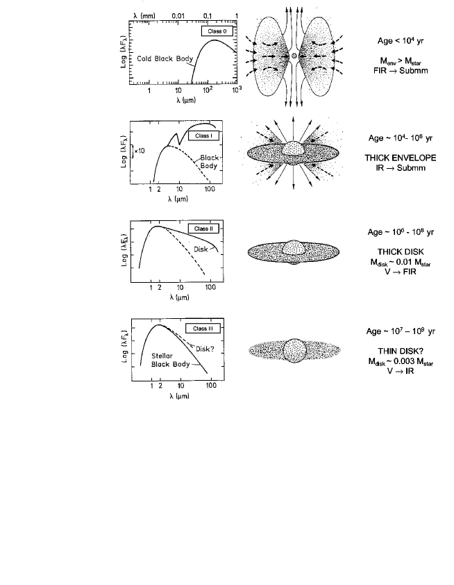
Figure 1: A scheme of the classification of the low-mass PMS objects, adapted from the original figure of [44].

• Class 0: since they are visible only at $\lambda>$ 10 $\mu$m, the spectral index $\alpha$ cannot be derived. They are identified by the ratio between the submillimeter ($\lambda>$350$\mu$m) and the bolometric luminosity L_submm/L${}_{\rm bol}>$5$\times$10^-3. They are newly formed protostars in the main accretion phase, when the mass of the central object is still less than that of the circumstellar material. The central source is completely obscured by the envelope. The spectrum is that of gray body with temperature $\sim$ 25–35 K. Strong and collimated outflows are associated with these objects which have ages $<$10⁴ yr.

• Class I: with $\alpha<$ 0 between 2 and 25 $\mu$m. The spectrum steeply increases in the mid-infrared due to the optically thick envelope. They represent protostars in the final phase of accretion when the stellar winds are dispersing the circumstellar envelope but usually they are not yet visible in the optical. The typical age is between 10⁴ to 10⁶ yr.

• Class II: with 0 $<\alpha<$ 2 between 2 and 25 $\mu$m. The spectrum appears in the optical and has an excess in the infrared due to the circumstellar envelope or/and to an optically thick disk. They are identified with the low-mass classical T Tauri stars and the intermediate-mass Herbig Ae/Be stars. The typical age is between 10⁶ to 10⁸ yr.

• Class III: with $\alpha>$ 2 between 2 and 25 $\mu$m. The spectrum is that of a black body with a weak infrared excess due to the residual circumstellar material. These objects are approaching the Main Sequence and do not have an accretion disk or have only an optically thin disk. They are identified with the Weak T Tauri stars (WTT) and have typical age of 10⁷ – 10⁹ yr.

With the advent of the infrared satellites: IRAS first and ISO later, the FIR observations have became available, boosting the study of the early phase of star formation. In particular the Long Wavelength Spectrometer (LWS) on board the ISO has allowed for the first time to measure the FIR spectrum of the protostars. In this paper we review the main results of the observations carried out with the LWS on a sample of PMS objects in different evolutionary stages and we will show how both the FIR continuum and emission lines are powerful indicators of the evolution.

2 THE SAMPLE OF PRE-MAIN SEQUENCE OBJECTS OBSERVED BY THE LWS

We consider the sample of PMS objects observed in the LWS star formation core program. The aim of the program was to study the first stages of stellar evolution from the beginning of the accretion process, when the protostar is deeply embedded in the parent molecular cloud and most of the energy is given by the conversion of gravitational energy into radiation, till the end of the accretion, when the envelope is disrupted by the stellar winds and the protostar becomes optically visible. Since all young stars experience outflow phenomena during the earliest phases of their evolution, the study of the outflow and its interaction with the interstellar medium has been considered essential for the purposes of the program. The sample was composed by objects belonging to Class 0, Class I and Class II, selected both for having a strong submillimeter continuum and for being associated with a molecular outflows.

IRAS ID coordinates Ref. IRAS ID coordinates Ref. $\alpha$(J2000) $\delta$(J2000) $\alpha$(J2000) $\delta$(J2000) Class 0 Bright Class I L 1448 IRS3 03 25 36.3 30 45 15.0 [5] NGC 281 W 00494+5617 00 52 23.7 56 33 45.9 [18] L 1448 mm 03 25 38.8 30 44 05.0 [6] AFGL 437 03035+5819 03 07 23.7 58 30 52.0 [18] NGC 1333 IRAS 2 03258+3104 03 28 55.4 31 14 35.0 [7],[8] AFGL 490 03236+5836 03 27 38.8 58 47 00.4 [18] NGC 1333 IRAS 6 03 29 02.8 31 20 30.8 [9] NGC 2024 IRS2 05 41 45.8 -01 54 29.3 [10] NGC 1333 IRAS 4 03 29 11.1 31 13 20.3 [7],[8] NGC 6334 I 17 20 53.4 -35 47 50.9 [18] IRAS03282+3035 03282+3035 03 31 20.3 30 45 24.8 [8] W 28 A2 18 00 30.3 -24 03 12.3 [18] L1641 VLA 1 05 36 22.8 -06 46 08.6 [8] M 8 E 18 04 52.7 -24 26 36.2 [18] NGC 2024 FIR 3 05 41 42.9 -01 54 23.6 [10] GGD 27 IRS 18162-2048 18 19 12.1 -20 47 31.7 [19] NGC 2024 FIR 5 05 41 44.2 -01 55 37.7 [10] S 87 IRS 1 19442+2428 19 46 20.1 24 35 29.6 [18] HH 25 mm 05 46 06.6 -00 13 24.6 [11] NGC7538 IRS5 23 13 31.4 61 29 50.7 [18] HH 24 mm 05 46 08.6 -00 10 40.9 [11] NGC7538 IRS1 23 13 49.1 61 28 9.7 [18] VLA 1623 16 26 26.3 -24 24 29.7 NGC7538 IRS9 23 13 58.1 61 27 18.9 [18] IRAS16293$-$2422 16293$-$2422 16 32 22.7 -24 28 33.2 [8],[12] Herbig Ae/Be L 483 18148$-$0440 18 17 29.8 -04 39 38.6 [8] LK H$\alpha$ 198 00087+5833 00 11 26.0 58 49 29.5 [20] Serpens FIRS 1 18273+0113 18 29 50.3 01 15 18.3 [8] V376 Cas 00 11 26.7 58 50 04.5 [20] L 723 19156+1906 19 17 53.2 19 12 14.6 [8] *Z CMa 07013$-$1128 07 03 43.1 -1133 06.0 [16] B 335 19345+0727 19 37 00.8 07 34 10.8 [13] HD 97048 11066$-$7722 11 08 04.6 77 39 16.9 [20] Class I DK Cha 12496$-$7650 12 53 16.4 77 07 01.9 [20],[21] SVS 13 03259+3105 03 29 03.8 31 16 02.9 [14] CoD $-39^{\circ}$ 8581 13547$-$3944 13 57 41.2 -39 58 43.6 L 1551 IRS 5 04287+1801 04 31 34.1 18 08 04.8 [15] CoD $-42^{\circ}$ 11721 16555$-$4237 16 59 06.8 -42 42 07.6 [20],[22] L1641 N 05338$-$0624 05 36 19.0 -06 22 13.2 MWC 297 18250$-$0351 18 27 39.5 -03.49.52.1 [20],[23] HH26 IRS 05 46 03.9 -00 14 52.4 [11] R CrA 18585$-$3701 19 01 53.6 -36 57 08.7 [20],[21] HH 46 IRS 08242$-$5050 08 25 43.8 -51 00 35.6 [9] T CrA 19 01 58.8 -36 57 49.4 WL 16 16 27 02.0 -24 37 25.9 [9] PV Cep 20453+6746 20 45 54.1 07 57 39.1 [20] Elias 29 16 27 09.3 -24 37 18.4 [9] V645 Cyg 21381+5000 21 39 58.2 50 14 21.8 [20] $\rho$ Oph IRS 43 16 27 27.0 -24 40 49.0 [9] LK H$\alpha$ 234 21418+6552 21 43 06.6 66 06 54.4 [20],[21] $\rho$ Oph IRS 44 16 27 28.0 -24 39 32.9 [9] MWC 1080 23152+6034 23 17 25.8 60 50 43.5 [20],[22] ^∗Re 13 16289$-$4449 16 32 27.1 -44 55 36.1 [16] T Tauri ^∗HH 57 IRS 16289$-$4449 16 32 32.0 -44 55 28.9 [16] *RNO 1B 00 36 46.2 63 29 54.2 [16] L 379 IRS 3 18265$-$1517 18 29 24.7 -15 15 48.6 T Tau 04190+1924 04 21 59.4 19 32 06.3 [24] IC 1396 N 21 40 42.3 58 16 09.8 [17] DG Tau 04240+2559 04 27 04.7 26 06 16.5 NGC 7129 FIRS 2 21 43 00.8 66 03 37.1 HL Tau 04287+1807 04 31 38.4 18 13 58.5 L 1206 22272+6358 22 28 51.5 64 14 32.8 SR 9 16 27 403 -24 22 02.2 *Elias 1-12 21454+4718 21 42 20.6 47 32 04.9 [16]

Table 1:

The sample of PMS objects observed. Sources have been grouped according to their known evolutionary status. An asterisk flags objects classified as FU Orionis. The reference where the LWS spectrum is discussed in detail is given.

In Table 1 we list the objects of the sample together with their coordinates and the reference of the papers where the LWS spectrum is discussed in detail. Our sample consists of 64 PMS objects that can be divided in five groups: Class 0, Class I, Luminous Class I (characterized by having high infrared luminosity, i.e. L${}_{\rm IRAS}>$10⁴ L_⊙), Herbig Ae/Be (intermediate-mass Class II) and T Tauri (low-mass Class II). For those sources that have extended outflows, additional observations mapping the lobes of the outflow have been obtained. The observations have been carried out with LWS in its full range grating mode which provides spectra between 43 and 197 $\mu$m  with a resolution $\lambda/\Delta\lambda\sim 200$ and an instrumental beam size of $\sim$80 arcsec (for a detailed description of the instrument see [25]). Data have been reduced with the same standard method using the official software provided by the LWS and SWS consortiums.

3 THE EVOLUTION THROUGH THE FIR CONTINUUM EMISSION

The LWS wavelength range is the most suitable to derive the evolutionary status of PMS objects because it includes the peak of the dust emission. To this aim a two colour diagram based on LWS data has been used as a diagnostic tool [26]. A similar diagram was introduced already for the IRAS data to infer the evolutionary phase of PMS objects (e.g. [27], [28]), however the LWS extends the FIR spectral coverage of IRAS by a factor $\sim 2$ in the region where the emission of blackbodies of 15 – 30 K peaks. Compared to the previous evolutionary diagnostic tools, like the spectral index $\alpha$ [3], the bolometric temperature [29], [30], and the $L_{\rm bol}$ vs. $F_{\rm 1.3mm}$ diagram [31], this method can be applied to PMS objects in all evolutionary phases (Class 0, Class I and Class II objects), and does not require the knowledge of either the bolometric luminosity or the complete SED.

For the LWS data Pezzuto et al. [26] introduced “photometric” bands at 60 and 100$\mu$m  to allow a comparison with the IRAS data, and at 170$\mu$m. The flux level was derived averaging the spectra over 1 $\mu$m  around the three wavelengths and the flux uncertainty is 30%, which turns into an error on each colour of 0.26. The [60–100] vs. [100–170] diagram is shown in Figure 2, where for comparison it is also reported the colour of a blackbody at various temperatures (marked by crosses and connected by the solid line) ranging from 25 K (top right) to 90 K (bottom left).

Figure 2: Two colour diagram for the sample of PMS objects from [26]. Boxed symbols identify FU Orionis objects. The error, not displayed, on each point is 0.26 in both colours. The solid line connects the blackbody colours at temperatures (marked by crosses): 25 K (upper right corner), 30, 40, 50, 60, 70, 80 and 90 K (lower left corner). For a discussion on individual sources with an anomalous position see [26].

Each PMS class occupies a well defined region of the diagram with a clear trend of increasing colour temperature $T_{\rm c}$ with the age of the sources. On average, Class 0 objects have $T_{\rm c}\sim 30\,$K, Class I $T_{\rm c}\sim$ 35-40 K and Class II $T_{\rm c}\sim$ 50 K. Luminous Class I objects show the highest temperatures with $T_{\rm c}\sim$ 50-80 K. This trend can be qualitatively explained by considering that at these wavelengths $T_{\rm c}$ depends only on the temperature stratification of the circumstellar matter. In the first stage of the evolution we can see only the outer region of the envelope at cold temperatures. The optical depth of the envelope decreases with the age so that we can look deeper into the inner, and warmer, regions of the envelope and, consequently at higher $T_{\rm c}$.

The average colours are systematically under the curve of the blackbody colours, this is probably due to the combination of both the background contamination and the confusion of the observed sources in the large LWS beam ($\sim$ 80 arcsec). The low spatial resolution of the instrument is indeed the main limitation of this result. In this respect this work will be greatly improved by future space missions which will be able to observe the same regions with a higher spatial resolution e.g. PACS, the FIR camera onboard the Herschel satellite.

4 THE FIR EMISSION LINES SPECTRUM

4.1 CLASS 0, I AND II

Figure 3: Continuum subtracted LWS spectra of the Class 0 L1448-mm (top panel), the Class I L1641N (middle panel) and the Class II LkH$\alpha$234 (bottom panel).

In Figure 3 we present the LWS spectrum of three objects considered as a prototype of their evolutionary class. This figure indicates that the FIR spectra of PMS sources are correlated to the evolutionary status of the source itself, the richer spectra being that of the youngest Class 0 objects. For what concern the molecular emission, Class 0 sources mainly emit through pure rotational lines of high-J (J${}_{\rm up}>$14) CO and H₂O molecules, OH lines are also observed in about 40% of the sample. In Class I sources the molecular emission is less intense with respect to Class 0: even if the high-J CO lines are still present in most of the sources, the emission from water is rarely detected. Finally among the Class II objects the molecular (CO and OH) emission is present only in 3 out of 14 Herbig AeBe stars.

The molecular lines observed on-source can originate either from the envelope surrounding the source or in the shock associated with its powerful outflow. The relatively low spatial and spectral resolution of the LWS does not allow to discriminate between the two hypotheses about the origin of the these lines. Ceccarelli et al. [7] are in favour of the first hypothesis, in particular for the water lines, since they found that in five sources the water emission correlates with the millimeter continuum emission that is a direct measurement of the envelope mass, whereas it does not correlate with the SiO emission observed towards the same sources, that is an indicator of the shock activity. Similar woks show how the water lines observed towards two Class 0 objects (i.e. IRAS16293-2422 [35] and NGC1333-IRAS4 [36]) can be reproduced with a model of a collapsing envelope. However these wokrs do not account for the other atomic (OI) and molecular (CO) lines detected on the same source and they do not explain the fact that similar flux levels of the observed FIR lines are detected both on the central source and on the lobes of the associated outflow. This observational constraint would favour the second and most widely accepted interpretation that the observed molecular lines are excited by the shocks associated with the outflow. In fact, a combination of a dissociative J shock occurring at the apex of the stellar jet/wind and a non-dissociative C shock originating in the wings of a bow-like flow can account for most of the observed emission (e.g. [8],[9],[11] and references therein). The emission lines from CO, H₂O and OH are usually simultaneously fitted by Large Velocity Gradient (LVG) models indicating that they arise from small regions, with a typical angular size of 10^-9 sr, of warm (200$<T$$<$2000 K) and dense (10${}^{4}<$n(H₂)$<10^{7}$ cm^-3) gas compressed by the passage of the shock. In Figure 4 the LVG fit of the CO lines is shown for three sources: NGC1333 IRAS4 (Class 0), IC 1396 N (Class I) and LkH$\alpha$ 234 (Herbig Ae/Be). For LkH$\alpha$ 234 as well as for most of the sources of the sample, a range of possible models fits the data: the spread in the resulting parameters is relatively high because of the high errors in the measured fluxes and the small number of lines detected. In IC 1396 N the higher J_up lines cannot be fitted by the same parameters as the other lines, suggesting the present of a second component at higher temperature.

Figure 4: Observed CO line fluxes as function of the rotational quantum number $J_{\rm up}$. The lines are the LVG model fit to the data, whose parameters are indicated. The figures are taken from Giannini et al. [8] for NGC1333 IRAS4 (top panel), from Saraceno et al. [45] for IC 1396 N (middle panel) and from Giannini et al. [21] for LkH$\alpha$ 234 (bottom panel)

Observations with the Submillimeter Wave Astronomy Satellite (SWAS) of the o-H₂O ground level transition at 538$\mu$m  are available for four outflows sources of the ISO sample [37]. Thanks to the high spectral resolution of SWAS, the line is resolved and the measured line width of few tens of km s^-1  testified for the shock origin of the fundamental water line. Assuming a common shock origin for the observed water in outflows, SWAS and ISO give consistent results if we take into account that the fundamental o-H₂O transitions can have a contribution from a cooler gas component to which SWAS is sensitive but which is not traced by ISO.

The atomic fine structure lines [OI]63$\mu$m  and [CII]158$\mu$m  have been observed in all the sources of the sample, whilst the [OI]145$\mu$m  is present only in the 66% of the sources. In principle, these kinds of lines could be emitted from the Photodissociation Region (PDR) originated by the FUV field provided by the central object. However, it has been found that the [CII]157.6$\mu$m  emission is quite constant in the different pointings of the same region. This result can be explained by attributing the observed emission to the averaged galactic FUV field, with the exception of the Herbig AeBe stars where this line is attributed to the stellar PDR. The [OI]63$\mu$m  line can originate from either the PDR or by dissociative J shocks. In this type of shock, where the velocity and the temperature of the shock front reach very high values (v$\sim$50 km s^-1, T$\sim$10³–10⁴ K) sufficient to produce the dissociation of the molecules and the ionization of the gas, the [OI]63$\mu$m  line dominates the cooling, so that its luminosity is proportional to the mass flux into the shock providing a direct measure of the mass-loss rate (Ṁ_wind) in the stellar wind [33]. This rate can also be derived from the millimeter CO maps of the molecular outflow. Assuming momentum conservation in the interaction between the wind and the molecular outflow, in case of J shock the two mass-loss rate determinations should be equal. In the considered sample of PMS objects, Saraceno et al. [34] found that the equivalence of the two determinations is valid for Class 0, low luminosity Class I, Herbig-Haro objects and T Tauri stars while for Luminous Class I and Herbig AeBe stars the observed [OI]63$\mu$m  emission exceeds that predicted by J shock models (see Fig.5). In the latter case a second and dominant component is required, due the presence of HII regions and PDRs. Indeed, as expected, Herbig AeBe stars have a PDR and high luminosity Class I sources are embedded in HII regions and PDRs. The correlation shown by these objects is explained by the fact that in HII regions and PDRs the [OI]63$\mu$m  luminosity is proportional to the bolometric luminosity: in fact, for luminous young objects, L_bol is proportional to the outflow mass loss rate, while for Class 0 and low luminosity Class I this proportionality does not exist [31].

Figure 5: Mass loss rate determination from the [OI]63$\mu$m  line vs that derived from the CO molecular outflow for Class 0, low luminosity Class I, HH objects and T Tauri stars (upper panel). In the lower panel the same plot is shown for Luminous Class I and Herbig AeBe stars.

Figure 6: The FIR cooling vs bolometric luminosity for Class 0 and Class I (filled and open circles, respectively) from [9]. Numbers refer to the source identification given in [9]. The best fit through the Class 0 data only is shown as a dashed line and its parameters are reported at top of the figure.

We can estimate the total FIR line cooling adding the contribution of all the lines emitted in the LWS range, L_FIR=L(OI)+L(CO)+L(H₂O)+L(OH). In our sample L_FIR ranges from 0.01 to 0.1 L_⊙  and it is roughly equal to the outflow kinetic luminosity as estimated from the millimeter molecular mapping. This circumstance demonstrates that the FIR cooling can be a valid direct measure of the total power deposited in the outflow, not affected by geometric or opacity problems like the determination of L_kin or by extinction problems like the near-infrared shocked H₂ emission. The total FIR luminosity L_FIR results to be correlated with the bolometric luminosity for the Class 0 sample with L_FIR/L${}_{\rm bol}\sim$10^-2 while for Class I objects the L_FIR is lower of about one order of magnitude (see Fig. 6). This difference is mainly due to the molecular emission which is on average significantly larger in Class 0 than in Class I sources, while the cooling due to atomic oxygen is fairly constant between the two classes. This result is interpreted in terms of an evolution in the modality of the interaction between the protostellar outflow and the circumstellar environment, with an increasing influence of the progressively less shielded interstellar FUV field [9]. The strength of the outflow decreases going from Class 0 to Class I and also the total gas cooling is expected to decrease, but we observe a selective behaviour: the molecular cooling decreases while the OI cooling does not. A possible explanation is that an inner jet shock, responsible for most of the observed OI emission, decelerates the jet (or collimated wind), while an outer ambient shock, which may have a bow morphology, accelerates the ambient medium. The relative velocities of the two shocks depend on the ratio between the wind and the ambient density. In Class 0 sources, the ambient density is high and therefore the ambient shock velocity turns out to be sufficiently low to produce strong non-dissociative C-shocks copiously emitting in molecular transitions. In Class I sources most of the circumstellar matter has already accreted onto the proto-stellar object so that the ambient density may be sufficiently low to make the velocity of the ambient shock comparable to the velocity of the wind. In this situation also the ambient shock can be dissociative and cools down preferentially in OI emission, while some molecular emission can arise from oblique shocks in the wing of the bow. A similar mechanism can explain both the decrease of the molecular line cooling and the almost constant behavior of the OI luminosity despite the expected decline of outflow power. This trend is present also in Class II objects. In fact, in the Herbig Ae/Be stars the molecular emission is observed in rare cases and always only in the form of CO and OH [21], indicating the dominant role of the unshielded FUV field from the central object. The FUV field is also responsible for a PDR where the observed atomic lines are excited [20]. The small number of T Tauri stars (low-mass Class II objects) studied is not enough to be representative of this class, making difficult to draw any significant conclusion on the FIR spectra of the class. It is remarkable that while few objects fit the above picture, since they show only the atomic [OI] and [CII] lines, the prototypical T Tauri star, i.e. T Tau itself, seems to contradict it, as it has a LWS spectrum extremely rich in molecular transitions [24]. Such a spectrum can be however interpreted as due to a tight interaction in the binary system composed by a young embedded source, which may give rise to the molecular spectrum, and the optical PMS star, whose UV field excites the observed [OI] and OH emission.

The reported results highlight the potentiality of the FIR spectra to provide diagnostic indicators of the evolutionary status of young embedded objects, allowing identifying specific criteria for their classification.

4.2 LUMINOUS CLASS I

The Luminous Class I sources are characterized by a high infrared luminosity (L${}_{\rm IRAS}>$10⁴ L_⊙) and are associated with luminous outflows. Among the twelve sources of the sample (see Table 1), ten of them have LWS spectra dominated by fine structure atomic emission and have been recently presented and modeled by Montinaro et al. [18]. The other two sources are NGC2024, a complex region which contains both a molecular cloud core with strong molecular emission and an HII region [10] and GGD27 IRS which is the exciting source of a powerful, collimated radio jet and it is associated to the extremely high excited Herbig-Haro objects HH80 and 81 [19]. These latter two sources are not discussed here.

The remaining ten sources of our sample can be divided in two subgroups depending on their emission line spectrum. In Figure 7 we show the LWS spectrum of two objects representative of the two subgroups. On average, the less luminous ones have spectra typical of PDRs dominated by strong [OI] and [CII] lines, while the more luminous ones, besides the [OI] and [CII] lines, show also lines from intermediate ionized atoms [OIII], [NIII] and [NII] typical of HII regions, photoionized by the stellar continuum.

Figure 7: The LWS spectra of two Luminous Class I sources: S87 IRS1 (top panel) and NGC7538 IRS5 (bottom panel).

The emission lines of these latter sources (NGC281W, W28A2, M8E, NGC7538 IRS1 and NGC7538 IRS5) can be accounted for by constant density photoionization models. The higher ionization lines are generally fairly well reproduced by the models, while the [OI] and [CII] emission lines are in most cases underestimated by about an order of magnitude. In fact, photoionization models fail to reproduce the PDR component that is present at the interface between the HII region and the molecular cloud. Using a PDR model to derive the size of the hypothetical PDR that could account for the observed excess emission, it is found that for most cases, except W28A2 and NGC7538 IRS5, the needed PDR should have a size ranging from 0.03 to 1.0 pc, consistent with the observations.

The possibility that the [OI]63$\mu$m  excess emission could originate from J shocks, likely present in high luminosity outflow sources, has been examined. W28A2 is the only source for which the shock excitation can be the dominant process providing an [OI]63$\mu$m  emission comparable to the observed value.

In the other half of the sample of Luminous Class I sources, namely AFGL437W, AFGL490, NGC6334I, S87 and NGC7538 IRS9, the only atomic fine structure lines observed are the [OI] and [CII] lines. For these sources, which are classified as PDR, the two line ratios [OI]63$\mu$m/[CII]158$\mu$m  and [OI]63$\mu$m/145$\mu$m  show that the density and the strength of the FUV ionizing field [38] cover very wide ranges (the density span from about 15 to 10⁴ cm^-3, while the field ranges from about 6 to 10⁴, in units of the Habing diffuse interstellar field).

From these observations, one may conclude that the FIR spectra of high luminosity Class I sources follow an evolutionary scenario from the PDR, dominated by OI and CII emission, originated in a low energy field from the protostellar object, to the HII regions where the intermediate ionization lines (OIII, NIII and NII) become visible in the FIR, testifying that the FUV field of the protostar is able to penetrate the dusty envelope where the source is embedded.

5 THE PROSPECTS OF THE HERSCHEL SATELLITE

The next far infrared-submillimeter ESA mission will be the Herschel satellite that will be launched in 2007. The satellite will have a 3.5 m telescope and three instruments at the focal plane:

• Photodetector Array Camera and Spectrometer (PACS): equipped with bolometer arrays for imaging photometry and photoconductor arrays for spectroscopy. In photometry mode it simultaneously images two bands, 60-90 or 90-130 $\mu$m  and 130-210 $\mu$m, over a field of view of 1.75$\times$3.5 arcmin². In spectroscopy mode, it images a field of view of 50$\times$50 arcsec², resolved on 5$\times$5 pixels corresponding to a spatial resolution of $\sim$9.4 arcsec, with a spectral resolution of $\sim$175 km s^-1. For a detail description of the instrument see [39].

• Spectral and Photometric Imaging Receiver (SPIRE): a bolometer imaging camera and a Fourier Transform Spectrometer (FTS). The photometer has a field of view of 4$\times$8 arcim² and observes simultaneously at 250, 350 and 500 $\mu$m. The FTS has a field of view of 2.6$\times$2.6 arcmin² and a adjustable spectral resolution of 300-15000 km s^-1  at 250 $\mu$m. For a detail description of the instrument see [40].

• Heterodyne Instrument for the Far-Infrared (HIFI): a heterodyne spectrometer covering the range 157-221 and 240-625 $\mu$m  with a maximum spectral resolution of 0.06 km s^-1. The spatial resolution ranges from 12 to 46 arcsec. For a detail description of the instrument see [41].

The study of the early phases of star formation is one of the key scientific objectives of the Herschel mission. The better spectral and spatial resolution together with the improved sensitivity of the instruments onboard Herschel with respects to the ISO ones, will allow to make relevant progress in many scientific problems highlighted by the ISO results. ISO has shown that the FIR spectrum is a powerful tool to derive the evolutionary status of the PMS objects and the FIR range is where most of the energy of the younger embedded objects is emitted. However, the poor spatial and spectral resolution of the LWS has allowed to address only the most prominent properties averaged on large spatial regions, leaving open key questions that will be investigated by Herschel.

For example, HIFI will measure the line profiles up to 0.06 km s^-1  allowing to clarify the disputed origin, if envelope or outflow, of the molecular lines observed with LWS in PMS objects. Moreover its spectral range will allow to observe many other useful molecules as for example the S-bearing species that are good tracers of the shocks. PACS, with its line mapping capability and its spatial resolution will be able to efficiently map the outflow associated with the PMS objects, allowing to disentangle the different gas components and the contribution of the different types of shocks (J-type/C-type). This kind of observations will shed light on the complex structure of the outflow regions, helping to constrain their physical conditions and to study the interaction between the outflow and the surrounding molecular cloud.

The large field imaging capability of the Herschel cameras is suitable for mapping the large molecular clouds where the stars are forming. The typical distances between protostars in the clusters range from $\sim$0.3 pc for low mass stars [42] to $<$0.04 pc for massive stars [43]. This means that for the intermediate and high mass stars observed with ISO, the FIR continuum spectrum could be dominated by a younger companion present in the beam. The spatial resolution of the Herschel cameras will greatly reduce this problem, allowing to derive the mass function of the clusters with a good sampling also for the lower masses (the proto-brown dwarfs will be detectable). However for the most crowded parts of the clusters the factor that will limits the detection will be more likely confusion rather than sensitivity.

References

- [1] Ceccarelli C., Hollenbach D.J., Tielens A.G.G.M., 1996, ApJ, 471, 400
- [2] Lada C.J., Wilking B.A., 1984, ApJ, 287, 610
- [3] Adams F.C., Lada C.J., Shu F.H., 1987, ApJ, 312, 788
- [4] André P., Ward-Thompson D., Barsony M., 1993, ApJ, 406, 122
- [5] Nisini B., Benedettini M., Giannini T., et al., 2000, A&A, 360, 297
- [6] Nisini B., Benedettini M., Giannini T., et al., 1999, A&A, 350, 529
- [7] Ceccarelli C., Caux E., Loinard L., et al., 1999, A&A, 342, L21
- [8] Giannini T., Nisini B., Lorenzetti D., 2001, ApJ, 555, 40
- [9] Nisini B., Giannini T., Lorenzetti D., 2002, ApJ, 574, 246
- [10] Giannini T., Nisini N., Lorenzetti D., et al., 2000, A&A, 358, 310
- [11] Benedettini M., Giannini T., Nisini B., et al., 2000, A&A, 359, 148
- [12] Ceccarelli C., Caux E., White G.J., et al. 1998, A&A, 331, 372
- [13] Nisini B., Benedettini M., Giannini T., et al., 1999, A&A, 343, 266
- [14] Molinari S., Noriega-Crespo A., Ceccarelli C., et al., 2000, ApJ, 358, 698
- [15] White G.J., Liseau R., Men’shchikov A.D., et al., 2000, A&A, 364, 741
- [16] Lorenzetti D., Giannini T., Nisini B., et al., 2000, A&A, 357, 1035
- [17] Saraceno P., Ceccarelli C., Clegg P., et al., 1996, A&A, 315, L293
- [18] Montinaro L., Spinoglio L., Benedettini M., et al., 2003, MNRAS, submitted
- [19] Molinari S., Noriega-Crespo A., Spinoglio L., 2001, ApJ, 547, 292
- [20] Lorenzetti D., Tommasi E., Giannini T., et al., 1999, A&A, 346, 604
- [21] Giannini T., Lorenzetti D., Tommasi E., et al., 1999, A&A, 346, 617
- [22] Benedettini M., Nisini B., Giannini T., et al., 1998, A&A, 339, 159
- [23] Benedettini M., Pezzuto S., Giannini T., et al., 2001, A&A, 379, 557
- [24] Spinoglio L., Giannini T., Nisini B., et al., 2000, A&A, 535, 1055
- [25] Clegg P. E., et al., 1996, A&A, 315, L38
- [26] Pezzuto S., Grillo F., Benedettini M., et al., 2002, MNRAS, 330, 1034
- [27] Beichman C. A., Myers P. C., Emerson J. P., et al., 1986, ApJ, 307, 337
- [28] Berrilli F., Ceccarelli C., Liseau R., et al., 1989, MNRAS, 237, 1
- [29] Myers P. C., Ladd E. F., 1993, ApJ, 413, L47
- [30] Chen H., Myers P. C., Ladd E. F., Wood D. O. S., 1995, ApJ, 445, 377
- [31] Saraceno P., André P., Ceccarelli C., Griffin M., Molinari S., 1996, A&A, 309, 827
- [32] Hoolenbach D.J., McKee C.F., 1989, ApJ, 342, 306
- [33] Hollenbach D.J., 1985, Icarus, 61, 36
- [34] Saraceno P., Nisini B., Benedettini M., et al., 1999, The Universe as seen by ISO, P. Cox and M. Kessler (Ed.), ESA SP-427, 575
- [35] Ceccarelli C., Castes A., Caux E., et al., 2000, A&A, 355, 1129
- [36] Maret S., Ceccarelli C., Caux E., Tielens A.G.G.M., Castes A., 2002, A&A, 395, 573
- [37] Benedettini M., Viti S., Giannini T., et al., 2002, A&A, 395, 657
- [38] Kaufman M.J., Wolfire M.G., Hollenbach D.J., Luhman M.L., 1999, ApJ, 527, 795
- [39] Poglitsh A., Waelkens C., Geis N., 2001, The Promise of the Herschel Space Observatory, G.L. Pilbratt, Cernicharo J., Heras A.M., Prusti T., Harris R.A. (Ed.), ESA SP-460, 29
- [40] Griffin M., Swinyard B.M., Vigroux L., 2001, The Promise of the Herschel Space Observatory, G.L. Pilbratt, Cernicharo J., Heras A.M., Prusti T., Harris R.A. (Ed.), ESA SP-460, 37
- [41] de Grauw T, Helmich F.P., 2001, The Promise of the Herschel Space Observatory, G.L. Pilbratt, Cernicharo J., Heras A.M., Prusti T., Harris R.A. (Ed.), ESA SP-460, 45
- [42] Gomez M., et al. 1993, AJ, 105, 1927
- [43] Herbig G.H., Terndrup D.M., 1986, ApJ, 307, 609
- [44] Andre P., 1994, The Cold Universe, T. Montemerle, C.J. Lada, I.F. Mirabel, J.Tran Thanh (Ed.), Editions Frontieres, 179
- [45] Saraceno P., Benedettini M., Codella C., 2001, The Promise of the Herschel Space Observatory, G.L. Pilbratt, Cernicharo J., Heras A.M., Prusti T., Harris R.A. (Ed.), ESA SP-460, 203