Simulations of dust-trapping vortices in protoplanetary discs

Local three-dimensional shearing box simulations of the compressible coupled dust-gas equations are used in the fluid approximation to study the evolution of different initial vortex configurations in a protoplanetary disc and their dust-trapping capabilities. The initial conditions for the gas are derived from an analytic solution to the compressible Euler equation and the continuity equation. The solution is valid if there is a vacuum outside the vortex. In the simulations the vortex is either embedded in a hot corona, or it is extended in a cylindrical fashion in the vertical direction. Both configurations are found to survive for at least one orbit and lead to accumulation of dust inside the vortex. This confirms earlier findings that dust accumulates in anticyclonic vortices, indicating that this is a viable mechanism for planetesimal formation.

1 Introduction

The expected scenario for planet formation within a protoplanetary disc around a newly formed star is that planets grow from kilometre-sized planetesimals to protoplanets by gravitationally attracting each other. The planetesimals are expected to form within the protoplanetary disc while gas is still present in the disc. The coupling of gas and solids is therefore an important issue in the formation of planets.

Planetesimals can only grow from sub-micron solids if their relative velocities are less than about 1 ms^-1, since larger velocities will result in disruption of the aggregate (Blum & Wurm blum+wurm00 (2000)). Relative velocities considerably higher than 1 ms^-1 arise from chaotic motions in a turbulent disc or from differential orbital drift in a laminar disc (Weidenschilling & Cuzzi weidenschilling+cuzzi93 (1993)). Another problem facing planetesimal growth is the rapid inward orbital drift associated with gas drag that carries small bodies into the star on a time scale of 100-1000 years (Weidenschilling weidenschilling77 (1977)).

One attractive scenario which may be able to overcome the two above problems is the presence of dust-trapping anticyclonic vortices within the protoplanetary disc (Barge & Sommeria barge+sommeria95 (1995); Tanga et al. tanga+etal96 (1996); Bracco et al. bracco+etal99 (1999); Godon & Livio godon+livio00 (2000)). If dust is trapped within vortices, the relative velocities between solid particles would be small since all the solids rotate in the same direction within the vortex. Trapping would also prevent solid bodies from spiralling inwards towards the star. Self-gravity between sufficiently large amounts of trapped solid material inside vortices could even trigger a local gravitational instability and subsequent growth of centimetre-sized solid bodies into planetesimals.

The formation and stability of vortices has been an area of much research since the dust-trapping mechanism was proposed by Barge & Sommeria (barge+sommeria95 (1995)). Using a two-dimensional incompressible model, Bracco et al. (bracco+etal98 (1998); bracco+etal99 (1999)) show that anticyclonic vortices can form as a relic from the originally strongly turbulent disc. The existence of a baroclinic instability in a protoplanetary disc is investigated by Klahr & Bodenheimer (klahr+bodenheimer03 (2003)). This instability works as a source of vorticity and forms vortices similar to how vortices form around high and low pressures on Earth. The stability of vortices is simulated by Godon & Livio (godon+livio99 (1999)). They show that two-dimensional anticyclonic vortices can survive for hundreds of orbits, and that isolated vortices can merge to form larger vortices.

The dust-trapping mechanism was investigated by Hodgson & Brandenburg (hodgson+brandenb98 (1998)) in three dimensional simulations of disc turbulence driven by the magneto-rotational instability (Balbus & Hawley balbus+hawley1998 (1998)). In these simulations the vortices are highly time dependent, but when gas velocity is frozen in time, they find concentration of dust inside vortices. However, when considering a freely evolving gas flow, they no longer see any significant dust concentration inside vortices. This is associated both with the finite life time of turbulent vortices and with the stirring up of dust by turbulence in the vertical direction. The dust-trapping efficiency of vortices was explored analytically by Chavanis (chavanis00 (2000)) for vortices of arbitrary aspect ratio. Recently, de la Fuente Marcos & Barge (fuente+barge01 (2001)) have considered a single frozen vortex velocity field in two dimensions and a distribution of particle sizes. Using realistic expressions for the drag force on dust they find efficient particle trapping inside vortices, preventing the inwards orbital drift associated with gas drag.

In the present paper we explore the dust-trapping efficiency of three-dimensional vortices. We start out from the analytic vortex solution by Goodman et al. (1987, hereafter referred to as GNG ). This solution takes density and pressure gradients across the vortex explicitly into account. We let the gas flow evolve freely and examine the coherence of the three-dimensional vortices and their ability to trap dust.

The paper is structured as follows. In Sect. 2 we give the basic hydrodynamic equations used. In Sect. 3 we discuss in detail the vortex solution that we use as initial condition. The dust-trapping mechanism is described in Sect. 4. In Sect. 5 we discuss the two models that we use. In Sect. 6 we describe the numerical scheme and the boundary conditions implemented. Our results are presented in Sect. 7.

2 Basic hydrodynamic equations

We perform simulations in the shearing sheet approximation (Wisdom & Tremaine WisdomTremaine88 (1988), Hawley et al. hawley+gammie+balbus95 (1995)), where a local coordinate frame corotating with the Kepler flow at a distance $r_{0}$ from the central star is considered. In this local approximation the curvilinearity of the coordinates is neglected, so the validity is limited to the case when the size of the vortex is much smaller than $r_{0}$. The $x$-axis points away from the star, and the $y$-axis points along the flow direction. The angular velocity profile of a Keplerian disc goes as $\varOmega(r)\propto r^{-q}$, where $q=1.5$ when considering only the gravitational attraction to the central star.

In the coordinate frame both inertial and fictitious forces exist. Radial gravity and centrifugal force terms only cancel at the radius $r_{0}$, giving rise to a tidal force away from $r_{0}$. However, when measuring velocities relative to the main shear flow, ${\@vec{u}}^{(0)}\equiv(0,-q\varOmega x,0)$, this tidal force vanishes. We then have $\@vec{u}=\@vec{u}^{(0)}+\tilde{\@vec{u}}$ and use $\tilde{\@vec{u}}$ as the velocity variable. The vertical part of the gravity still gives rise to a restoring force proportional to $-\varOmega^{2}z$ in the $z$-direction. Gas particles also experience a pressure gradient force, viscous forces and the fictitious Coriolis force.

We treat gas and dust as two separate fluids and let the two interact through a drag force. We use the term dust for solid bodies of all sizes. The drag force from gas upon the dust attempts to accelerate dust to match the velocity of the gas, and vice versa. We assume that dust is not pressure supported (due to a low number density and low particle velocities). Since the solid density of dust particles is many orders of magnitude higher than the gas density and the pressure gradient acts as a volume force, it is reasonable to assume that dust is not affected by gas pressure (see e.g. Seinfeld seinfeld86 (1986)).

2.1 The shearing sheet approximation

In the shearing sheet approximation the equations for the departure from the main shear flow (Brandenburg et al. BNST95 (1995)) can be written in the form

$$\rho\left[{{\cal D}{}\tilde{\@vec{u}}\over{\cal D}{}t}+\tilde{\@vec{u}}\cdot\@vec{\nabla}\tilde{\@vec{u}}-\mbox{\boldmath$f$}{}(\tilde{\@vec{u}})\right]\!=\!-\@vec{\nabla}P+\@vec{F}_{\rm visc}-\beta(\tilde{\@vec{u}}-\tilde{\@vec{u}}_{\rm d})\,,$$ (1)

$$\rho_{\rm d}\left[{{\cal D}{}\tilde{\@vec{u}}_{\rm d}\over{\cal D}{}t}+\tilde{\@vec{u}}_{\rm d}\cdot\@vec{\nabla}\tilde{\@vec{u}}_{\rm d}-\mbox{\boldmath$f$}{}(\tilde{\@vec{u}}_{\rm d})\right]\!=\!\@vec{F}_{\rm visc,d}-\beta(\tilde{\@vec{u}}_{\rm d}-\tilde{\@vec{u}}),$$ (2)

$${{\cal D}{}\rho\over{\cal D}{}t}+\@vec{\nabla}\cdot(\rho\tilde{\@vec{u}})=0,$$ (3)

$${{\cal D}{}\rho_{\rm d}\over{\cal D}{}t}+\@vec{\nabla}\cdot(\rho_{\rm d}\tilde{\@vec{u}}_{\rm d})=0,$$ (4)

$$\rho T\left({{\cal D}{}s\over{\cal D}{}t}+\tilde{\@vec{u}}\cdot\@vec{\nabla}s\right)=2\rho\nu\mbox{\boldmath${\sf S}$}{}^{2}+\rho\zeta(\@vec{\nabla}\cdot\tilde{\@vec{u}})^{2}+\@vec{\nabla}\cdot(K\@vec{\nabla}T)\,,$$ (5)

where $\tilde{\@vec{u}}$, $P$, $\rho$, $T$ and $s$ are the velocity, pressure, density, temperature and specific entropy of gas, respectively, and $\tilde{\@vec{u}}_{\rm d}$ and $\rho_{\rm d}$ are the velocity and density of dust. The density of dust is defined as $\rho_{\rm d}=n_{\rm d}m_{\rm d}$, where $n_{\rm d}$ is the number density of dust particles and $m_{\rm d}$ is their mass (all particles are assumed to have the same mass). The parameter $\zeta$ describes some bulk viscosity, see Sect. 2.2. Dust density is not to be confused with the solid density $\rho_{\rm s}$ of individual dust particles (defined in Sect. 2.3). The advective derivative, ${\cal D}{}/{\cal D}{}t=\partial/\partial t+u_{y}^{(0)}\partial/\partial y$, is with respect to the mean shear flow only,

$$\mbox{\boldmath$f$}{}(\tilde{\@vec{u}})=\pmatrix{2\varOmega\tilde{u}_{y}\cr-{\textstyle{1\over 2}}\varOmega\tilde{u}_{x}\cr-\varOmega^{2}z}$$ (6)

is the Coriolis force combined with the tidal force and the vertical gravity force, $\@vec{F}_{\rm visc}$ and $\@vec{F}_{\rm visc,d}$ are viscosity forces (see next section) and $\beta$ is the coupling coefficient between gas and dust. This coupling coefficient can be expressed in terms of the stopping time $\tau_{\rm s}$, which in turn is defined through the relation

$${\@vec{F}}_{\rm D}=-\frac{\rho_{\rm d}}{\tau_{\rm s}}(\tilde{\@vec{u}}_{\rm d}-\tilde{\@vec{u}})\,,$$ (7)

where ${\@vec{F}}_{\rm D}$ is the drag force per unit volume, so $\beta=\rho_{\rm d}/\tau_{\rm s}$. The stopping time is a parameter that describes the interaction between a single dust particle and the surrounding gas and does not depend on the number density of dust particles, whereas $\beta$ does.

Temperature, pressure and density are related to each other by the relation $P=(c_{\rm p}-c_{\rm v})T\rho$, where $c_{\rm p}$ and $c_{\rm v}$ are the specific heats at constant pressure and constant volume. The adiabatic sound speed $c_{\rm s}$ is given by

$$c_{\rm s}^{2}=c_{\rm s0}^{2}\exp\left[\gamma s/c_{\rm p}+(\gamma-1)\ln(\rho/\rho_{0})\right],$$ (8)

where $\rho_{0}$ and $c_{\rm s0}$ are arbitrarily chosen integration constants from the integration of the first law of thermodynamics and $\gamma\equiv c_{\rm p}/c_{\rm v}$ is the ratio of specific heats at constant pressure and volume, respectively. We have chosen integration constants such that $s=0$ when $c_{\rm s}=c_{\rm s0}$ and $\rho=\rho_{0}$. The thermal conductivity $K$ is related to the kinematic (shear) viscosity $\nu$ through the non-dimensional Prandtl number, $\mbox{Pr}=\nu/(\rho c_{\rm p}K)$.

2.2 Viscosity

The viscosity force on the gas can be expressed as

$${\@vec{F}_{\rm visc}\over\rho}\!=\!\nu\left(\@vec{\nabla}^{2}\tilde{\@vec{u}}+{\textstyle\frac{1}{3}}\@vec{\nabla}\@vec{\nabla}\cdot\tilde{\@vec{u}}+2\@vec{\mathsf{S}}\cdot\@vec{\nabla}\ln\rho\right)+\zeta\@vec{\nabla}\@vec{\nabla}\cdot\tilde{\@vec{u}},$$ (9)

where $\nu$ is the kinematic viscosity of the gas (assumed constant),

$$\mathsf{S}_{ij}=\frac{1}{2}\left(\frac{\partial\tilde{u}_{i}}{\partial x_{j}}+\frac{\partial\tilde{u}_{j}}{\partial x_{i}}-\frac{2}{3}\delta_{ij}\@vec{\nabla}\cdot\tilde{\@vec{u}}\right)$$ (10)

is the traceless rate-of-strain tensor and $\zeta$ is the bulk viscosity, which is invoked solely to smear out sharp gradients (or shocks) over a few mesh points near strongly converging regions. The shock viscosity, $\zeta=\zeta_{\rm shock}$, as it is used here, is proportional to the smoothed maximum of the positive flow convergence,

$$\zeta_{\rm shock}=c_{\rm shock}\left<\max_{5}[(-\@vec{\nabla}\cdot\tilde{\@vec{u}})_{+}]\right>,$$ (11)

where $c_{\rm shock}$ is a non-dimensional coefficient defining the strength of the shock viscosity. The smoothing is accurate to second order, and the maximum is taken over the second-nearest points.

The viscous force on the dust would normally be negligibly small, but when treating dust as a fluid one always has to add a small viscosity to damp out unphysical wiggles on the mesh scale. It proved sufficient to use

$$\rho_{\rm d}^{-1}\@vec{F}_{\rm visc,d}=\nu_{\rm d}\@vec{\nabla}^{2}\tilde{\@vec{u}}_{\rm d},$$ (12)

where we have ignored any dependence on dust density, because $\@vec{F}_{\rm visc,d}$ is small anyway.

2.3 The stopping time

Due to Newton’s third law the value of $\beta$ must be the same for dust and gas, which leads to

$$\frac{\rho_{\rm d}}{\tau_{\rm s}}=\frac{\rho}{\tau_{\rm s,g}}\,.$$ (13)

Specifying the stopping time of dust automatically sets the stopping time of gas, $\tau_{\rm s,g}$, according to Eq. (13). The stopping time of gas decreases with increasing dust density. This means that the back-reaction of dust upon gas should become more and more important as dust density approaches gas density inside a vortex.

A non-dimensional measure of the stopping time in terms of the angular velocity is the parameter $\varOmega\tau_{\rm s}$. If $\varOmega\tau_{\rm s}$ is small, then dust is strongly coupled to gas, whereas when $\varOmega\tau_{\rm s}$ is large, dust is relatively unaffected by gas drag.

Analytic expressions for the stopping time of dust due to gas drag exist in various regimes, depending on the mean free path of the particle and the Reynolds number of the flow (e.g. Weidenschilling weidenschilling77 (1977); see also Chavanis chavanis00 (2000); de la Fuente Marcos & Barge fuente+barge01 (2001)). The dust particles are assumed spherical with radius $a_{\rm s}$, solid density $\rho_{\rm s}$ and mean free path $\lambda$. If $\lambda<\frac{4}{9}a_{\rm s}$, the Stokes drag law is valid. Here the stopping time depends on Reynolds number Re. When $\lambda>\frac{4}{9}a_{\rm s}$, one must use the Epstein drag law. The linear drag law used here, where $\tau_{s}$ is constant in Eq. (7), is only valid when the stopping time is independent of relative velocity. This is the case in two regions: in the Stokes drag regime with $\mbox{Re}<1$ and in the Epstein drag regime (see Weidenschilling weidenschilling77 (1977)). The transition between Epstein and Stokes regime in the Solar nebula depends on dust particle radius (Chavanis chavanis00 (2000)). In the outer Solar System particles will typically be in the Epstein regime, so the drag law used here is valid for the outer Solar System, i.e. from the location of Jupiter and outwards. We ignore the dependence of $\tau_{\rm s}$ on local gas density.

In the Epstein drag regime there is a simple expression for the stopping time,

$$\tau_{\rm s}=\frac{\rho_{\rm s}}{\rho}\frac{a_{\rm s}}{c_{\rm s}}\,.$$ (14)

To calculate the radius of a particle whose stopping time is known, we consider a typical protoplanetary disc with a scale height $H=10^{12}\,\rm{cm}$ and a mass ratio $\rho_{\rm s}/\rho=10^{10}$ in the mid-plane. The scale height of the disc can be expressed in terms of the speed of sound and the Kepler frequency under the assumption of vertical hydrostatic equilibrium and an isothermal density profile,

$$H={c_{\rm s}}/{\varOmega}\,,$$ (15)

so

$$a_{\rm s}=\frac{\rho}{\rho_{\rm s}}H\varOmega\tau_{\rm s}=10^{2}\,\varOmega\tau_{\rm s}\,\rm{cm}\,.$$ (16)

2.4 Settling of dust

Dust is subjected to a gravity force in the vertical direction without a balancing pressure gradient force, which makes it fall towards the mid-plane. The terminal velocity (the velocity where gravity and drag force balance) at height $z$ is determined by the stopping time as

$$0=-\varOmega^{2}z-\frac{1}{\tau_{\rm s}}u_{{\rm d}z}^{\rm(ter)}\,,$$ (17)

so $u_{{\rm d}z}^{\rm(ter)}=-\tau_{\rm s}\varOmega^{2}z$. At $z=H$ the terminal speed reaches the fraction $\tau_{\rm s}\varOmega$ of the sound speed, in which case the linear drag law Eq. (7) breaks down for bodies with large stopping times.

For long stopping times, $\tau_{\rm s}>\varOmega^{-1}$, dust will essentially free-fall towards the mid-plane. The solid particles then perform damped oscillations around the mid-plane and eventually settle to form a thin sheet around $z=0$. This was long considered the seed of planetesimals: the thin sheet will become gravitationally unstable and then planetesimals will condense out (Safronov safronov69 (1969); Goldreich & Ward goldreich+ward73 (1973)). However, today it is believed that turbulence caused by the shear between the thin dust layer and the gas leads to a continuous stirring up of the dust (Weidenschilling weidenschilling80 (1980), Cuzzi et al. cuzzi+etal93 (1993)). In our present model the first arrival of the solid particles at the mid-plane (forming essentially a delta-function) leads to the dust density being under-resolved for given resolution. We avoid this problem by ignoring the vertical gravity on the dust thereby maintaining the initial scale height.

3 Initial conditions

3.1 The vortex solution

GNG showed that there exists an elliptic vortex flow solution to the Euler and continuity equations in the shearing sheet approximation. In this section we briefly describe their solution. In Appendix A we go into more detail about how to arrive at this solution.

For a better distinction of the different forces involved we look at the equations with the main shear flow included again. The Euler and continuity equations for the motion of gas then take the explicit form (when ignoring drag force and viscosity)

$$\frac{\partial\@vec{u}}{\partial t}+(\@vec{u}\cdot\@vec{\nabla})\@vec{u} = \varOmega^{2}(3\@vec{x}-\@vec{z})-2\@vec{\varOmega}\times\@vec{u}-\frac{1}{\rho}\@vec{\nabla}P\,,$$ (18)

$$\frac{\partial\rho}{\partial t} = -\@vec{\nabla}\cdot(\rho\@vec{u})\,,$$ (19)

where $\@vec{x}=(x,0,0)$ and $\@vec{z}=(0,0,z)$. The $3\varOmega^{2}\@vec{x}$ term is the tidal force approximated along the $x$-direction to first order, and the $-\varOmega^{2}\@vec{z}$ term is the vertical gravity force. The last two terms on the right hand side of Eq. (18) are the Coriolis force and the pressure gradient force. We stress that the equations in this form are completely similar to the Euler and continuity equations of Sect. 2.1. We introduce the specific enthalpy $h$ and write $-\rho^{-1}\@vec{\nabla}P=-\@vec{\nabla}h$ in the isentropic case. Then the GNG solution for the elliptical velocity field and the corresponding enthalpy is

$$u_{x} = \epsilon\varOmega^{\prime}y\,,$$ (20)

$$u_{y} = -\frac{1}{\epsilon}\varOmega^{\prime}x\,,$$ (21)

$$u_{z} = 0\,,$$ (22)

$$h = \frac{1}{2}\delta^{2}\varOmega^{2}(b^{2}-x^{2}-\epsilon^{2}y^{2})-\frac{1}{2}\varOmega^{2}z^{2}\,,$$ (23)

where $\epsilon=a/b$ is the aspect ratio of the ellipse and $\varOmega^{\prime}$ is the angular velocity of the vortex. The ellipse has a semi-major axis $a$ in the $y$-direction (along the Kepler flow) and a semi-minor axis $b$ in the $x$-direction (radially outward). The aspect ratio must be in the interval $0\leqslant\epsilon\leqslant 0.5$. The velocity field is incompressible and has no $z$ component. The parameters $\varOmega^{\prime}$ and $\delta$ are connected to the aspect ratio of the ellipse and the background Keplerian angular velocity through

$$\varOmega^{\prime}=\alpha\varOmega=\frac{\sqrt{3}\epsilon}{\sqrt{1-\epsilon^{2}}}\varOmega$$ (24)

(see Fig. 1), and

$$\delta^{2}=-\frac{3}{1-\epsilon^{2}}+\frac{2\sqrt{3}}{\sqrt{1-\epsilon^{2}}}\,.$$ (25)

These two bindings are necessary for fulfilling the continuity equation (see Appendix A). The solution is valid where $h\geqslant 0$, giving the vortex an ellipsoidal shape with axes $a=b/\epsilon$, $b$ and $c=\delta b$.

Figure 1: The angular velocity of a vortex $\varOmega^{\prime}$ as a function of aspect ratio $\epsilon$. The dash-dotted line connecting the end-points is present to illustrate the curvature.

The anticyclonic vortex feels a compressive Coriolis force, which is balanced by pressure and tidal forces. The anisotropy of the latter gives rise to the elliptical shape. In the pressureless limit, the streamlines reduce to Keplerian epicycles. We explain the vortex dynamics and the dust-trapping mechanism in Sect. 4.

3.2 Units

The model is scale-invariant. This means that the basic units can be chosen arbitrarily. We take

$$[t]=\varOmega^{-1},\quad[x]=b,\quad[\rho]=\rho_{0},\quad[s]=c_{\rm p}\,,$$ (26)

where $b$ is the semi-minor axis of the vortex in the horizontal plane, i.e. in the cross-stream direction, and $\rho_{0}$ is the average density of gas in the whole box. The latter is a conserved quantity, since there is no flow through the boundaries. The unit of velocity is derived from the basic units as $[u]=[x]/[t]=b\varOmega$, and the unit of acceleration is $[a]=[x]/[t]^{2}=b\varOmega^{2}$. For clarity we will often write the units out explicitly.

3.3 Global solutions

The velocity field given by Eqs. (20)–(22) is not a global solution, since the velocity field is discontinuous when crossing the vortex boundary to the surrounding Kepler flow, where the only velocity component is $u_{y}=-q\varOmega x$. By looking at the $y$-velocity of the flow,

$$u_{y}=-\frac{1}{\epsilon}\alpha\varOmega x=-\frac{\sqrt{3}}{\sqrt{1-\epsilon^{2}}}\varOmega x\,,$$ (27)

it is apparent that, regardless of the choice of $\epsilon$, the tangential part of the vortex flow will always be faster than the Kepler flow at any position in $x$. It seems that for the vortices considered here there is no way of producing a linear velocity field that can make a gradual transition from the vortex to the surrounding Kepler flow. Our initial conditions do therefore not satisfy our equations at the interface between vortex and exterior. For this reason we must expect to see an evolution away from our initial state.

4 Dust-trapping mechanism

4.1 Forces driving the vortex

The fact that anticyclonic vortices suck in dust particles can be explained by looking at the forces involved in the rotation. The rotation of gas is maintained because the Coriolis force $\@vec{F}_{\rm Cor}$, the tidal force $\@vec{F}_{\rm g+c}$ and the pressure gradient force $\@vec{F}_{\rm p}$ add up to a resulting force $\@vec{F}_{\rm cen}$ directed towards the centre of the coordinate system. The symbol $\@vec{F}$ is here used for the force per unit mass.

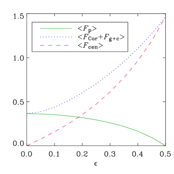
Figure 2: Forces affecting the gas. Average magnitudes of pressure gradient force $F_{\rm p}$, Coriolis force $F_{\rm Cor}$ plus tidal force $F_{\rm g+c}$ and resulting centre-directed force $F_{\rm cen}$ as functions of aspect ratio $\epsilon$. Averages are taken over the vortex boundary. The force unit is $b\varOmega^{2}$.

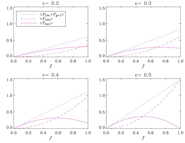
Figure 3: Forces affecting dust as a function of $f$ (dust speed as a fraction of gas speed). Average values of Coriolis force $F_{\rm Cor}$ plus tidal force $F_{\rm g+c}$, necessary centre-directed force to maintain rotation $F_{\rm cen}$ and excess force $F_{\rm exc}$ for different values of aspect ratio $\epsilon$. The force unit is $b\varOmega^{2}$. Averages are taken over the vortex boundary. The forces do not have the same direction, so the two vectors have been added to get the magnitude of the excess force. The excess force converges to the missing pressure gradient force for $f=1$ in all cases.

The pressure gradient force is calculated from Eq. (23) (we consider $z=0$ since the pressure gradient in the $z$-direction is completely balanced by the vertical gravity component),

$$\@vec{F}_{\rm p} = -\@vec{\nabla}h=\pmatrix{\delta^{2}\varOmega^{2}x\cr\delta^{2}\varOmega^{2}\epsilon^{2}y\cr 0}=\delta^{2}\varOmega^{2}\pmatrix{x\cr\epsilon^{2}y\cr 0}$$ (28)

$$= \left(-\frac{3}{1-\epsilon^{2}}+\frac{2\sqrt{3}}{\sqrt{1-\epsilon^{2}}}\right)\varOmega^{2}\pmatrix{x\cr\epsilon^{2}y\cr 0}\,,$$

and the Coriolis force is

$$\@vec{F}_{\rm Cor} = -2\varOmega\hat{\@vec{k}}\times\@vec{u}=-2\varOmega\pmatrix{0\cr 0\cr 1}\times\pmatrix{\epsilon\alpha\varOmega y\cr-\alpha\varOmega x/\epsilon\cr 0}$$ (29)

$$= -2\varOmega\pmatrix{\alpha\varOmega x/\epsilon\cr\epsilon\alpha\varOmega y\cr 0}=-\frac{2\alpha}{\epsilon}\varOmega^{2}\pmatrix{x\cr\epsilon^{2}y\cr 0}$$

$$= -\frac{2\sqrt{3}}{\sqrt{1-\epsilon^{2}}}\varOmega^{2}\pmatrix{x\cr\epsilon^{2}y\cr 0}\,.$$

Note that both forces point perpendicular to the vortex flow. The resulting force,

$$\@vec{F}_{\rm res} = \@vec{F}_{\rm p}+\@vec{F}_{\rm Cor}+\@vec{F}_{\rm g+c}$$ (30)

$$= -\frac{3}{1-\epsilon^{2}}\varOmega^{2}\pmatrix{x\cr\epsilon^{2}y\cr 0}+\pmatrix{3\varOmega^{2}x\cr 0\cr 0}$$

$$= -\frac{3}{1-\epsilon^{2}}\varOmega^{2}\pmatrix{x\cr\epsilon^{2}y\cr 0}-\frac{3}{1-\epsilon^{2}}\varOmega^{2}\pmatrix{(\epsilon^{2}-1)x\cr 0\cr 0}$$

$$= -\frac{3}{1-\epsilon^{2}}\varOmega^{2}\pmatrix{\epsilon^{2}x\cr\epsilon^{2}y\cr 0}=-\frac{3\epsilon^{2}}{1-\epsilon^{2}}\varOmega^{2}\pmatrix{x\cr y\cr 0}\,,$$

points always towards the centre and thus produces the rotating motion. Fig. 2 is a plot of the average values over the vortex boundary of the pressure gradient force, Coriolis force plus tidal force and resulting centre-directed force as a function of $\epsilon$. The force magnitudes have the unit of $b\varOmega^{2}$. As the aspect ratio decreases, the pressure gradient force becomes relatively more important. At $\epsilon=0.5$ the vortex is in equilibrium without any need for a pressure gradients in the $x$-$y$ plane. This pressure-less vortex is exactly the epicyclic vortex considered by Barge & Sommeria (barge+sommeria95 (1995)).

4.2 Forces on the dust

Dust, initially at rest, is accelerated by drag to follow gas around the vortex, but in the beginning with a much smaller velocity. Moving at a fraction $f$ of the gas speed relative to the main shear flow, $\tilde{\@vec{u}}_{\rm d}=f\tilde{\@vec{u}}$, we find for $\@vec{u}_{\rm d}=\tilde{\@vec{u}}_{\rm d}+\@vec{u}^{(0)}$ the expression $\@vec{u}_{\rm d}=f\@vec{u}+(1-f)\@vec{u}^{(0)}$, so dust is subjected to the Coriolis force

$$\@vec{F}_{\rm Cor}=-\frac{2\sqrt{3}}{\sqrt{1-\epsilon^{2}}}f\varOmega^{2}\pmatrix{x\cr\epsilon^{2}y\cr 0}-(1-f)\pmatrix{3\varOmega^{2}x\cr 0\cr 0}\,.$$ (31)

The centre-directed force needed to keep dust spinning around the vortex is proportional to velocity squared, and is therefore reduced by a factor of $f^{2}$ compared to the force needed to keep the gas rotating,

$$\@vec{F}_{\rm cen}=-\frac{3f^{2}\epsilon^{2}}{1-\epsilon^{2}}\varOmega^{2}\pmatrix{x\cr y\cr 0}\,.$$ (32)

The excess force on the dust is then $\@vec{F}_{\rm exc}=\@vec{F}_{\rm Cor}+\@vec{F}_{\rm g+c}-\@vec{F}_{\rm cen}$. In Fig. 3 Coriolis force plus tidal force, centre-directed force needed to maintain the same radius of rotation as the gas and excess force working on the dust are shown as a function of $f$ and for different values of the aspect ratio $\epsilon$. For all value of $\epsilon$ the Coriolis force grows much faster with $f$ than the required centre-directed force. This leads to an excess force directed inwards, which causes dust to spiral inwards. Similar explanations for the dust-trapping mechanism of vortices are given in Tanga et al. (tanga+etal96 (1996)) and Chavanis (chavanis00 (2000)). Already at a few percent of the gas speed, the excess force on the dust is significant. Cyclonic vortices have an outwards directed Coriolis force. They will therefore not be able to concentrate solid particles, but will rather expel them.

The centre-directed force catches up with the Coriolis force at $f=1.0$ for $\epsilon=0.5$, but for higher $\epsilon$ there is still an excess force on the dust at $f=1.0$ of the same magnitude (but opposite direction) as the pressure gradient force affecting the gas. The reason for this is that dust particles are not subjected to the pressure gradient force of gas, so even if dust particles were light enough to quickly become accelerated to match gas velocity, they will feel an extra force inward and thus begin to spiral inwards. The terminal velocity that dust obtains perpendicular to the gas flow, $\@vec{u}_{{\rm d}\perp}^{\rm(ter)}$, is a result of a balance between excess inwards force and drag force,

$$0=-\delta^{2}\varOmega^{2}\pmatrix{x\cr\epsilon^{2}y\cr 0}-\frac{1}{\tau_{\rm s}}\@vec{u}_{{\rm d}\perp}^{\rm(ter)}\,,$$ (33)

which means that

$$\@vec{u}_{{\rm d}\perp}^{\rm(ter)}=-\tau_{\rm s}\delta^{2}\varOmega^{2}\pmatrix{x\cr\epsilon^{2}y\cr 0}\,,$$ (34)

in analogy to the vertical settling of dust towards the mid-plane due to gravity. The time scale for this is quite long,

$$t\sim\frac{1}{\tau_{\rm s}\varOmega^{2}}\,,$$ (35)

considering that the stopping time must be short for the dust to match the velocity of the gas, but if vortices are indeed long-lived, it could prove an important mechanism for trapping dust particles of short stopping time inside vortices of low aspect ratio.

The aspect ratio also has an influence on dust-trapping at low $f$. It is evident from Fig. 3 that the excess force grows faster with $f$ and reaches a higher maximum for high $\epsilon$.

5 Three-dimensional models

The vortex solution of GNG has zero enthalpy outside the vortex, corresponding to zero density through the relation

$$\rho=\rho_{0}\left[(\gamma-1)\frac{h}{c_{\rm s0}^{2}}{\rm e}^{\gamma s/c_{\rm p}}\right]^{1/(\gamma-1)}\,.$$ (36)

This gives rise to a potential problem in three dimensions: hydrostatic equilibrium in the $z$-direction requires

$$-\frac{\partial\varPhi}{\partial z}-\frac{1}{\rho}\frac{\partial P}{\partial z}=0\,,$$ (37)

where

$$\varPhi=\frac{1}{2}\varOmega^{2}z^{2}$$ (38)

is the vertical gravitational potential. This means that the pressure must fall off in the vertical direction, but it must never become negative, so embedding the vortex in a disc of finite density and constant entropy is not possible in the vertical direction.

We use two different ways of modelling the vortices in three dimensions: hot corona and cylindrical vortex.

5.1 Hot corona

Hydrostatic equilibrium in the $z$-direction can be obtained by embedding the vortex in a tenuous gas of high temperature, i.e. a hot corona. In terms of specific enthalpy, Eq. (37) can be written as

$$\frac{\partial\varPhi}{\partial z}=\frac{h}{c_{\mathrm{p}}}\frac{\partial s}{\partial z}-\frac{\partial h}{\partial z}\,.$$ (39)

For a given entropy distribution it is then possible to construct a continuous enthalpy so that hydrostatic equilibrium is obtained. This method is also used by von Rekowski et al. (vReko_etal03 (2003)).

The hot corona simulations are done in a box of size $(L_{x},L_{y},L_{z})/b=(4,32,4)$.

5.2 Cylindrical vortex

Here we extend the vortex to the entire $z$-length of the box. The vortex is then no longer ellipsoidal, but rather cylindrical with an ellipse-shaped cross section. Hydrostatic equilibrium is obtained without use of entropy through

$$\frac{\partial h}{\partial z}=-\frac{\partial\varPhi}{\partial z}=-\varOmega^{2}z,$$ (40)

so $h(z)=-\frac{1}{2}\varOmega^{2}z^{2}+h_{0}$, where $h_{0}$ must be greater than $\frac{1}{2}\varOmega^{2}z_{\rm top}^{2}$ to avoid negative enthalpy anywhere. The cylindrical vortex simulations are done in a box of size $(L_{x},L_{y},L_{z})/b=(4,32,0.4)$. The reason for using a shallower box for the cylindrical vortex is to allow for a smaller $h_{0}$ and thus to have a large density ratio between the vortex and its surroundings (see Sect. 7.3). The minimum enthalpy in the mid-plane is $\frac{1}{2}\varOmega^{2}z_{\rm top}^{2}$, so lowering $z_{\rm top}$ and adopting the minimal enthalpy possible thus leads to a larger density ratio.

In both cases we let dust start with zero initial velocity. Dust density at height $z$ is initialised to be a fraction $r=0.01$ of gas density (see Natta et al. natta+etal00 (2000)) far away from the vortex at the same height. Although the actual value of $r$ does not directly influence dust dynamics, it does influence the amount of back-reaction from dust upon gas.

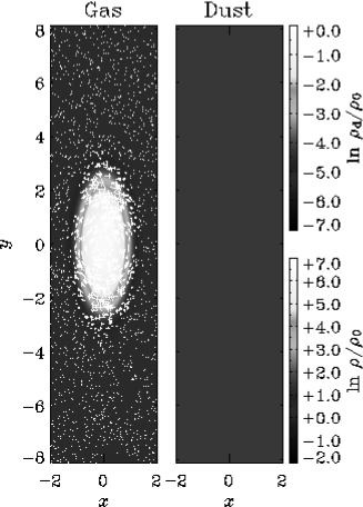
Figure 4: The initial condition in the mid-plane for the hot corona vortex: gas density and gas velocity (left) and the corresponding dust density and velocity (right). The velocity field does not seem to follow the contours of the vortex, but this is because the Kepler velocity has been subtracted.

6 Numerical method and boundary conditions

We simulate the motion of gas and dust in a coordinate frame corotating at the local Keplerian speed. We use the Pencil-Code (Brandenburg & Dobler brandenb+dobler02 (2002)) which uses third order Runge-Kutta time stepping and a sixth order finite-difference scheme in space and employs central finite differences, so the extra cost of recentering a large number of variables between staggered meshes each time step is avoided. The code solves the non-conservative form of the equations (see Brandenburg brandenb03 (2003) for details).

Periodic boundary conditions for velocities, density and specific entropy are used in the $x$- and $y$-directions. The periodic boundary condition in $x$ is appropriately sheared in the shearing sheet approximation. In the $z$-direction we use stress-free boundary conditions, i.e.

$$u_{x,z}=u_{y,z}=u_{z}=s=u_{{\rm d}x,z}=u_{{\rm d}y,z}=u_{{\rm d}z}=0,$$ (41)

where commas denote partial differentiation. Dust and gas densities on the boundaries are fully determined by the equations, but in practice we need to specify values in the ghost zones which is accomplished by extrapolation. We use a resolution of $(n_{x},n_{y},n_{z})=(128,256,128)$ grid points.

7 Results

7.1 Initial conditions and choice of stopping times

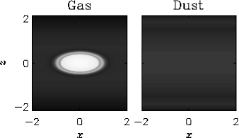
Figure 5: The initial condition in the vertical for the hot corona vortex: gas density (left) and the corresponding dust density (right). Dust density as a function of $z$ is initially 0.01 times gas density in the same height. The density colour scale is the same as in Fig. 4.

The initial condition for gas and dust in the hot corona model is plotted in Fig. 4 (mid-plane , only one fourth of the $y$-length of the box is shown) and Fig. 5 ($x$-$z$ plane). We choose an aspect ratio of $\epsilon=0.4$ since we expect dust-trapping to be most efficient for vortices of high aspect ratio. The transition from vortex to surroundings has been smeared out both in density and velocity field. We have experienced that the simulations run better when abrupt transitions are smoothed out. The dust is initially at rest. In all plots of velocity fields we use the Kepler-subtracted velocities $\tilde{\@vec{u}}$ and $\tilde{\@vec{u}}_{\rm d}$.

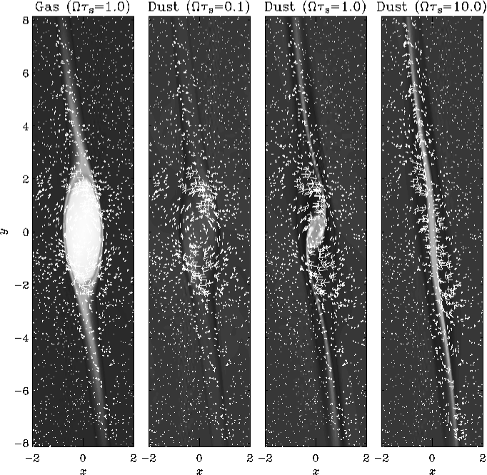
Figure 6: Gas and dust in the mid-plane for the hot corona after one orbit. Gas density and velocity field for the three values of $\varOmega\tau_{\rm s}$ are indistinguishable, so only $\varOmega\tau_{\rm s}=1.0$ is shown. The other three plots show dust density and dust velocity field after one orbit for $\varOmega\tau_{\rm s}=0.1$, $\varOmega\tau_{\rm s}=1.0$ and $\varOmega\tau_{\rm s}=10.0$ respectively. The dust velocity field of $\varOmega\tau_{\rm s}=0.1$ is very similar to that of the gas, due to the short stopping time. For $\varOmega\tau_{\rm s}=1.0$ there is a strong convergence towards the interior of the vortex, whereas for $\varOmega\tau_{\rm s}=10.0$ only a slight density increase in a narrow region that extends from the vortex along the shear is seen. The density colour scales are the same as in Fig. 4.

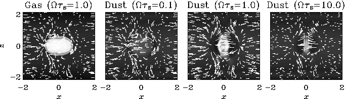
Figure 7: Gas and dust in the $x$-$z$ plane for the hot corona case after one orbit. Gas density and velocity field for the three values of $\varOmega\tau_{\rm s}$ are indistinguishable, so only $\varOmega\tau_{\rm s}=1.0$ is shown. The other three plots show dust density and dust velocity field after one orbit for $\varOmega\tau_{\rm s}=0.1$, $\varOmega\tau_{\rm s}=1.0$ and $\varOmega\tau_{\rm s}=10.0$ respectively. For $\varOmega\tau_{\rm s}=0.1$ dust is so strongly coupled to gas that the velocity fields are very similar, whereas $\varOmega\tau_{\rm s}=1.0$ shows strong convergence of dust in the interior of the vortex. For $\varOmega\tau_{\rm s}=10.0$ dust is not as affected by gas motion, although strong motions move dust around the vortex and upwards. Velocities are exaggerated about 10 times compared to Fig. 6. The density colour scales are the same as in Fig. 4.

We have run hot corona simulations for three different values of the stopping time: $\varOmega\tau_{\rm s}=0.1$ (dust completely coupled to gas), $\varOmega\tau_{\rm s}=1.0$ (dust semi-coupled to gas) and $\varOmega\tau_{\rm s}=10.0$ (dust almost not coupled to gas). This corresponds to rocks of sizes respectively $a_{\rm s}=10\leavevmode\nobreak\ \rm{cm}$, $a_{\rm s}=100\leavevmode\nobreak\ \rm{cm}$ and $a_{\rm s}=1000\leavevmode\nobreak\ \rm{cm}$, respectively. For the minimum-mass nebula of Cuzzi et al. (cuzzi+etal93 (1993)) the mean free path is $\lambda=(r/{\rm AU})^{11/4}\,{\rm cm}$. This means that we must, strictly speaking, go beyond $r=10\,{\rm AU}$ for the largest particles to be in the Epstein regime. For $a_{\rm s}=10\leavevmode\nobreak\ \rm{cm}$ and $a_{\rm s}=100\leavevmode\nobreak\ \rm{cm}$ the Epstein drag law is valid already before $r=5\,{\rm AU}$. The range of dust radii considered is expected for the largest agglomorations of sticking dust particles after having reached the mid-plane, according to Weidenschilling & Cuzzi (weidenschilling+cuzzi93 (1993)) who model how dust particles falling towards the mid-plane stick to each other in a turbulent protoplanetary disc. Larger sizes are prohibited by the turbulence in the disc.

The cylindrical vortex was only run for $\varOmega\tau_{\rm s}=1.0$, since we are mostly interested in whether it is a valid 3D vortex solution. We follow the evolution of gas and dust for a full Kepler orbit $t_{\rm max}=2\pi/\varOmega$ (which is not quite a full rotation of the vortex, see Fig. 1).

7.2 Viscosity parameters

For the hot corona model we are able to run for a whole orbit with a viscosity of $\nu=\nu_{\rm d}=2\cdot 10^{-4}$ and a shock viscosity of $c_{\rm shock}=2$. This corresponds to a mesh Reynolds number of

$$\mbox{Re}_{\rm mesh}=\max(|\tilde{\@vec{u}}|)\max(\delta x,\delta y,\delta z)/\nu\approx 625\,.$$ (42)

Thus, since $\mbox{Re}_{\rm mesh}$ is rather large, the viscosity $\nu$ is almost everywhere unimportant, and most dissipations occurs through the shock viscosity (not included in the expression for $\mbox{Re}_{\rm mesh}$), but this affects only convergent flow regions and not the vortical parts of the flow. This can be seen from the following consideration.

The Laplacian of $\tilde{\@vec{u}}$ can be written $\@vec{\nabla}^{2}\tilde{\@vec{u}}=-\@vec{\nabla}\times\@vec{\nabla}\times\tilde{\@vec{u}}+\@vec{\nabla}\@vec{\nabla}\cdot\tilde{\@vec{u}}$. Using this we can rewrite the expression for the viscous force as

$$\frac{\@vec{F}_{\rm visc}}{\rho}=\nu\left(-\@vec{\nabla}\times\tilde{\@vec{\omega}}+2\@vec{\mathsf{S}}\cdot\@vec{\nabla}\ln\rho\right)+({\textstyle\frac{4}{3}}\nu+\zeta)\@vec{\nabla}\@vec{\nabla}\cdot\tilde{\@vec{u}}\,,$$ (43)

where $\tilde{\@vec{\omega}}=\@vec{\nabla}\times\tilde{\@vec{u}}$ is the vorticity of the flow. This shows that the kinematic shear viscosity works as a drain for vorticity in regions where the vorticity changes, whereas shock viscosity only affects regions of convergence in the velocity field.

At the boundary between vortex and surroundings the vorticity changes abruptly, and we have experienced vortices dissolving rapidly when using too high a viscosity. We stress that this is a purely numerical issue, and that real physical viscosity is many orders of magnitude lower than the viscosity we use here.

For the cylindrical vortex we had to use a viscosity of $\nu=\nu_{\rm d}=10^{-2}$ and a shock viscosity of $c_{\rm shock}=4$. The reason for these higher viscosities is that the cylindrical vortex does not have as large a density ratio as the hot corona vortex, so it takes more viscosity to keep the vortex intact on the boundary.

7.3 Lifetime of vortices

When using a realistic disc background density we have experienced the vortices breaking up at the local sound speed at the vortex boundary. This we believe is caused by the term $\@vec{\nabla}\cdot\tilde{\@vec{u}}$ in the continuity equation (3). Although the initial condition has $\@vec{\nabla}\cdot\tilde{\@vec{u}}=0$ analytically, this is not necessarily valid numerically. Calculating the spatial derivatives of the velocity field on a Cartesian coordinate grid yields $\@vec{\nabla}\cdot\tilde{\@vec{u}}\neq 0$ over a few mesh-points (due to the order of the numerical derivatives) around the vortex boundary. The result is the depletion of density at the NW and SE corners of the vortex, and increase of density at the NE and SW corners. We find that we can alleviate this problem by having a large density contrast between the vortex and its exterior [as also suggested by the GNG vortex solution, cf. Eq. (23)]. We also find that shock viscosity helps to reduce this problem.

For the hot corona, we plot in Fig. 6 gas density, gas velocity, dust density and dust velocity in the mid-plane after one orbit. The gas configuration is indistinguishable between different values of $\varOmega\tau_{\rm s}$, indicating that there is very little back-reaction on the gas, so gas density and velocity field are only shown for $\varOmega\tau_{\rm s}=1.0$.

The vortex is evidently still in place, although the outer parts have been sheared away to form long tails in the direction of the shear. In Fig. 7 gas density and dust density in the $x$-$z$ plane are plotted. Again we see that the vortex is still in place after one orbit. We conclude from this that the hot corona vortex solution is valid even in the presence of shear.

The status of the cylindrical vortex after one orbit is shown in Fig. 8. In the mid-plane it seems to be more disrupted than the hot corona vortex, possibly due to the smaller density ratio between the vortex and its surroundings. A vertical cut (not shown) reveals that the original stratification of the vortex is almost intact, which implies that the cylindrical vortex model is also a valid one.

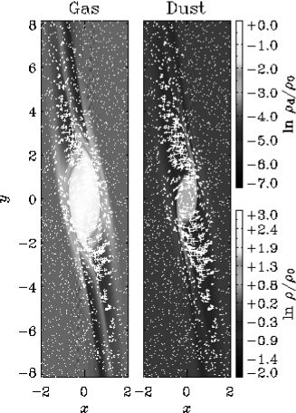
Figure 8: Gas and dust in the mid-plane for the cylindrical vortex after one orbit, $\varOmega\tau_{\rm s}=1.0$. The vortex is close to breaking up: two arcs of matter are being expelled at the NE and SW corners. Note that the density contrast between the vortex and its surroundings is much smaller than for the hot corona vortex, and that the gas density colour scale is different from the hot corona’s.

To test the lifetimes of vortices beyond one orbit we have run low-resolution simulations ($64\times 128\times 64$) for different values of the viscosity $\nu$. Since the major effect of viscosity takes place at the vortex boundary where the velocity (and thus the mass flux) is highest, we plot the maximum mass flux $(\rho u)_{\rm max}$ in the box as a function of time measured in orbits in Fig. 9. The lifetime is obviously very dependent on the viscosity, with lower viscosities leading to longer-living vortices. A low viscosity, on the other hand, also leads to more chaotic development in maximum mass flux, probably due to too high a mesh Reynolds number.

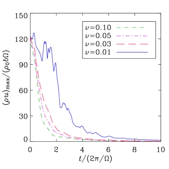
Figure 9: Maximum mass flux in the box as a function of time (measured in orbits) for different values of the viscosity $\nu$. A low viscosity obviously increases the lifetime of a vortex. On the other hand a low viscosity also leads to more chaotic development in $(\rho u)_{\rm max}$, indicating that the mesh Reynolds number may become too high.

7.4 Evolution of dust density

Also shown in Figs 6 and 7 is the evolution of dust density. As expected, the most efficient dust-trapping occurs when dust and gas are semi-coupled with $\varOmega\tau_{\rm s}=1.0$, where the increase in dust density inside the vortex is from an initial $\ln\rho_{\rm d}/\rho_{0}=-4.18$ to a maximum of $\ln\rho_{\rm d}/\rho_{0}=-1.34$ after one orbit, a 17 times increase in density. A depletion of dust in the outer parts of the vortex is also seen. We believe this is where the trapped dust has been taken from. There is a strong convergence in the dust velocity field both in the mid-plane and in the $x$-$z$ plane.

For $\varOmega\tau_{\rm s}=0.1$ dust is accelerated to match the gas velocity very quickly (compared to an orbit) and only a very modest increase in dust density is seen inside the vortex. This could be the slow settling of dust that was discussed in Sect. 4, which should here happen on a time scale of about $10/\varOmega$. The velocity field of Fig. 7 does however not show any convergence inside the vortex. But according to Eq. (34) the inwards drift could happen with a velocity of only $u^{\rm(ter)}/(b\varOmega)\approx\tau_{\rm s}\varOmega\delta^{2}\approx 0.02$ for $\varOmega\tau_{\rm s}=0.1$ and $\epsilon=0.4$, a contribution in peril of drowning completely in the erratic motions present after one orbit, although it could still be present underneath it. A narrow region of dust depletion is apparent around the edge of the vortex. This may be caused by the slow inwards drift of dust (its radius of $\sim 0.1$ is comparable to the expected $0.02\cdot 2\pi=0.13$), although it is not clear why the $\varOmega\tau_{\rm s}=10.0$ vortex should have a region of similar depletion. In Fig. 10 we show gas and dust configurations of the $\varOmega\tau_{\rm s}=0.1$ vortex after 1.5 orbits. The dust-depleted region on the vortex boundary has obviously not become wider, nor has the dust density inside the vortex increased. Gas density has changed a lot. The vortex now has a pronounced tilt in the NW-SE direction, and the shear tails have grown more massive in density. The reason why we do not see any dust-trapping may then very well be that vortex dynamics completely dominates over the slow inwards drift of dust, rendering the mechanism for trapping short stopping time dust particles useless.

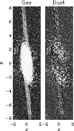
Figure 10: Gas and dust density and velocity fields after 1.5 orbits for $\varOmega\tau_{\rm s}=0.1$. Comparing with Fig. 6 (plot number two from left) there is no apparent widening of the dust-depleted region on the vortex boundary, nor has the dust density increased inside the vortex. The colour scale is the same is in Fig. 4.

For a stopping time parameter of $\varOmega\tau_{\rm s}=10.0$ dust is so unaffected by gas that only a slight density increase is seen. The increase has occurred in a narrow region that extends from the vortex along the shear. This may be the dust-trapping mechanism that here takes place so slowly that dust is sheared away faster than the vortex can trap it.

7.5 Back-reaction on gas

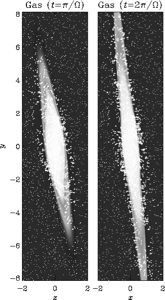
Figure 11: Gas configuration after half an orbit (left) and after a whole orbit (right) for a dust-to-gas ratio of the order of $1$ inside the vortex ($100$ in the disc). Velocities are reduced by around a factor of 5 compared to the initial condition. Gas is forced to follow the converging dust, and that leads to the destruction of the vortex. The colour scale is the same is in Fig. 4.

One very important issue regarding vortices is how they are affected by the dust they trap. Vertical dust-settling at the same time increases dust density in the mid-plane, and at one point dust density in the vortex is expected to become comparable to gas density. Then the back-reaction on gas becomes important in the dynamics of the gas, Eq. (13).

As mentioned in Sect. 7.3 the reason why gas develops similarly in our simulations for all values of stopping time is that the back-reaction on the gas from dust is negligible. This is caused by two things: a dust-to-gas ratio of $0.01$ is not very high, and furthermore this ratio only applies in the disc, whereas we know that gas density in the vortex is very much higher, giving an even lower dust-to-gas ratio there. The back-reaction would eventually become much bigger if we allowed for vertical settling of dust.

To test when the back-reaction from dust becomes important we have run the $\varOmega\tau_{\rm s}=1.0$ and $\varOmega\tau_{\rm s}=10.0$ vortices with higher values of the dust-to-gas ratio. In Fig. 11 we plot the gas configuration of the $\varOmega\tau_{\rm s}=1.0$ vortex when the dust-to-gas ratio is $100$. At this point dust density becomes comparable to gas density inside the vortex. We see that the vortex is not only affected by dust drag, but that it is even almost completely destroyed after one orbit. When dust converges inside the vortex, it will drag gas along with it, in this way destroying the vortex.

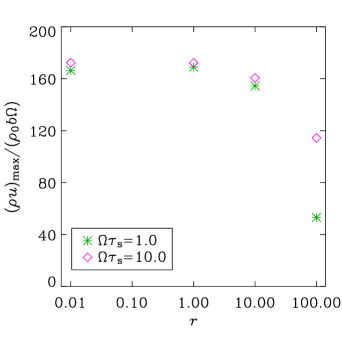
Figure 12: The maximum mass flux in the box after one orbit when varying the dust-to-gas ratio from 0.01 to 100, the latter corresponding to a dust-to-gas ratio of unity inside the vortex. Points are shown for both $\varOmega\tau_{\rm s}=1.0$ and $\varOmega\tau_{\rm s}=100.0$. The best dust-trapper, $\varOmega\tau_{\rm s}=1$, is also the best at destroying the vortex, due to the trapped dust dragging gas along with it.

The maximum mass flux in the box after one orbit as a function of dust-to-gas ratio in the disc is shown in Fig. 12. Already when the dust-to-gas ratio in the disc is $10$ (corresponding to around $0.1$ in the vortex), the back-reaction becomes important. The $\varOmega\tau_{\rm s}=1.0$ vortex is best at destroying the vortex at all dust-to-gas ratios.

8 Conclusions

In this paper we have explored the suggestion of Barge & Sommeria (barge+sommeria95 (1995)) of trapping dust particles in anticyclonic vortices. In recent years the vortex theory has gained increasing popularity as a site for planetesimal formation.

To our knowledge this is the first time the dust-trapping mechanism has been explored in three dimensions and with a freely developing gas velocity field and density. We use two ways to model the vortices in three dimensions, and we have shown that both models survive well for at least one orbit. It is conceivable that long life times are possible at yet higher resolution when the viscosity can be smaller. We have also shown the dust-trapping capabilities of vortices. For both vortex models dust-trapping is very efficient when dust and gas are semi-coupled, whereas too little or too much coupling gives no significant dust-trapping. The most efficiently trapped solid particles have a radius of 100 centimetres. This may be in some conflict with meteoritic evidence, where chondrules (the building blocks of the most pristine meteorites) are typically up to 1 millimetre in radius. But meteorites on Earth are found to originate in the asteroid belt and should therefore not necessarily say anything about the make up of pristine material in the outer Solar System.

Our two three-dimensional models both have a large density contrast between the vortex and the surrounding disc. A model with a realistic disc density profile could be obtained by using coordinates more natural to the vortex flow, such as elliptical coordinates. This would also require a version of the shearing sheet approximation adapted to new coordinates (for spherical coordinates there exists the shearing disc approximation of Klahr & Bodenheimer klahr+bodenheimer03 (2003)). Alternatively, and probably better, a global solution to the Euler and continuity equations with a gradual transition from vortex to surrounding Kepler flow could be used. Such global solutions have been found to the Euler equation alone (Chavanis chavanis00 (2000), de la Fuente Marcos & Barge fuente+barge01 (2001)), but none to our knowledge satisfy the continuity equation.

The role of vortices as high pressure regions seems hitherto unexplored. Short stopping time solid particles forced to match gas speed around the vortex will feel an additional pull inwards. The drift is similar to the vertical settling of dust towards the mid-plane. Although this happens on quite a long time scale compared to the conventional dust-trapping time, it seems a viable mechanism for catching short stopping time dust particles, provided vortices live long enough. Unfortunately our simulations do not show this mechanism at work, but rather that vortex and gas dynamics completely dominates over this effect, even if it is present.

It will be necessary to address the questions as to what causes such vortices in the first place. It seems plausible that anticyclonic vortices form as a relic after the disc turbulence in the disc has died out (Bracco et al. bracco+etal98 (1998); bracco+etal99 (1999)). This idea is particularly attractive, because the absence of turbulence may be an important prerequisite for allowing dust to settle to the mid-plane. Other suggestions include baroclinic instabilities (Klahr & Bodenheimer, klahr+bodenheimer03 (2003)), the anisotropic kinetic alpha-effect (von Rekowski et al. vReko_etal99 (1999)), and perhaps even the possibility of brown dwarf encounter (Willerding willerding02 (2002)). The original work by GNG was inspired by numerical results of the Papaloizou-Pringle instability, but this instability is not available in a thin Kepler disc with $q=3/2$. Stability analysis in GNG suggested that the vortices suffer from numerous linear instabilities, so the survival of the vortices in 3D for at least one orbit seems surprising. In any case, it will be important to relax the need for implementing vortices as initial conditions and rather try to get them automatically under realistic conditions.

The photometric observations of the protostar KH15D has been interpreted by Barge & Viton (barge+viton03 (2003)) as a giant dusty vortex rotating at a distance of 0.2 AU from the star and covering 120^∘ of the orbit. Such a large vortex is beyond the validity of the shearing sheet approximation (where the curvilinearity of the disc is neglected) and requires a global hydrodynamical disc simulation to examine its stability and creation. If the vortex interpretation is correct, it could be the opening of a new era of observational vortex research. The next generation of telescopes such as ALMA (see Wolf & Klahr wolf+klahr02 (2002)) will be able to probe protoplanetary discs all over the sky for evidence of vortex activity. This will be the ultimate test of whether the research done so far in the field has been just an intellectual exercise, or if planets do indeed form partially as a result of long-lived vortices. This would make the vortex dust-trapping theory an important step in planet formation. Perhaps we owe the existence of our own planet to vortices that were present in the solar nebular 4.6 billion years ago.

Appendix A Derivation of vortex solution

In this Appendix we show how to construct an elliptical velocity field and an appropriate corresponding enthalpy that satisfies Eqs. (18) and (19). We start out by proposing that the velocity field Eqs. (20)–(22) is indeed a solution, provided that the aspect ratio and the angular velocity fulfil certain criteria. This velocity field is divergence-free and has no $z$-component. It can then be written as the curl of a stream function $\@vec{\varPsi}$ with only a $z$-component, $\@vec{u}=\@vec{\nabla}\times\@vec{\varPsi}$.

Given the velocity field $\@vec{u}$ one can attempt to construct an enthalpy such that the flow is steady with $\partial\@vec{u}/\partial t=\@vec{0}$. This implies that

$$\@vec{\nabla}h=\varOmega^{2}(3\@vec{x}-\@vec{z})-2\@vec{\varOmega}\times\@vec{u}-(\@vec{u}\cdot\@vec{\nabla})\cdot\@vec{u}\,.$$ (44)

The tidal force term and the vertical gravity term on the right hand side are obviously gradient terms. The same is true for the Coriolis term since

$$\hat{\@vec{k}}\times\@vec{u}=\pmatrix{0\cr 0\cr 1}\times\pmatrix{\partial\varPsi/\partial y\cr-\partial\varPsi/\partial x\cr 0}=\pmatrix{\partial\varPsi/\partial x\cr\partial\varPsi/\partial y\cr 0}=\@vec{\nabla}\varPsi\,.$$ (45)

We are now left with (ignoring the integration constants for now)

$$\@vec{\nabla}h=\@vec{\nabla}({\textstyle\frac{3}{2}}\varOmega^{2}x^{2}-{\textstyle\frac{1}{2}}\varOmega^{2}z^{2}-2\varOmega\varPsi)-(\@vec{u}\cdot\@vec{\nabla})\cdot\@vec{u}\,.$$ (46)

The advective term $(\@vec{u}\cdot\@vec{\nabla})\@vec{u}$ is a bit more tricky to put in gradient form. It can be done by applying the vector identity

$$(\@vec{u}\cdot\@vec{\nabla})\@vec{u}=\@vec{\nabla}({\textstyle\frac{1}{2}}\@vec{u}^{2})-\@vec{u}\times(\@vec{\nabla}\times\@vec{u})\,.$$ (47)

The first term on the right hand side comes out on gradient form. The second can be calculated by noting that

$$\@vec{\nabla}\times\@vec{u}\equiv\@vec{\omega}=\pmatrix{0\cr 0\cr-\partial^{2}\varPsi/\partial x^{2}-\partial^{2}\varPsi/\partial y^{2}}\,,$$ (48)

where the vorticity $\@vec{\omega}$ of the flow is introduced. The second term on the right hand side of Eq. (47) can now be rewritten as

$$\@vec{u}\times(\@vec{\nabla}\times\@vec{u})=\pmatrix{\partial\varPsi/\partial y\cr-\partial\varPsi/\partial x\cr 0}\times\pmatrix{0\cr 0\cr\omega}=-\omega\@vec{\nabla}\varPsi\,.$$ (49)

If the vorticity is constant and independent of the spatial coordinates, this can be written

$$\@vec{u}\times(\@vec{\nabla}\times\@vec{u})=\@vec{\nabla}(-\omega\varPsi)\,.$$ (50)

The gradient of the enthalpy can now be written entirely as a sum of gradient terms,

$$\@vec{\nabla}h=\@vec{\nabla}({\textstyle\frac{3}{2}}\varOmega^{2}x^{2}-{\textstyle\frac{1}{2}}\varOmega^{2}z^{2}-2\varOmega\varPsi-{\textstyle\frac{1}{2}}\@vec{u}^{2}-\omega\varPsi)\,.$$ (51)

This is easily integrated to give

$$h={\textstyle\frac{3}{2}}\varOmega^{2}x^{2}-{\textstyle\frac{1}{2}}\varOmega^{2}z^{2}-(2\varOmega+\omega)\varPsi-{\textstyle\frac{1}{2}}\@vec{u}^{2}+{\rm const}\,,$$ (52)

where all the integration constants are collected in just one constant.

In order to calculate the enthalpy of the flow given by Eqs. (20)–(22) we need to know also the stream function and the vorticity of the flow. The magnitude of the stream function is

$$\varPsi={\textstyle\frac{1}{2}}\left(\frac{1}{\epsilon}x^{2}+\epsilon y^{2}\right)\varOmega^{\prime}\,,$$ (53)

and the vorticity has the magnitude

$$\omega=-\frac{\partial^{2}\varPsi}{\partial x^{2}}-\frac{\partial^{2}\varPsi}{\partial y^{2}}=-\left(\frac{1}{\epsilon}+\epsilon\right)\varOmega^{\prime}\,.$$ (54)

This is a constant, and Eq. (52) can therefore be applied. To simplify the calculations we write the enthalpy as $h(x,y,z)=h_{x}(x)+h_{y}(y)+h_{z}(z)$ (as there are no mixed terms). For $h_{x}$ we get

$$h_{x}=({\textstyle\frac{3}{2}}\varOmega^{2}-\varOmega\frac{1}{\epsilon}\varOmega^{\prime}+{\textstyle\frac{1}{2}}\varOmega^{\prime 2})x^{2}\equiv Bx^{2}\,;$$ (55)

similarly for $h_{y}$,

$$h_{y}=(-\varOmega\epsilon\varOmega^{\prime}+{\textstyle\frac{1}{2}}\varOmega^{\prime 2})y^{2}\equiv Ay^{2}\,;$$ (56)

and for $h_{z}$,

$$h_{z}=-{\textstyle\frac{1}{2}}\varOmega^{2}z^{2}\equiv Cz^{2}\,.$$ (57)

Now the enthalpy can be written as $h=Bx^{2}+Ay^{2}+Cz^{2}$. This can be done for any angular velocity $\varOmega^{\prime}$ of the vortex.

An equilibrium flow solution must also have $\partial\rho/\partial t=0$ everywhere. The continuity equation Eq. (19) can be rewritten as

$$\frac{\partial\rho}{\partial t}+\@vec{\nabla}\cdot(\rho\@vec{u}) = \frac{\partial\rho}{\partial t}+\rho(\@vec{\nabla}\cdot\@vec{u})+\@vec{u}\cdot\@vec{\nabla}\rho$$ (58)

$$= \frac{\partial\rho}{\partial t}+\@vec{u}\cdot\@vec{\nabla}\rho=0\,,$$

since the velocity field has $\@vec{\nabla}\cdot\@vec{u}=0$. This means that the gradient of the density must everywhere be perpendicular to the flow, since $\@vec{u}\cdot\@vec{\nabla}\rho$ must be equal to zero. In the absence of an entropy gradient the gas is barotropic, so $\@vec{\nabla}\rho$ and $\@vec{\nabla}h$ are parallel, and therefore $\@vec{u}\cdot\@vec{\nabla}h=0$. This means that the contours of enthalpy must be ellipses with the same aspect ratio as the vortex.

For the enthalpy given by $h(x,y,z)=Bx^{2}+Ay^{2}+Cz^{2}$, where the coefficients are specified in Eqs. (55)–(57), and a velocity field given by Eqs. (20)–(22), this leads to

$$\frac{A}{B}=\epsilon^{2}=\frac{-\varOmega\epsilon\varOmega^{\prime}+\frac{1}{2}\varOmega^{\prime 2}}{\frac{3}{2}\varOmega^{2}-\varOmega\frac{1}{\epsilon}\varOmega^{\prime}+\frac{1}{2}\varOmega^{\prime 2}}\,,$$ (59)

which implies that

$${\textstyle\frac{3}{2}}\varOmega^{2}\epsilon^{2}-\varOmega\epsilon\varOmega^{\prime}+{\textstyle\frac{1}{2}}\epsilon^{2}\varOmega^{\prime 2} = -\varOmega\epsilon\varOmega^{\prime}+{\textstyle\frac{1}{2}}\varOmega^{\prime 2}$$

$$\Rightarrow\varOmega^{\prime} = \frac{\sqrt{3}\epsilon\varOmega}{\sqrt{1-\epsilon^{2}}}\equiv\alpha\varOmega\,.$$ (60)

This solution requires that $0\leqslant\epsilon<1$. Negative $\epsilon$ in the same range in principle also give solutions, but the enthalpy and velocity field do not change since $\epsilon$ only enters as $\epsilon^{2}$ when $\varOmega^{\prime}$ is inserted. The parameters $B$, $A$ and $C$ are

$$B = -{\textstyle\frac{1}{2}}\varOmega^{2}\left(-\frac{3}{1-\epsilon^{2}}+\frac{2\sqrt{3}}{\sqrt{1-\epsilon^{2}}}\right)$$ (61)

$$A = -{\textstyle\frac{1}{2}}\varOmega^{2}\left(-\frac{3}{1-\epsilon^{2}}+\frac{2\sqrt{3}}{\sqrt{1-\epsilon^{2}}}\right)\epsilon^{2}$$ (62)

$$C = -{\textstyle\frac{1}{2}}\varOmega^{2}$$ (63)

For $0.5<\epsilon<1$ the coefficients $B$ and $A$ are positive, resulting in a region of low pressure with a clockwise rotation around it, contrary to the counter-clockwise rotation around low-pressures on Earth. As in the GNG paper we focus only on $0\leqslant\epsilon\leqslant 0.5$. Here $B$ and $A$ are negative, and the result is a high-pressure region. Defining $\delta^{2}=-\frac{3}{1-\epsilon^{2}}+\frac{2\sqrt{3}}{\sqrt{1-\epsilon^{2}}}$ and requiring that the enthalpy vanish on the vortex boundary gives

$$h={\textstyle\frac{1}{2}}\delta^{2}\varOmega^{2}(b^{2}-x^{2}-\epsilon^{2}y^{2})-{\textstyle\frac{1}{2}}\varOmega^{2}z^{2}\,.$$ (64)