Abstract: We present a detailed statistical study of the observed anisotropy in radio polarizations from distant extragalactic objects. This anisotropy was earlier found by Birch (1982) and reconfirmed by Jain & Ralston (1999) in a larger data set. A very strong signal was seen after imposing the cut $|RM-\overline{RM}|>6$ rad/m², where $RM$ is the rotation measure and $\overline{RM}$ its mean value. In this paper we show that there are several indications that this anisotropy cannot be attributed to bias in the data. We also find that a generalized statistic shows a very strong signal in the entire data without imposing the RM dependent cut. Finally we argue that an anisotropic background pseudoscalar field can explain the observations.

Keywords: Polarization, magnetic fields, galaxies: active, galaxies: high-redshift, cosmology: miscellaneous, elementary particles

1. Introduction

Polarizations of radio waves from extragalactic sources undergo Faraday Rotation upon propagation through galactic magnetic fields. This effect provides very useful information about astrophysical magnetic fields (Zeldovich, Ruzmaikin & Sokoloff 1983, Vallée 1997). The amount of rotation is proportional to the magnetic field component parallel to the direction of propagation of the wave and to the square of the wavelength $\lambda$. The observed orientation $\theta(\lambda)$ of the linearly polarized component of the electromagnetic wave can therefore be written as,

$$\theta(\lambda^{2})=\chi+\left(RM\right)\lambda^{2}$$ (1)

where the slope, called Faraday Rotation Measure ($RM$), depends linearly on the line integral of the parallel component of the magnetic field along the direction of propagation of the wave and $\chi$ is the intercept, also called the intrinsic position angle of polarization, $IPA$.

The observed polarization angle $\chi$, after the effect of Faraday rotation is taken out of the data, is observed to be dominantly aligned perpendicular to the orientation axis of the galaxy. Let $\psi$ denote the orientation angle of the galaxy. Then the offset angle $\beta=\chi-\psi$ is found to be approximately equal to $\pi/2$ for most of the sources, i.e. the distribution of $\beta$ over a large sample of sources is found to peak at $\beta\approx\pi/2$. Besides this dominant trend, a smaller peak is also found at $\beta\approx 0$. This suggests the existence of two populations, some with polarization position angles parallel and others perpendicular to the galaxy axis.

In $1982$, Birch empirically observed an angular anisotropy in the offset angle $\beta$, using a data set of $137$ points. Birch’s statistics were questioned by Phinney & Webster (1983) and it was pointed out that the significance of Birch’s result can be significantly reduced if the experimental errors in $\beta$ are taken into consideration. Phinney & Webster (1983) also suggested that the signal observed by Birch might result from the presence of bias in data. Kendall & Young (1984) further investigated Birch’s claim of cosmic anisotropy with more sophisticated statistics and using an updated version of Birch’s data. They found that the statistics were not consistent with isotropy at $99.9$% confidence level. Later Bietenholz & Kronberg (1984) repeated the calculations using single-number correlation test statistic, originally proposed by Jupp & Mardia (1980). This statistic also showed strong evidence of anisotropy in Birch’s data with a confidence level of $99.98$%. They went on to create an independent set of 277 points which, however, showed no signal of anisotropy. This lead to a dismissal of Birch’s results but left unresolved the puzzling fact that his data had contained a signal of anisotropy at such a high level of statistical significance.

The possible existence of anisotropy in radio polarizations was reanalysed by Jain & Ralston (1999). The authors collected an independent set of $361$ points from all the available catalogues. This set included $\beta$ values for 29 sources which were contained only in the Birch’s compilation. Jain & Ralston (1999) also considered the data set of 332 sources obtained after deleting these 29 objects. The authors found that both the data sets showed a statistically significant signal of anisotropy. The observed signal can be expressed as follows,

$$2\beta-\pi\approx\mbox{\boldmath$\Lambda$}\cdot\mbox{\boldmath$R$}$$ (2)

where $R$ is a unit vector in the direction of the source. The vector $\Lambda$ represents the three parameters of this fit and points in the prefered direction of this dipole anisotropy. The unit vector $\hat{\Lambda}$ controls the distribution of $(2\beta-\pi)$ on the dome of the sky such that it is predominantly positive in the direction of the axis while it is predominantly negative in the opposite direction.

Jain & Ralston (1999) tested the isotropy as null hypothesis using Maximum Likelihood analysis by taking into account the transformation property of $\beta$. A typical null distribution for angular variables is the von Mises (vM) distribution

$$vM(\theta)=const\times e^{k\cos(\theta)}$$ (3)

where $k$ is a constant and $\theta$ is the angular parameter which is taken here to be $2\beta$. The factor 2 arises since $\beta$ refers to the polarization angle and $\beta+\pi$ is identified with $\beta$ (Ralston & Jain 1999). The joint distribution of the angle $\beta$ and source positions was taken to be of the form

$$f(2\beta)C(2\beta,{\bf R})h({\bf R})\ ,$$

where $f(2\beta)$ is the marginal distribution of $\beta$ which is assumed to be the von Mises, $h({\bf R})$ is the angular distribution of the sources and the correlation ansatz is taken to be of the form,

$$C(2\beta,{\bf R})=\exp\left[\mbox{\boldmath$\lambda$}\cdot{\bf R}\sin{2\beta}\right]$$ (4)

Here $\lambda$ represent the three parameters of the correlation ansatz. An alternate distribution, obtained by replacing

$$2\beta\rightarrow\Omega(\beta)=2\beta+\nu sin2\beta$$ (5)

was also considered by Jain & Ralston (1999) since it was found to provide a better null fit to the data. The fit selected a negative value of the parameter $\nu\approx-1$ which leads to a more sharply peaked distribution in comparison to the von Mises. Such a sharply peaked function is also justified by the distribution of polarizations obtained under the assumption that the electric field components of the electromagnetic wave are normally distributed (Sarala & Jain 2001, 2002).

Likelihood analysis showed a strong signal of anisotropy using the transformation 5 in the joint distribution 4. The strongest signal was obtained after making the cut on the rotation measures so as to eliminate the data with RM in the range $|RM-\overline{RM}|\leq 6$, where $\overline{RM}=6\ rad/m^{2}$ is the mean value of the rotation measure over the data sample. In fig. 1 we show the histogram of the rotation measures for the 332 sources. It is found that the peak position as well as the mean value of RM is shifted from zero and lies approximately at $6\ rad/m^{2}$. This is somewhat unexpected since for a large unbiased sample we would expect the peak value of $RM$ to be zero. Even for a larger data sample compiled in Broten, MacLeod & Vallee (1988) we find similar distribution with peak position as well as the mean and median of the rotation measures shifted from zero towards positive values. The cut on RM, therefore, removes points lying close to the central peak in the distribution. The statistical significance of the signal after this cut was found to be approximately 0.06%, i.e. the probability that the correlation seen in data might arise in a random sample is given by $P=0.06$%. The unit vector $\hat{\lambda}$ after making the cut $|RM-\overline{RM}|>6$ was found to be (Jain & Ralston 1999)

$$\mbox{\boldmath$\hat{\lambda}$}=[(0\ h,9\ m)\pm(1\ h,0\ m),-1^{o}\pm 15^{o}]\$$ (6)

in the B1950 coordinate system.

Similar results were obtained by using the Jupp and Mardia correlation coefficient. In this case the authors (Jain & Ralston 1999) found the correlation between $\sin(2\beta-sin2\beta)$ and the angular position vector of the source. The parameter $\nu$ in Eq. 5 was set equal to $-1$ since the likelihood analysis generally prefered a value between $-0.5$ and $-1$. The statistical significance in this case, after making the cut on rotation measures, was found to be $P=0.04$%.

In the present paper we further illustrate the nature of this correlation. The basic cause of this correlation is so far unknown. There have been several proposals such as observational bias, bias in the extraction of RM and $\beta$ (Phinney & Webster 1983) existence of a light pseudoscalar (Jain, Panda & Sarala 2002), cosmic rotation (Obukhov 2000, Obukhov, Korotky & Hehl 1997, Mansouri & Nozari 1997), inhomogeneous and anisotropic universe (Moffat 1997), weak lensing by large-scale density inhomogeneities (Surpi & Harari 1999), background torsion field (Dobado & Maroto 1997) etc. The fact that the correlation is improved significantly after making a cut based on rotation measure may provide a hint about its origin. One obvious possibility is that there may exist bias in the extraction of RM and $\beta$ which leads to a correlation between these two parameters. Then, since the $RM$ or the magnetic field is not isotropically distributed, it can induce an anisotropy in $\beta$. Indeed such a possibility was suggested (Phinney & Webster 1983), soon after the appearance of the Birch’s paper.

Figure 1: The distribution of Rotation Measure for the data with $332$ points excluding some of the sources listed in Birch (1982) for which information on $RM$ was not available. The $RM$ distribution is not exactly Gaussian. Its mean as well as the peak position is shifted from $RM=0$ towards positive values, as discussed in text. The vertical dashed line shows the position of the mean, $\overline{RM}=6$.

2. Statistical Analysis of the Angular Correlation in Polarizations

We next perform several statistical tests in order to determine whether the observed correlation can be explained in terms of bias in the values of $\beta$ which may result from biased extraction of rotation measures. As discussed above if the extraction of RM and $\beta$ is biased then since the RM is not isotropically distributed on the celestial sphere it can lead to an anisotropic distribution of $\beta$. In order for this mechanism to work it is necessary that $\beta$ is strongly correlated with $RM$. We next examine if such a correlation exists in the data by computing the Jupp & Mardia (1980) (JM) correlation between $RM$ and $\beta$ for the data set containing $332$ sources. The correlation is found to be very small with $n\rho^{2}=1.742$. We tried several cuts to see whether the correlation is enhanced and found a small correlation with $n\rho^{2}=4.341$ for $|RM|<100$ rad/$m^{2}$ with the number of sources $n=278$. A more stringent cut on $RM$ does not improve the correlation. We summarize JM correlation with different cuts in Table 1. We see from this table that $RM$ is not correlated with $\beta$. This implies that a large range of explanations of the anisotropy which invoke the possibility of biased estimation of $RM$ and $IPA$, including the mechanism proposed by Phinney & Webster (1983), are disfavored.

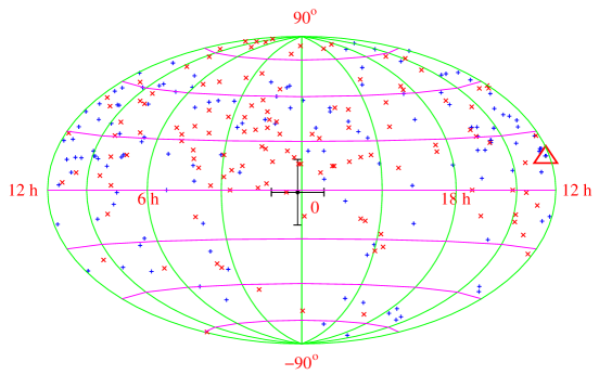
Figure 2: Aithoff-Hammer equal-area plot of $\sin 2\beta$, where $\beta$ is the difference in the polarization position angle and the orientation angle of the source. We represent $\sin 2\beta<0.0$ by blue pluses while $\sin 2\beta\geq 0.0$ is represented by red crosses. The dipole anisotropy axis, $[(0\ h,9\ m)\pm(1\ h,0\ m),-1^{o}\pm 15^{o}]$, obtained by Jain & Ralston (1999) is shown along with its error bars. The position of the Virgo supercluster is shown with a red triangle. The cut $|RM-6|>6$ has been used in this plot.

The above lack of correlation between $RM$ and $\beta$, however, does not rule out the possibility that the value of $\beta$ is randomized due to biased extraction of $RM$. This might happen preferentially in the regions of large magnetic field i.e. where $RM$ is large. As we have discussed earlier, the distribution of $\beta$ peaks at $\pi/2$. If in a certain patch the values of $\beta$ are randomized, then the mean value of $\beta$ in this patch will deviate significantly from $\pi/2$ and could in principle give rise to a large value of the statistic indicating correlation.

We next investigate whether the correlation arises due such a randomization. In Figure 2 we plot the sign of $\sin 2\beta$ over the dome of the sky in the equatorial coordinate system after making the cut $|RM-6|>6$. Here the sources with $\sin 2\beta<0.0$ and $\sin 2\beta\geq 0.0$ are represented by plusses and crosses respectively. From this figure we see that the positive values of $\sin 2\beta$ dominate near the dipole anisotropy axis given in Equation 6. Figure 2 clearly indicates that there indeed exists an anisotropy in the polarizations of radio galaxies and there exist large patches where the value of $\sin{2\beta}$ is either positive or negative. Hence we find no evidence that the correlation seen in data arises due to randomization of $\beta$ in some regions. We may quantize this clustering of negative and positive values of $\sin 2\beta$ by defining a new statistic. We consider a $N_{n}$ number of nearest neighbours of the source $i$. For these $N_{n}$ sources we set $x_{i}=1$ if $\sin 2\beta\geq 0$ and $x_{i}=-1$ if $\sin 2\beta<0$. We then compute $X_{i}=|\sum_{i}x_{i}|$ and the statistic $X$ is obtained by summing $X_{i}$ over the entire data sample. The $P$-value in this case is computed by comparing with a large number of random samples obtained by shuffling the $\beta$ values of the data. The resulting $P$-values or the significance level for the complete data sample and for the set obtained after making the cut $|RM-6|>6$ are shown in Figure 3. We find that $P\approx 0.2-0.5$% for the complete sample and $P\approx 2.5\times 10^{-4}-6.0\times 10^{-4}$% after the cut. In Figure 4 we show the histogram of the statistic $X$ generated using 10000 random data samples. This figure also clearly shows that the statistic of the data sample lies far above the peak value of the histogram. The very small $P$-values obtained after the cut is a clear indication that $\beta$ values in the different regions of the sky are indeed correlated with one another. This is infact another confirmation of the large correlation found by Jain & Ralston (1999). Hence we dismiss the above explanation in terms of bias in the extraction of $IPA$.

An improved statistical procedure for extraction of rotation measures and IPA was proposed by Sarala & Jain (2001, 2002). Using the revised $\beta$ values obtained by this procedure, the Jupp-Mardia test for anisotropy gives $P=0.1$ %. Hence these revised $\beta$ values continue to support the presence of anisotropy in the data.

Figure 3: The $P$-value(%) using the $X$ statistic is plotted as the function of the number of nearest neighbours. The result is shown for both the complete set($332$ points) and with the cut in the $RM$ ($265$ points).

Figure 4: The histogram of $X$ statistic using 10000 random samples obtained by shuffling the $\beta$ values of the data with the cut $|RM-6|>6$. The number of nearest neighbours is taken to be 135 at which the $P$-value is found to be the smallest. The statistic of the data in this case is equal to 0.165, shown by the dotted line, and the corresponding $P=2.5\times 10^{-4}$ %.

Cuts	n	$n\rho^{2}$
Full data	332	1.742
$|RM-6|>6$	265	1.780
$|RM|<100$	278	4.341
$|RM|<70$	254	1.101
$|RM|<100$ and $|RM-6|>6$	211	4.320

Table 1: JM correlation between $RM$ and $\beta$ with different cuts in the $RM$.

In order to further examine the effect of rotation measures on the observed anisotropy we examine how the correlation changes if we eliminate the sources which lie close to the galactic plane. The dominant contribution to $RM$ is obtained from the milky way and hence largest values of $RM$ are observed for these sources. We therefore impose a cut on the data to eliminate sources with the galactic latitude $|b|\leq 30^{o}$. This leaves a total of 214 sources in the data set. We repeat the JM correlation discussed earlier using Map 3. We find that the statistic $n\rho^{2}=9.43$ after the galactic cut and this implies that the anisotropy in $\beta$ persists with about 98% confidence level. As expected, the anisotropy is enhanced by making a cut in the $RM$ such that only the sources which statisfy $|RM-6|>6.0$ are included. The results are tabulated in Table 2. We see from the table that the statistic does not change much in comparison with the data without the galactic cut. Hence we find that the regions of large $RM$ do not necessarily imply large correlation of $\beta$.

	n	$n\rho^{2}$	P (%)
Full Set	214	9.43	2
$|(RM-6|>6.0$	155	22.33	0.04∗

Table 2: The $n\rho^{2}$ values after eliminating sources lying in the galactic plane. Results are given for the full set as well as with a cut in the Rotation Measure. ^∗The $P$ value for the cut $|(RM-6)|>6.0$ is obtained by using $\chi^{2}_{5}$.

The above discussion clearly shows that the correlation seen in the data is not a direct consequence of the correlation of the RM with the angular coordinates of the source. However the cut in RM does result in a large increase in the signal of anisotropy and hence in some sense it must depend on RM. One possibility is that the sources eliminated by the cut show a random behaviour and are uncorrelated. This turns out to be not true. Instead we find that the sources eliminated by the cut show an opposite angular dependence in comparison to the remaining sources. We illustrate this by making the following ansatz for the joint distribution

$$F(\beta,{\bf R})h({\bf R})=\exp\left[k\cos{\Omega}+\mbox{\boldmath$\lambda$}\cdot{\bf R}(1+g(RM))\sin{\Omega}\right]h({\bf R})$$ (7)

where as defined earlier $\Omega=2\beta+\nu\sin 2\beta$ and $g(x)$ is taken to be a gaussian,

$$g(x)=c_{1}\pi\exp\left[-(x-c_{2})^{2}/c_{3}^{2}\right]\ .$$ (8)

Here we have introduced three new parameters $c_{1},c_{2}$ and $c_{3}$. The difference of maximum likelihood between this correlated ansatz and the null ansatz turns out to be 17.6 for the entire data set of 332 sources. Here the null ansatz is the two parameter distribution obtained by using the transformation 5 in the von Mises distribution. This “sharply peaked” distribution can be written as

$$S(\beta)=const\times e^{k\cos(2\beta+\nu\sin 2\beta)}$$ (9)

The statistical significance of the signal of correlation in this case is

$$P=3.8\times 10^{-4}\%\ ,$$

taking into account the eight parameters in the correlation ansatz. If the null hypothesis is assumed to be the von Mises distribution we find an even smaller value of $P$. The signal of correlation is clearly very strong and cannot be dismissed as a statistical fluctuation. The parameters are given by $k=-0.561\pm 0.071$, $\nu=-1.09\pm 0.17$, $c_{1}=-1.71\pm 0.32$, $c_{2}=9.64\pm 0.47$, $c_{3}=2.89\pm 0.55$, $|\mbox{\boldmath$\lambda$}|=0.70\pm 0.15$ and the axis parameters are given by

$$RA=(0^{\rm h},\ 3.7^{\rm m})\pm(0^{\rm h},\ 46^{\rm m}),\ DEC=-10.7^{o}\pm 12.2^{o}$$ (10)

in the B1950 coordinate system. Within errors this points opposite to the direction of the Virgo supercluster. We see from the value of the parameter $c_{1}$ that the sources whose RM lies roughly within the interval $c_{2}\pm c_{3}$ show a correlation with $\mbox{\boldmath$\lambda$}\cdot{\bf R}$ which is opposite to the remaining sources. The correlation term $\mbox{\boldmath$\lambda$}\cdot{\bf R}(1+g(RM))$ has an opposite sign for these sources in comparison to the remaining sources. The axis parameters, Eq. 10, obtained from this fit agree with the earlier fit, Eq. 6, within errors.

The function $g(RM)$ essentially treats the sources whose RM lies in the interval $c_{2}\pm c_{3}$ differently from the remaining sources. This interval is centered at the value $c_{2}$ which is very close to the position of the peak in the RM distribution as can be seen in Fig. 1. We may attribute this shift in the peak to some bias in the extraction of RM or due to some systematic physical effect such as the contribution due to the milky way. Hence if the difference $RM-c_{2}$ is small it may indicate that the host contribution to RM is negligible. The introduction of the function $g(RM)$ in the correlation ansatz, therefore, treats the sources with negligible contribution due to the host galaxy differently than the remaining sources.

The relationship between $\beta$ and the position vector $R$ of the source indicated by Eq. 7 may be expressed as follows,

$${<(1+\nu\cos 2\beta)sin{\Omega}>\over<(1+\nu\cos 2\beta)cos{\Omega}>}={\mbox{\boldmath$\lambda$}\cdot{\bf R}\over k}(1+g(RM))\$$ (11)

where the angular brackets indicate statistical averages. Since the parameter $\nu\approx-1$, the function $(1+\nu\cos 2\beta)$ is approximately 2 near the peak of the distribution of $\beta$ and zero near the tail. Hence this function weights the peak region more than the tail in the statistical averages. For $\beta$ close to its peak value $\pi/2$, we find that $\sin{\Omega}\approx-2(1-\nu)(\beta-\pi/2)$ and $\cos{\Omega}\approx-1$. If $RM$ is not too close to its peak value or more precisely $|RM-c_{2}|>c_{3}$ then $g(RM)\approx 1$ and hence we find the approximate relation

$$<\beta-\pi/2>\approx{1\over 2(1-\nu)}{\mbox{\boldmath$\lambda$}\cdot{\bf R}\over k}\ ,$$ (12)

which is same as the relationship given in Eq. 2 with the $\Lambda$ in Eq. 2 identified with ${\mbox{\boldmath$\lambda$}\over(1-\nu)k}$ in Eq. 12.

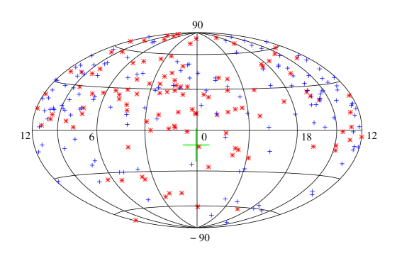
Figure 5: Aithoff-Hammer scatter plot of the correlation variable $(1+g(RM))\sin\Omega$, as defined in Eq. 7. Here red stars and blue plusses represent sources for which $(1+g(RM))\sin\Omega>0.1$ and $(1+g(RM))\sin\Omega<-0.1$ respectively. The anisotropy axis, $[(0^{\rm h},\ 3.70^{\rm m})\pm(0^{\rm h},\ 46^{\rm m}),-10.7^{o}\pm 12.2^{o}]$, along with its error bars is shown in green.

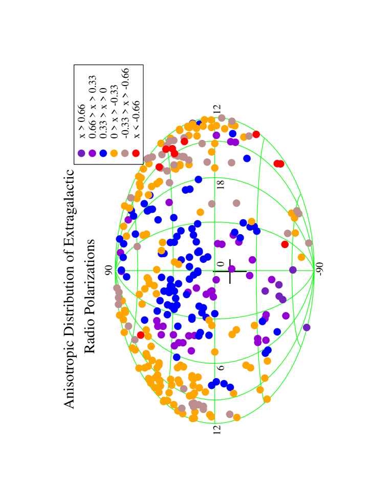
Figure 6: Aithoff-Hammer scatter plot of the averaged correlation variable $x=\overline{(1+g(RM))\sin\Omega}$, as defined in Eq. 7. For each source located in the direction $R_{1}$ we take the average over all the nearest neighbours which lie within the cone defined by $\mbox{\boldmath$R_{1}$}\cdot\mbox{\boldmath$R_{2}$}<0.95$, where $R_{2}$ is the unit vector in the direction of any other source. The anisotropy axis, $[(0^{\rm h},\ 3.70^{\rm m})\pm(0^{\rm h},\ 46^{\rm m}),-10.7^{o}\pm 12.2^{o}]$, is shown along with its error bars. Within errors it points opposite to the Virgo supercluster.

The anisotropic distribution of the offset angle obtained with the fit Eq. 7 may now be illustrated by making an Aithoff-Hammer scatter plot of the correlation variable $(1+g(RM))\sin\Omega$. This is shown in fig. 5 where stars and plusses represent sources for which $(1+g(RM))\sin\Omega>0.1$ and $(1+g(RM))\sin\Omega<0.1$ respectively. We find that the stars are concentrated in the direction of the axis with the plusses concentrated in the opposite direction. The anisotropy in the angular distribution of the offset angles is clear from this plot. The nature of the anisotropy is also nicely illustrated by making a scatter plot after taking the local averages. In fig. 6 we show the Aithoff-Hammer scatter plot of the averaged correlation variable, $\overline{(1+g(RM))\sin\Omega}$, at the location of each source. The average is done over the nearest neighbours whose angular separation from the source is less than $\cos^{-1}0.95\approx 18^{o}$. The mean number of sources which contribute to this average is found to be 12.6. The plot clearly shows anisotropic nature of the distribution of the offset angles.

3. Physical Origin of the Effect

From the results obtained above we see that the offset angle $\beta$ shows some correlation with $RM$ but the correlation is direction dependent. It is difficult to visualize how such a direction dependent correlation can arise due to bias in data. In all likelihood this is caused by some physical phenomenon. The offset angles of the different sources may be intrinsically correlated or the effect may arise due to propagation. The possibility of intrinsic correlation can be further investigated by determining the correlation of the intrinsic position angle of polarization $\chi$ and the orientation angle of the galaxy $\psi$ among the different sources. By using the statistical techniques used in (Hutsemékers 1998, Hutsemékers & Lamy 2001, Jain, Narain & Sarala 2003) to test of alignment of optical polarizations, we find that $\chi$ and $\psi$ for different sources show no alignment with one another. The $P$ value in this case is found to be larger than 10 % independent of the number of nearest neighbours used to test for alignment. Hence it is not possible to attribute the radio anisotropy to intrinsic alignment of radio polarization and it is likely to arise due to some propagation effect. Within conventional physics the corrections to the Faraday polarization rotation effect are very small and hence it is unlikely that this anisotropy may be explained within this framework. The anisotropy may, therefore, be an indication of some new physical effect.

One interesting possibility is the presence of a very low mass background pseudoscalar field in the universe. We assume that at large redshifts, relevant for the sources considered in the present data set, this field has a coherent component which is approximately given as

$$\phi({\bf R})\approx\phi_{0}\cos(\theta)(1+g[B_{r}({\bf R})])$$ (13)

where $\phi_{0}$ is a constant independent of redshift, $\theta$ is the angular position of the source measured with respect to the prefered axis $\lambda$, $B_{r}$ is the radial component of the magnetic field in the coordinate frame with origin located at the observation point i.e. earth and $g(B_{r})$ is a gaussian defined in Eq. 8. At the position of the earth we assume that this field acquires a value $\phi_{1}$. The total rotation in the polarization angle due to this field is then equal to $\phi(\bf R)-\phi_{1}$ (Harari & Sikivie, 1992). Since the rotation measure is proportional to $B_{r}$ we find that this effect can explain the observed correlation given in Eq. 7. This mechanism requires a large scale anisotropy in the universe and provides the simplest explanation of the observations.

We next determine whether the observations can also be explained within the framework of an isotropic universe. Although the correlation indicates the presence of a global anisotropy it is possible that the correlation may arise due to the existence of a few patches of length scales of order Gpc over which the pseudoscalar field shows a coherent dependence as a function of the angular coordinates. For example there may exist two such patches, one in the direction of the axis and another in the opposite direction. The observed anisotropy can arise if the pseudoscalar field in one of these patches is approximately equal to the negative of its value in the other patch. In particular the observed correlation can be explained if $\phi({\bf R})\approx\phi_{0}(1+g(RM))$ in one of the patches and $\phi({\bf R})\approx-\phi_{0}(1+g(RM))$ in the second patch. We point out that although the existence of a large scale dipole distribution of the background field violates the fundamental assumption of isotropy of the universe, the existence of the few patches of length scales of order Gpc does not. Here we also assume that in eq. 13 $\phi({\bf R})$ depends on the magnitude $|{\bf B}|$ rather than on $B_{r}$. Such a functional dependence may also explain the observations provided we attribute the RM contribution due to the host galaxy to the deviation of RM from its peak value, RM_peak, in the RM distribution. As discussed earlier, our fits also always select the parameter $c_{2}$ such that it is approximately equal to RM_peak. The shift in RM_peak from zero may be attributed to some local effect such as the contribution due to the milky way or due to some bias in the extraction of RM. The deviation of RM from its peak value, RM-RM_peak, gets contribution both from the host galaxy and the milky way. Hence RM-RM_peak is directly proportional to the magnitude of the magnetic field in the host galaxy, assuming that in a statistical sense all the components of the background magnetic field have equal strength. This mechanism may explain the observed correlation within the framework of an isotropic universe provided their exist patches of coherent background pseudoscalar field of length scales of order Gpc. However coherence on such large scales is not expected in conventional cosmology. Furthermore this explanation also requires an accidental correlation of two oppositely directed patches such that pseudoscalar field is positive in one of these patches and negative in the other.

A large scale anisotropy has also been observed in the optical polarizations from distant quasars (Hutsemékers 1998, Hutsemékers & Lamy 2001, Jain et al. 2003). It was found that the optical polarizations are aligned with one another over very large distances of the order of Gpc. A very strong alignment was seen in a patch at large redshifts centered at the Virgo supercluster (Hutsemékers 1998). Furthermore it was found (Jain et al 2003) that the polarizations of the large redshift, $z\geq 1$, data sample are aligned over the entire celestial sphere. This effect is also not easily explained within conventional cosmology/astrophysics. The effect may have some relationship to the radio anisotropy discussed in this paper since both the effects appear to be very strong in the direction of the Virgo supercluster. As shown in Jain et al. (2003) the optical alignment effect can also be explained if we assume the existence of a light pseudoscalar. The proposed explanation requires the existence of several patches of large scale magnetic fields of length scales of order Gpc. Furthermore the global alignment at large redshifts requires the existence of a magnetic field coherent over the entire universe. Alternatively this very large scale alignment can be explained if the large redshift QSO’s emit a significant flux of light pseudoscalars at optical frequencies.

4. Conclusions

To conclude, we find that there is considerable evidence for the presence of angular correlation in the radio offset angles which is not easily explained within conventional cosmology/astrophysics. The effect may be explained by the presence of a hypothetical pseudoscalar particle. The effect indicates the existence of a global anisotropy in the universe.

Acknowledgements: We thank Amir Hajian and John Ralston for useful comments.

References

• Bietenholz M. F., Kronberg P. P., 1984, ApJ, 287, L1-L2

• Birch P., 1982, Nature, 298, 451

• Broten N. W., MacLeod J. M., Vallee J. P., 1988, Astrophysics and Space Science 141, 303

• Dobado A., Maroto A. L., 1997, astro-ph/9706044, Mod. Phys. Lett. A 12, 3003

• Harari D., Sikivie P., 1992, Phys. Lett. B 289, 67

• Hutsemékers D., 1998, A & A 332, 410

• Hutsemékers D., Lamy H., 2001, A & A, 367, 381

• Jain P., Ralston J. P., 1999, Mod. Phys. Lett. A14, 417

• Jain P., Panda S., Sarala S., 2002, Phys. Rev. D 66, 085007; hep-ph/0206046

• Jain P., Narain G., Sarala S., 2003, astro-ph/0301530, to be published in MNRAS

• Jupp P. E., Mardia K. V., 1980, Biometrika 67, 163

• Kendall D. G., Young A. G., 1984, MNRAS, 207, 637

• Mansouri R., Nozari K., 1997, gr-qc/9710028

• Moffat J. W., 1997, astro-ph/9704300

• Obukhov Y. N., 2000, astro-ph/0008106, Published in Colloquium on Cosmic Rotation: Proceedings edited by M. Scherfner, T. Chrobok and M. Shefaat (Wissenschaft und Technik Verlag: Berlin, 2000), 23-96.

• Obukhov Y. N., Korotky V. A., Hehl F. W., 1997, astro-ph/9705243

• Phinney E. S., Webster R. I., 1983, Nature 301, 735

• Ralston J. P., Jain P., 1999, International Journal of Modern Physics D 8, 537

• Sarala S., Jain P., 2001, astro-ph/0007251, MNRAS 328, 623

• Sarala S., Jain P., 2002, Journal of Astrophysics and Astronomy 23, 137

• Surpi G. C., Harari D. D., 1999, astro-ph/9709087, ApJ 515, 455

• Vallée J. P., 1997, Fundamentals of Cosmic Physics 19, 1

• Zeldovich Ya. B., Ruzmaikin A. A., Sokoloff D. D., 1983, Magnetic fields in Astrophysics (Gordon and Breach Science Publishers, 1983).