Ultraviolet Line Emission from Metals in the Low-Redshift Intergalactic Medium

Abstract

We use a high-resolution cosmological simulation that includes hydrodynamics, multiphase star formation, and galactic winds to predict the distribution of metal line emission at $z\sim 0$ from the intergalactic medium (IGM). We focus on two ultraviolet doublet transitions, O VI $\lambda\lambda 1032,1038$ and C IV $\lambda\lambda 1548,1551$. Emission from filaments with moderate overdensities is orders of magnitude smaller than the background, but isolated emission from enriched, dense regions with $T\sim 10^{5}$–$10^{5.5}\mbox{ K}$ and characteristic size $\sim 50$–$100\mbox{ kpc}$ can be detected above the background. We show that the emission from these regions is substantially greater when we use the metallicities predicted by the simulation (which includes enrichment through galactic winds) than when we assume a uniform IGM metallicity. Luminous regions correspond to volumes that have recently been influenced by galactic winds. We also show that the line emission is clustered on scales $\sim 1h^{-1}\mbox{ Mpc}$. We argue that although these transitions are not effective tracers of the warm-hot intergalactic medium, they do provide a route to study the chemical enrichment of the IGM and the physics of galactic winds.

1. Introduction

The modern paradigm for cosmological structure formation, the cold dark matter model, has had admirable success in describing both the formation of galaxies and the distribution of matter on larger scales. The model predicts that small perturbations in the early universe grow through gravitational instability and eventually collapse to form the objects we see around us. As collapse proceeds, matter collects in a “cosmic web” of mildly overdense sheets and filaments, with galaxies and galaxy clusters at their intersection. Simulations and analytic studies have shown that these gas structures are responsible for the so-called Ly$\alpha$ forest of absorption lines in quasar spectra (e.g., Bi et al. 1992; Bi 1993; Cen et al. 1994; Zhang et al. 1995; Hernquist et al. 1996; Theuns et al. 1998; Davé et al. 1999). However, as observations and simulations have improved, it has become clear that the intergalactic medium (IGM) has experienced a variety of complex processes, including shock heating and feedback from galaxies.

Most important, it now appears that a substantial fraction of the originally pristine intergalactic gas was enriched with a small, but significant, amount of heavy elements through interactions with star-forming galaxies. The best evidence for enrichment comes from detailed spectroscopic studies of the high-redshift Ly$\alpha$ forest. Matching individual Ly$\alpha$ absorption features with absorption in the corresponding wavelength range for metal transitions (especially the C IV $\lambda\lambda 1548,1551$ and O VI $\lambda\lambda 1032,1038$ doublets) has revealed that high-column density absorbers (with $N_{\rm HI}\gtrsim 10^{14.5}\mbox{ cm${}^{-2}$}$, corresponding to physical overdensities of a few; e.g., Schaye 2001) are almost universally enriched to $Z\gtrsim 10^{-3}Z_{\sun}$ (Tytler et al., 1995; Cowie et al., 1995; Songaila & Cowie, 1996; Davé et al., 1998; Carswell et al., 2002). Pixel-by-pixel analyses have revealed the presence of metals in even lower column density absorbers (Cowie & Songaila, 1998; Ellison et al., 2000; Schaye et al., 2000, 2003; Aracil et al., 2003; Pieri & Haehnelt, 2003), although the scatter in the metallicity is large and there is evidence for a decrease in metallicity with decreasing overdensity (Schaye et al., 2003). Metals therefore appear to be widespread in the IGM, although the mechanism through which they were dispersed remains to be determined.

The leading candidate is expulsion from star-forming galaxies through winds driven by supernovae, possibly aided by radiation pressure (e.g. Aguirre et al. 2001a). Such winds have been observed both in nearby starburst galaxies (e.g., Lehnert & Heckman 1996; Heckman et al. 2000; Martin 1999) and in star-forming Lyman-break galaxies at $z\sim 3$ (Pettini et al., 2001, 2002; Shapley et al., 2003), but their power, duration, and filling factor remain unclear. There is also a theoretical expectation that similar winds may have occurred in high-redshift dwarf galaxies, because the small binding energies of these systems would allow a wind to escape fairly easily (Dekel & Silk, 1986; Madau et al., 2001; Bromm et al., 2003; Furlanetto & Loeb, 2003). The time history of enrichment has important implications not only for the characteristics of the present-day IGM but also for such topics as the reionization history of the universe (Wyithe & Loeb, 2003a, b; Cen, 2003; Sokasian et al., 2003) and ending the era of Population III star formation (Bromm et al., 2001; Oh et al., 2001; Mackey et al., 2003). Detailed studies of the distribution of metals in the IGM will help to determine how and when enrichment occurred. Careful analysis of Ly$\alpha$ forest absorption spectra is one promising approach. However, absorption studies of the Ly$\alpha$ forest can only provide information along isolated lines of sight to quasars, giving no more than an indirect picture of metals in the IGM. It would thus be useful to find some technique to directly trace the distribution of metals in three dimensions.

One such method is to search for metal line emission from the IGM. Because emission does not rely on the existence of a background source, it can be imaged over large fields of view. With the addition of individual line redshifts, we can construct a three-dimensional picture of the metal distribution (in a similar way to galaxy redshift surveys). Observations in this direction have begun: diffuse O VI $\lambda 1032$ emission has been detected from our own Galaxy (Shelton et al., 2001; Dixon et al., 2001; Welsh et al., 2002) and above the disks of edge-on spirals (Otte et al., 2003), while Hoopes et al. (2003) place limits on the emission from galactic winds. Because of the complexity of the emission processes, and their sensitive dependence on temperature and density, this question is best addressed through detailed cosmological simulations. In this paper, we use such a simulation to calculate emission from the IGM in the two ultraviolet (UV) doublets O VI $\lambda\lambda 1032,1038$ and C IV $\lambda\lambda 1548,1551$. We note that doublets are particularly useful because they allow an unambiguous identification of the line feature. We focus on emission from the low-redshift ($z\lesssim 0.25$) universe that is most likely to be observable in the near future. We will contrast a uniform metallicity with the metal distribution predicted by the simulation, which includes winds from massive galaxies.

Aside from enrichment, another key process affecting IGM gas is shock heating: simulations show that a large fraction ($\gtrsim 20\%$) of intergalactic gas has $10^{5}\mbox{ K}\lesssim T\lesssim 10^{7}\mbox{ K}$ (Cen & Ostriker, 1999; Davé et al., 2001). This so-called warm-hot intergalactic medium (or WHIM) is heated through accretion shocks as sheets and filaments assemble into larger structures. WHIM gas does not form a single, well-defined phase: because the shocks are not uniform, it has a wide range of densities, from near the cosmic mean to that characteristic of galaxy groups. But all WHIM gas shares one crucial characteristic: because it is too warm to form stars but too cool to produce X-rays, it is very difficult to detect. The difficulty is severe enough that gas at or near the cosmic mean density, whose surface brightness is particularly small, is referred to as the “missing baryons.” One technique to search for WHIM gas is to use absorption systems (Perna & Loeb, 1998; Hellsten et al., 1998). Tripp et al. (2000) found a large number of low-redshift O VI $\lambda 1032$ absorbers along one line of sight, suggesting that $\gtrsim 10\%$ of baryons are in the WHIM phase. However, these absorption studies suffer from the same drawbacks mentioned above and do not provide a direct picture of WHIM gas. Images of its distribution could thus test predictions about the gravitational growth of structure. Simulations have shown that transitions of higher ionization stages of oxygen (O VII and O VIII) are effective probes of the higher-temperature part of WHIM gas (Yoshikawa et al., 2003). We will investigate whether emission from the O VI $\lambda 1032$ and C IV $\lambda 1548$ transitions will allow one to map the distribution of the lower-temperature portion of the WHIM gas. Because gas in the appropriate temperature range is expected to lie in sheets and filaments, this technique would offer the additional advantage of tracing the cosmic web, providing further confirmation of the cold dark matter paradigm.

We first calculate the line emissivity of a given gas parcel in §2. We then describe our simulation and show how to calculate the emission from it in §3. We discuss our results in §4 and conclude in §5.

2. Metal Emission Mechanisms

We consider the emission from two metal line doublets: O VI $\lambda\lambda 1032,1038$ and C IV $\lambda\lambda 1548,1551$. For each doublet, we use Cloudy 94 (Ferland, 2000, 2001) to compute the emissivity of a given parcel of gas. We first construct a grid of densities and temperatures spanning the entire range of particle properties in our simulation. We choose density spacings of $\Delta\log(n_{\rm H}/{\rm cm}^{-3})=0.25$ for $10^{-6}\leq(n_{\rm H}/{\rm cm}^{-3})\leq 10^{-2}$ and $\Delta\log(n_{\rm H}/{\rm cm}^{-3})=1.0$ otherwise. Here $n_{\rm H}$ is the total density of neutral and ionized hydrogen. Because the ionization fractions (and emissivities) are sensitive to variations in the temperature, we choose $\Delta\log(T/{\rm K})=0.05$ for $10^{4.25}\mbox{ K}\leq T\leq 10^{7}\mbox{ K}$ and $\Delta\log(T/{\rm K})=0.25$ elsewhere. We then generate grids of the emissivity for each transition, including collisional or radiative excitation followed by radiative de-excitation as well as recombination cascades. However, photon emission following absorption of a photon of the same wavelength does not contribute to the net emission. We therefore use Cloudy to compute this “pumping” component separately and subtract it from the total emissivity. We generate the grids at solar metallicity; the emissivity is proportional to the metallicity. For each of these transitions, the shorter wavelength line is also the stronger member of the doublet, with a flux ratio of 2:1. For concreteness, we quote results for the stronger line in the following.

Table 1Ionizing Background Models

Name	$\log(\Gamma_{\rm HI}/{\rm s}^{-1})$	$\Phi_{1026}$	$\Phi_{1216}$	$\Phi_{1551}$	$\Phi_{1815}$
HM01	-13.1	29.3	81.7	154	182
HM01s	-12.5	111	309	582	688
HM01w	-14.0	3.5	9.8	18.4	21.8
HM96	-13.1	4.1	5.0	6.5	7.0
Coll	–	–	–	–	–

Note. — Models labeled ‘HM96’ and ‘HM01’ use the spectral shapes of Haardt & Madau (1996) and Haardt & Madau (2001), respectively. Model ‘Coll’ assumes pure collisional ionization. All surface brightness values are reported in photons cm^-2 s^-1 sr^-1 Å^-1.

Because most of the IGM is photoionized, our choice of ionizing background could significantly affect the results. Unfortunately the ionizing background at $z\sim 0$ is relatively poorly constrained. Davé & Tripp (2001) use observations of the low-redshift Ly$\alpha$ forest to estimate a total H I ionizing rate of $\Gamma_{\rm HI}=10^{-13.3\pm 0.7}\mbox{ s${}^{-1}$}$ at $z=0.17$. The shape of the spectrum is even more poorly known, because the extragalactic background is difficult to measure directly at these wavelengths, particularly blueward of Ly$\alpha$. Brown et al. (2000) estimate a surface brightness of $\Phi(1450$–$1900\mbox{ \AA})\sim 500\pm 100\mbox{ photons cm${}^{-2}$ s${}^{-1}$ sr${}^{-1}$ \AA${}^{-1}$}$ based on Hubble Space Telescope observations of diffuse radiation along a low-extinction line of sight through the Galaxy. The best limits in the range 912–1216 Å come from the Voyager spacecraft; Murthy et al. (1999) place a $1\sigma$ upper limit of $\Phi(912$–$1216\mbox{ \AA})<30\mbox{ photons cm${}^{-2}$ s${}^{-1}$ sr${}^{-1}$ \AA${}^{-1}$}$, although Edelstein et al. (2000) argue that systematic uncertainties increase the limit to $\Phi(912$–$1216\mbox{ \AA})<10^{4}\mbox{ photons cm${}^{-2}$ s${}^{-1}$ sr${}^{-1}$ \AA${}^{-1}$}$ at the $2\sigma$ level.

Figure 1.— The normalized emissivity $\varepsilon/n_{\rm H}^{2}$ of O VI $\lambda 1032$ . All the panels except the bottom right show contour plots in the $n_{\rm H}$–$T$ plane assuming different ionizing backgrounds (see text for details). Upper left: HM01. Upper right: HM96. Lower left: HM01w. Lower right: The emissivity assuming collisional equilibrium (solid curve). Note that this quantity is independent of density. We also show $\varepsilon/n_{\rm H}^{2}$ for the HM01 spectrum assuming $n_{\rm H}=10^{-6},\,10^{-4}$, and $10^{-2}\mbox{ cm${}^{-3}$}$ (dotted, dashed, and dot-dashed curves, respectively).

Because of this uncertainty, we include several choices for the radiation background. We base our models on the spectra presented in Haardt & Madau (1996,  hereafter HM96), which includes only the contribution of quasars, and Haardt & Madau (2001,  hereafter HM01), which includes both quasars and star-forming galaxies. We vary the normalizations of these spectra over the range allowed by Davé & Tripp (2001). We also include a model assuming pure collisional ionization and excitation. We summarize the characteristics of our ionizing backgrounds in Table 1, including the total ionizing rate and estimates of the background levels at each of several wavelengths. Comparing these results to the direct measurements described in the previous paragraph, the HM01 model appears to provide a reasonable fit to the data, although it does underestimate the flux redward of Ly$\alpha$ reported by Brown et al. (2000). Note that, even with $\Gamma_{\rm HI}$ fixed, the HM96 model background is much smaller than that of the HM01 model at the listed wavelengths. This is simply because galaxies dominate the background redward of the Lyman limit, while quasars dominate blueward of this limit. Because it does not include galaxies, the HM96 model strongly underestimates the background at $\sim 1000$–$2000$ Å.

The resulting emissivity grids are shown in Figure 1 for O VI $\lambda 1032$ and Figure 2 for C IV $\lambda 1548$. We display, using logarithmic contours, the density-normalized line emissivity $\varepsilon/n_{\rm H}^{2}$ (in units of erg cm³ s^-1). In such units, the emissivity in a purely collisionally ionized gas is independent of density. Three of the panels show contour plots of the emissivity for different choices of the ionizing spectrum: HM01 (top left), HM96 (top right), and HM01w (bottom left). We draw contours at intervals of $\Delta\log(\varepsilon/n_{\rm H}^{2})=1.0$ and label the highest contour in each panel for clarity. The bottom right panel in each figure shows a line plot of $\varepsilon/n_{\rm H}^{2}$ as a function of temperature. The solid line assumes pure collisional ionization, while the dotted, dashed and dot-dashed curves assume the HM01 background with $n_{\rm H}=10^{-6},\,10^{-4}$, and $10^{-2}\mbox{ cm${}^{-3}$}$, respectively. We see that O VI $\lambda 1032$ efficiently probes gas with $T\sim 10^{5.5}\mbox{ K}$, while C IV $\lambda 1548$ probes gas with $T\sim 10^{5}\mbox{ K}$. Note that the line emissivities are quite sensitive to the temperature, and a realistic prediction of the IGM emission requires an accurate treatment of heating and cooling processes. The bottom right panels show that photoionization has a substantial effect on the emissivity of the low-density IGM: it increases the emission from cool gas but decreases the emission from hot gas. The photoionizing background drives low-density gas to higher ionization states than it would otherwise assume. On the other hand, these panels also show that the photoionizing flux makes little difference for gas with $n_{\rm H}/\bar{n}_{\rm H}\gtrsim 100$. Such gas is dense enough for collisional processes to dominate over any reasonable ionizing background. A comparison of the HM01 and HM01w panels shows that, for lower densities, the emissivity quickly returns to the collisional ionization values as the ionizing photon flux decreases (because the number of available ionizing photons decreases, so the maximum gas density that can be affected declines). Finally, note that the HM96 and HM01 spectra yield nearly identical results, despite the large differences in the background fluxes for $\lambda\sim 1000$–$2000$ Å. This is because we have removed the pumping contribution to the emissivity and because the ionization potentials for these species are high, well into the regime in which quasars dominate the spectrum.

Figure 2.— Same as Figure 1, but for C IV $\lambda 1548$.

One uncertainty in our emissivity calculations is that they implicitly assume ionization equilibrium. Testing this assumption precisely is difficult because equilibrium for high-ionization state metals depends on a large number of separate recombinations. However, it appears to be a reasonable assumption. We have used Cloudy to compute the recombination (and collisional ionization) times of C IV and O VI, along with those of the neighboring ionization states, in the range $4.75<\log(T/{\rm K})<6.0$. For metallicities $Z\lesssim 0.1Z_{\sun}$, the recombination and ionization timescales are generally smaller than the cooling timescale by a factor of a few. For significantly higher metallicities, the times become comparable. In this case, the emissivity of gas near the excitation temperature of a given transition will decrease (because the relevant ionization state would be less abundant than expected in equilibrium). However, the gas will emit over a wider temperature regime – and hence for a longer time – as it passes through the O VI and C IV states. The net effect will be to make the emissivity somewhat less sensitive to the gas temperature, but only in the highest metallicity regions.

We also consider two hydrogen lines that may be sources of background contamination in metal line studies: Ly$\alpha$ $\lambda 1216$ (which may be confused with C IV $\lambda 1548$ emitted from lower redshifts) and Ly$\beta$ $\lambda 1026$ (which may be confused with O VI $\lambda 1032$). If an instrument can resolve the O VI or C IV doublets, these lines may be unambiguously identified. Otherwise, single spectral lines like the Lyman series will mimic metal emission. We calculate the total emission in both Ly$\alpha$ and Ly$\beta$ using Cloudy, with the same grid spacings as above. Subtracting the pumping contribution is complicated by the fact that excitations from absorbed background photons do not necessarily produce a Ly$\beta$ photon: the excited state can instead decay to $n=2$ and then to the ground state. (For example, a Ly$\beta$ photon can be “converted” into Ly$\alpha$ and H$\alpha$ photons.) In this case the number of photons removed from the background radiation field by Ly$\beta$ does not necessarily equal the number emitted. We compute the amount of absorption through

$$\varepsilon_{\rm pump}=2\pi n_{\rm HI}\hbar\nu B_{12}\bar{J},$$ (1)

where $n_{\rm HI}$ is the neutral hydrogen density, $B_{12}$ is the Einstein absorption coefficient, $\nu$ is the frequency of the line, and $\bar{J}$ is the background flux averaged over the line profile. For a reasonably smooth background spectrum, $\bar{J}$ is simply equal to the background flux evaluated at the line center. We subtract the amount of energy absorbed from the total emissivity to compute the net emissivity. Note that the net result can be negative if photon conversion dominates over collisional excitation and recombination; in this case we set the emissivity to zero. We compute and subtract the pumping contribution to Ly$\alpha$ using Cloudy, just as for the metal transitions. We refer the reader to Furlanetto et al. (2003) for more information on Ly$\alpha$ emission.

3. The Cosmological Simulation

3.1. Simulation Parameters

We perform all of our calculations within the G5 cosmological simulation of Springel & Hernquist (2003b). This smoothed-particle hydrodynamics (SPH) simulation uses a modified version of the GADGET code (Springel et al., 2001b) incorporating a new conservative formulation of SPH with the specific entropy as an independent variable (Springel & Hernquist, 2002). This “conservative entropy” approach has several advantages over conventional treatments of SPH. Since the energy equation is written with the entropy as the independent thermodynamic variable, the ’$pdV$’ term is not evaluated explicitly, reducing noise. Including terms involving derivatives of the density with respect to the particle smoothing lengths enables this approach to conserve entropy (in regions without shocks), even when smoothing lengths evolve adaptively, avoiding the problems noted by, e.g., Hernquist (1993), and moderates the overcooling problem present in earlier formulations of SPH.

The simulation assumes a $\Lambda$CDM cosmology with $\Omega_{m}=0.3$, $\Omega_{\Lambda}=0.7$, $\Omega_{b}=0.04$, $H_{0}=100h\mbox{ km s${}^{-1}$ Mpc${}^{-1}$}$ (with $h=0.7$), and a scale-invariant primordial power spectrum with index $n=1$ normalized to $\sigma_{8}=0.9$ at the present day. These parameters are consistent with the most recent cosmological observations (e.g., Spergel et al. 2003). The particular simulation we choose has $324^{3}$ dark matter particles and (initially) $324^{3}$ SPH particles in a box with sides of $100h^{-1}$ comoving Mpc, yielding particle masses of $2.12\times 10^{9}h^{-1}\mbox{ M${}_{\odot}$}$ and $3.26\times 10^{8}h^{-1}\mbox{ M${}_{\odot}$}$ for the dark matter and gas components, respectively. The spatial resolution is $8h^{-1}\mbox{ kpc}$ (comoving).

Figures 1 and 2 demonstrate that the emission characteristics of the IGM are extremely sensitive to its temperature and density. We show in Figure 3 the distribution of simulation particles (at $z=0$) in the $n_{\rm H}$–$T$ plane. Note that the colorscale is logarithmic. The phase diagram shows several distinct loci of points. The majority of particles lies along a narrow line connecting underdense, cool gas to moderately overdense, warm gas. This curve represents the unshocked IGM gas, and its shape is fixed by a combination of photoheating and adiabatic expansion (Katz et al., 1996; Hui & Gnedin, 1997; Schaye et al., 1999; McDonald et al., 2001). The second set of particles occupies a much broader range in temperatures at moderate to high overdensities. It represents shocked gas in filaments or virialized halos, including the WHIM gas. A third set of particles lies along a nearly vertical line at $T\sim 10^{4}\mbox{ K}$, representing gas that has cooled and collapsed into bound objects. The rapid decrease in the cooling rate at $T<10^{4}\mbox{ K}$ forces such gas to approach a constant asymptotic temperature slightly below that value. Finally, a fourth set of particles lies at high densities ($n_{\rm H}\gtrsim 0.1\mbox{ cm${}^{-3}$}$) and includes all particles able to form stars.

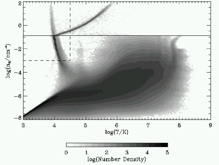
Figure 3.— Phase diagram of simulation particles in the box at $z=0$. The colorscale represents the relative particle density (in logarithmic units). The horizontal solid line marks the threshold density for star formation; we exclude all particles above this line from our analysis. Similarly, the dashed box marks particles expected to be associated with self-shielded regions (also excluded from our analysis).

The simulation includes a new method to describe star formation and feedback in the interstellar medium (ISM) of galaxies (Springel & Hernquist, 2003a). The model divides the ISM into a cold, star-forming component and a low density component heated by supernovae (stars are also included separately). Gas can move between the phases through three processes: star formation, the evaporation of clouds by supernovae, and cooling of the hot phase. This model yields a clearly defined density threshold for star formation ($n_{\rm H}>0.129\mbox{ cm${}^{-3}$}$). Most important, it yields a converged numerical prediction for the cosmic star formation rate within the extended series of simulations performed by Springel & Hernquist (2003b). In fact, using simple physical arguments, Hernquist & Springel (2003) have shown that the evolution of the star formation rate density in these simulations has a simple analytic form that is determined by the gravitational growth of halos (the limiting factor at high redshifts, when cooling times are short) and the expansion rate of the universe (the limiting factor at low redshifts, when cooling times are long). We refer the interested reader to Hernquist & Springel (2003) for more details on the mechanisms driving the star formation history. The suite of simulations performed by Springel & Hernquist (2003b) together with the converged star formation prediction give us confidence that total star formation rates in the simulation we have chosen are unaffected by resolution during the era we study ($z<0.5$).

The star formation model determines the location of star-forming particles in Figure 3. We show the threshold density for star formation by a horizontal solid line. For particles above this threshold, the simulation reports the average temperature of the cold and hot phases. Dense, actively star-forming gas populates the narrow locus of particles with mean temperatures reaching $\sim 10^{6}\,{\rm K}$, while the faint vertical strip at $10^{4}\,{\rm K}$ marks particles that have just been selected by the phenomenological wind model to be ejected from the star-forming phase (see below). Using the method described in Springel & Hernquist (2003a), we could in principle separate the cold (star-forming) gas and the hot (supernova-heated) gas in order to predict the metal line emission from each phase. This would be appropriate if we wished to compute the emission from galaxies themselves. However, such a treatment would ignore the inevitable uncertainties in the local ionizing radiation field (which would be much greater than our assumed diffuse background), dust content, and the geometry of the two phases within each galaxy. Given that the simulation ignores all of these processes, we chose to simply eliminate all star-forming particles from our analysis. As a consequence, our results should be interpreted as excluding emission from galaxies. Galaxies will actually emit strongly in the lines we study (at least relative to pixels without galaxies), but they provide little information about the IGM and can be ignored for the purposes of this investigation.

We also exclude self-shielded gas from our analysis: by definition, the ionizing radiation field in such regions is much smaller than the mean field. We would therefore overestimate the effects of photoionization in such regions. Both simulations (Katz et al., 1996) and analytic estimates (Schaye, 2001) show that self-shielding will only become important in dense, cool regions. We therefore exclude all gas with $n_{\rm H}>10^{-3}\mbox{ cm${}^{-3}$}$ and $T<10^{4.5}\mbox{ K}$ from our analysis. This density threshold marks the point at which the neutral hydrogen column density $N_{\rm HI}\sim 10^{17}\mbox{ cm${}^{-2}$}$ (e.g., Schaye 2001), corresponding to an optical depth to ionizing radiation of unity. These criteria are shown by the dashed lines in Figure 3; we see that self-shielding is only important for gas on or near the cooling locus described above. A comparison with Figures 1 and 2 show that excluding self-shielded gas has only a small effect for C IV $\lambda 1548$ and O VI $\lambda 1032$: the emissivity of gas below this temperature threshold is so small that our results are robust to uncertainties in self-shielding. However, gas in this region of phase space will produce copious numbers of Ly$\alpha$ photons. Our results in this paper therefore underestimate the number of bright Ly$\alpha$ emitting regions; Furlanetto et al. (2003) consider Ly$\alpha$ emission in much more detail.

Note that we do include particles that do not actively form stars but nevertheless lie near galaxies. Of course, local sources of ionizing radiation will also affect such particles. However, because bright particles are primarily collisionally ionized (see §4.6), we do not consider this approximation a bad one. Figure 1 shows that photoionization becomes important when the local ionizing radiation field exceeds the diffuse background by a factor $\sim 100$. This condition will only be satisfied near galaxies; including local ionizing sources will probably increase the signal because much of the gas near galaxies is cooler than the excitation temperature of these transitions. A more serious concern is dust: because many of these particles have recently been ejected from galaxies, they may have significant amounts of dust that redistributes flux emitted through metal lines. We do not attempt to model this process because of the uncertainties involved.

The simulation also includes a model for galactic winds. Such winds are the most plausible mechanism for carrying metals from the star-forming regions in which they are created to the low-density IGM in which they have now been securely detected (e.g., Ellison et al. 2000; Schaye et al. 2003). The volume over which these winds penetrate is clearly critical for understanding the distribution of metals (and hence the distribution of O VI $\lambda 1032$ and C IV $\lambda 1548$ emission), so we review the wind model here (see Springel & Hernquist 2003a for more details). Because of the complexity of the wind generation mechanism in individual galaxies, the treatment must necessarily be phenomenological. We first assume that the disk mass-loss rate in the wind, $\dot{M}_{w}$, is proportional to the star formation rate: $\dot{M}_{w}=\eta\dot{M}_{\star}$. Following the observations of Martin (1999), we set $\eta=2$. We further assume that essentially all of the available supernova energy powers the wind. These conditions fix the wind’s initial velocity at $v_{w}=484\mbox{ km s${}^{-1}$}$. Each particle in a star-forming region is assigned a probability based on $\dot{M}_{w}$ of escaping from the galaxy, and those particles that escape are given a velocity boost in a random direction in such a way that momentum is statistically conserved. Particles that have recently been selected for ejection appear as a high-density “tail” to the cooling IGM gas in Figure 3. It is worth noting that we exclude emission from these particles, although in reality they will contain some enriched, warm gas that may produce metal line emission. However, these particles are directly associated with galaxies and would be difficult to distinguish from their host galaxies.

Note that the simulation itself included a diffuse ionizing background with the shape of HM96, normalized as described in Davé et al. (1999) to match Ly$\alpha$ forest observations. This choice leads to reionization at $z\simeq 6$ and (after this time) largely determines the temperature distribution of the diffuse gas. We therefore cannot include the different heating effects of the ionizing backgrounds described in Table 1; fortunately this will have only a small effect on the observable results. A much more important uncertainty is the cooling function used in the simulations, which does not include metal line emission. To estimate the importance of this effect, we used Cloudy to compare the cooling times (including metal lines) of gas in the range $5<\log(T/{\rm K})<6$ for several different metallicities. We find that for $Z=0.1Z_{\sun}$, the metal lines do have a substantial effect on the cooling times, decreasing them by a factor of $2$–$4$ over metal-free gas. However, the cooling times fall by only $10$–$30\%$ for $Z=0.01Z_{\sun}$. Because the latter value is closer to the mean metallicity in the simulation, we do not expect metal line cooling to have a significant effect in most of the IGM. However, it will affect the characteristics of highly enriched gas, such as that in winds. We would therefore expect winds to cool more quickly through the temperature regime in which they emit strongly, decreasing the number density of such sources by a factor of a few. At the same time, each individual source would be somewhat more compact and hence brighter when it passed through the relevant temperature range. However, we expect the real effect of metal line cooling to be somewhat smaller than this estimate for two reasons. First, increasing the cooling rates will also increase the amount of gas able to form stars, which will in turn increase the amount of energy put into winds. Second, the above cooling time estimate does not include cooling due to the expansion of the wind. In semi-analytic models of winds (e.g. Madau et al. 2001; Furlanetto & Loeb 2003), this cooling mechanism is quite important, so the actual difference between the cooling times will be smaller than suggested above.

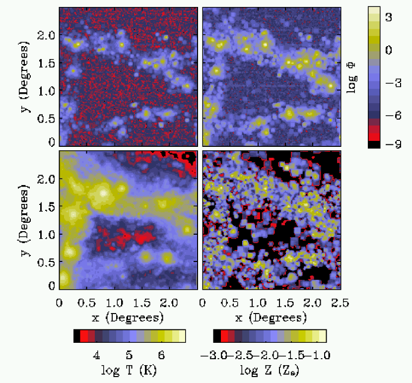
Figure 4.— Maps of a $2.5\arcdeg\times 2.5\arcdeg$ slice of the universe with $z=0.07$, $\Delta z=0.01$, and $\Delta\theta=1\arcmin$. The top row shows the surface brightness of the C IV $\lambda 1548$ (upper left) and O VI $\lambda 1032$ (upper right) transitions assuming simulation metallicities. The colorscale is labeled in units of photons cm^-2 s^-1 sr^-1. The bottom row shows the projected mass-averaged temperature (lower left) and metallicity (lower right).

3.2. Processing the Simulation

Given the emissivity grids and the simulation outputs, we now describe how to calculate the metal line emission from a slice of the universe at redshift $z$ with a specified depth $\Delta z$ and angular width $\theta_{s}$. We first identify the simulation output (or outputs) containing this slice. (Note that the outputs are spaced one light-crossing time apart, so interpolation between them is negligible; see Springel et al. 2001a). In order to ensure that we sample a random volume of the box, we perform the following steps before processing the output (Croft et al., 2001). For each box, we apply a random translation along each axis, randomly choose an axis of the simulation box to be the line of sight, and randomly reflect around each axis. If $\theta_{s}<\Theta_{\rm box}/\sqrt{2}$, we also rotate each particle around the line of sight by a randomly generated angle (when this criterion is not satisfied such a rotation would interfere with the periodic boundary conditions imposed on the box). We then divide the projected volume into a grid of $N^{2}$ pixels. In the results shown here, we choose $N=600$.

Once these steps are complete, we compute the emission on a particle-by-particle basis. For each particle in the box, we first check whether it lies within the slice of interest. For this purpose, we include peculiar velocities in assigning the particle a redshift. We then assign to each particle within the slice a volume $V_{i}=M_{i}/\rho_{i}$, where $M_{i}$ is its mass and $\rho_{i}$ is its mean density. For simplicity, we assume that each particle is cubical with a uniform density. In principle, we should distribute the particle mass and density following the SPH kernel. However, we find that luminous particles are typically smaller than our map resolution, so smoothing would make little difference to our conclusions. Low-density particles in the diffuse IGM are often larger than our grid cells, but their emissivity is significantly below any realistic detection thresholds (see below). We have checked that the particle widths given by our procedure are roughly consistent with the SPH smoothing lengths determined from the simulation.

We then assign a metallicity to each particle. We use two prescriptions that contrast two different enrichment processes. One option is to use the metallicities reported by the simulation. These are ultimately determined by the wind feedback process described in §3.1 and thus reflect the enrichment pattern expected of powerful winds from massive galaxies. Alternatively, we can assume that metals are distributed uniformly throughout the IGM. In this case we normalize the total mass of metals throughout the output box to that of the simulation. We note that, in our simulation, the mean mass-weighted metallicity of the gas at $z=0$ is $Z=0.024\,{\rm Z}_{\sun}$. Of course, for a uniform distribution the emissivity of each pixel is proportional to the mean metallicity of the simulation and can be rescaled to any desired level. We use the solar abundances of Anders & Grevesse (1989): $({\rm C}/{\rm H})_{\odot}=-3.45$ and $({\rm O}/{\rm H})_{\odot}=-3.13$.

We determine the emissivity of each particle from its density and temperature by linearly interpolating (in log space) the appropriate grid described in §2 and multiplying by the metallicity of the particle (in solar units). The surface brightness $\Phi_{i}$ of the $i$th particle (in units of photons cm^-2 s^-1 sr^-1) is then

$$\Phi_{i}=\frac{1+z_{i}}{4\pi r_{L,i}^{2}}\,\frac{\varepsilon_{i}}{2\pi\hbar\nu_{0}}\frac{V_{i}}{\Delta\Omega_{i}},$$ (2)

where $\nu_{0}$ is the intrinsic frequency of the line, $r_{L,i}$ is the luminosity distance to the particle, $\varepsilon_{i}$ its emissivity, $z_{i}$ its redshift, and $\Delta\Omega_{i}$ the solid angle subtended by the particle. We distribute this flux over pixels on the sky by computing the fraction of the particle volume that overlaps each pixel. The total surface brightness of a pixel $j$ is then

$$\Phi^{(j)}=\sum_{i}\Phi_{i}A^{(j)}_{i},$$ (3)

where $A^{(j)}_{i}$ is the fraction of pixel $j$ subtended by particle $i$ and the sum is over all particles. Finally, we smooth the maps using a Gaussian filter with a width of four pixels; the resolution $\Delta\theta$ quoted below is the FWHM of this smoothing function.

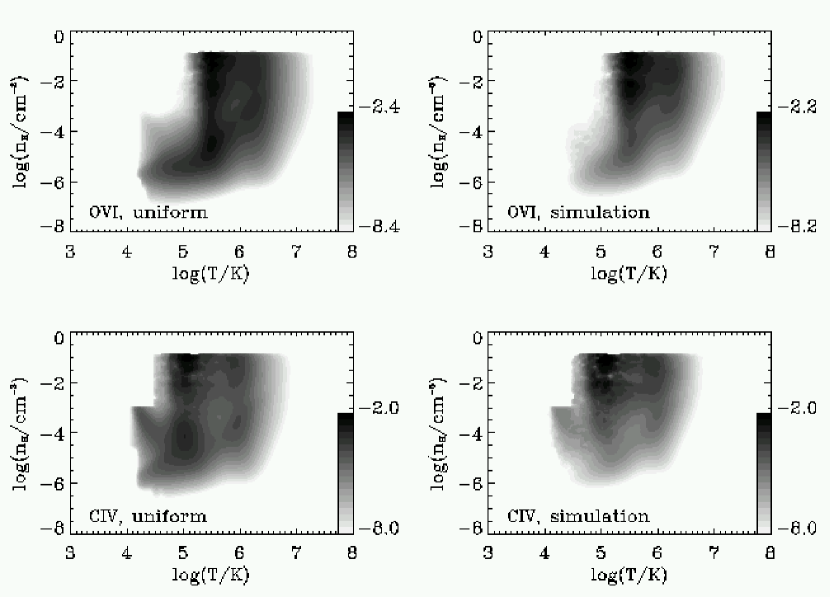
Figure 5.— Distribution of simulation particles in the box at $z=0$. Each panel shows the relative number density of particles in the $n_{\rm H}$–$T$ plane, with a particular weighting. Note that the contours are logarithmic. The top row weights the number density by O VI $\lambda 1032$ emissivity for uniform (upper left) and simulation (upper right) metallicities. The bottom row does the same for the C IV $\lambda 1548$ transition. We have excluded star-forming and self-shielded particles.

4. Results

4.1. Metal Line Maps: Qualitative Features

Figure 4 shows maps of the C IV $\lambda 1548$ and O VI $\lambda 1032$ surface brightness (upper left and upper right, respectively, both assuming simulation metallicities) together with maps of the projected mass-averaged temperature (lower left) and metallicity (lower right) within a slice at $z=0.07$. The redshift width is $\Delta z=0.01$, corresponding to $\Delta\lambda\sim 10$ Åfor O VI $\lambda 1032$; a high spectral resolution instrument would therefore be able to probe considerably narrower redshift slices. All the maps have $\Delta\theta=1\arcmin$ ($\approx 55h^{-1}$ physical kpc at this redshift) and use the metallicities reported by the simulation. Several points are immediately apparent. First, the two transitions trace roughly the same structures: it is rare for a region to emit in one without the other (although this is not necessarily true on a pixel-by-pixel basis), because they both trace warm high-density gas (with $T\sim 10^{5}\mbox{ K}$ for C IV and $T\sim 10^{5.5}\mbox{ K}$ for O VI). Filaments are warmer, denser, and more enriched than the surrounding voids so they stand out clearly in both transitions. This is a simple consequence of the metal dispersal mechanism: winds must begin in galaxies which in turn lie inside overdense regions. (Note, however, that the metallicity is quite inhomogeneous even within filaments.) Second, the O VI maps better trace the diffuse filamentary structure of the IGM. In the C IV maps, filaments appear to be composed of discrete clumps rather than a smooth gas distribution; this transition traces cooler gas that is presumably more tightly associated with galaxies. Finally – and most important – the mean surface brightness of these transitions is extremely small, with O VI $\lambda 1032$ is significantly stronger than C IV $\lambda 1548$ . Given the expected diffuse background ($\gtrsim 10\mbox{ photons cm${}^{-2}$ s${}^{-1}$ sr${}^{-1}$ \AA${}^{-1}$}$ for O VI $\lambda 1032$ and $\gtrsim 100\mbox{ photons cm${}^{-2}$ s${}^{-1}$ sr${}^{-1}$ \AA${}^{-1}$}$ for C IV $\lambda 1548$; see Table 1), only the brightest regions will be visible.

Figure 4 shows that the brightest metal-emitting regions are associated with hot, approximately spherical regions strung along filaments. These regions are heated by two mechanisms. One is structure formation: $T\sim 10^{6}\mbox{ K}$ gas is characteristic of large galaxies and small galactic groups. The large hotspot in the upper left of this map is such a group. A second heat source is galactic winds. In our feedback model, the characteristic temperature of the wind is expected to be $T_{\rm wind}\sim 5\times 10^{6}f_{\rm heat}\mbox{ K}$, where $f_{\rm heat}$ is the fraction of the initial kinetic energy of the wind that remains in thermal energy. Of course, $f_{\rm heat}$ is difficult to calibrate because it depends on cooling within the wind medium (including adiabatic cooling as the wind expands) and on the gravitational potential from which the wind has to escape, but ongoing winds can clearly heat gas to the range relevant for these two transitions. Winds like the ones in our prescription can reach distances $\sim 1h^{-1}\mbox{ Mpc}$ from their host galaxies (Aguirre et al., 2001b), the scale of many of the smaller, nearly spherical hotspots in Figure 4.

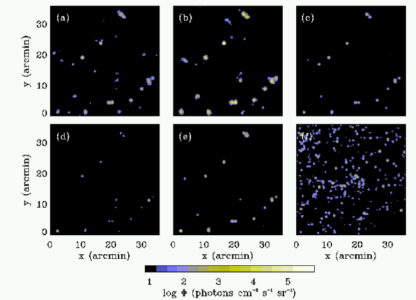
Figure 6.— All the panels except (f) show maps of a $36\arcmin\times 36\arcmin$ slice with $z=0.15$, $\Delta z=0.01$, and $\Delta\theta=0.24\arcmin$. We show only those pixels with $\Phi>7.5\mbox{ photons cm${}^{-2}$ s${}^{-1}$ sr${}^{-1}$}$. (a): O VI $\lambda 1032$ , uniform metallicity. (b): O VI $\lambda 1032$ , simulation metallicity. (c): Ly$\beta$. (d): C IV $\lambda 1548$ , uniform metallicity. (e): C IV $\lambda 1548$ , simulation metallicity. (f): Ly$\alpha$, with the same observed wavelength range as the C IV $\lambda 1548$ panels.

We can better understand the qualitative features of these maps by looking more closely at which particles are luminous. Figure 5 again shows the distribution of particles in the $n_{\rm H}$–$T$ plane, but this time we have weighted the number density by the emission in the separate transitions. The top row weights the density by O VI $\lambda 1032$ emission assuming uniform (left panel) and simulated (right panel) metallicities. The bottom row weights the density by C IV $\lambda 1548$ emissivity. Note the considerable stretch in the colorscale; gas in all but the darkest regions will in fact be unobservable (especially considering that the low-density gas is distributed over a much larger volume). We see in the figure that, in all cases, the total emission comes primarily from a small region within the plane: dense gas in the range $T\sim 10^{5}$–$10^{6}\mbox{ K}$. This is reassuring in two ways. First, a comparison to Figures 1 and 2 shows that the gas responsible for most of the emission is dense enough for its emissivity to be essentially unaffected by the choice of photoionizing background. We thus expect our results to be robust against the uncertainties in the ionizing background. Second, note that O VI $\lambda 1032$ emission from dense gas vanishes for $T\lesssim 10^{5}\mbox{ K}$. Because this is well above our self-shielding threshold (see Figure 3), the location of this cut will have little effect on our predictions about this transition. C IV $\lambda 1548$ emission does extend below the self-shielding threshold (the cut is most visible through the horizontal line at $n_{\rm H}=10^{-3}\mbox{ cm${}^{-3}$}$). However, most self-shielded gas rapidly approaches $T\sim 10^{4}\mbox{ K}$ as it becomes denser; such temperatures are well below the ionization threshold of C IV $\lambda 1548$ and hence the actual emission from self-shielded gas turns out to be small. Furthermore, note that the emission from cooling gas is quite weak in the model with simulation metallicities, so we would not expect self-shielded gas to make as much of a difference in this case.

However, the news is not all positive: a comparison to Figure 3 shows that most of the emission comes from gas lying between the cooling and IGM loci, especially in the simulation metallicity model. The area in which gas emits strongly is only weakly populated in the simulation and hence metal emission is concentrated within rare, bright regions. We also conclude that these transitions are not efficient probes of gas on the standard IGM $n_{\rm H}$–$T$ curve or of the shocked WHIM gas. Finally, comparison of the two different metallicity models shows that a larger fraction of emission comes from gas on the IGM and cooling loci if we assume a uniform metallicity. This is a simple consequence of the metal distribution illustrated in Figure 4: metals tend to be more concentrated inside filaments, which are already relatively bright emitters. A uniform metallicity thus decreases the contrast between filaments and voids.

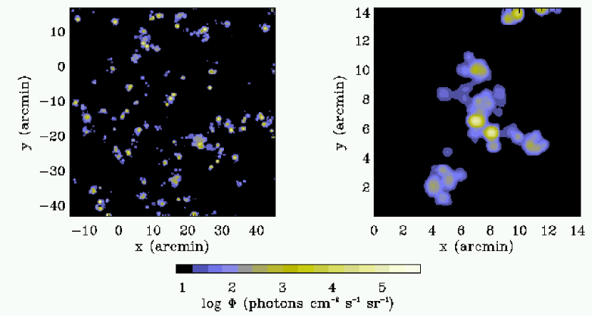
Figure 7.— The left panel shows a $1\arcdeg\times 1\arcdeg$ map of the O VI $\lambda 1032$ transition with $z=0.001$ and $\Delta z=0.16$, including only those pixels with $\Phi>7.5\mbox{ photons cm${}^{-2}$ s${}^{-1}$ sr${}^{-1}$}$. The right panel shows a closeup of a rich section of the larger map. Both maps have $\Delta\theta=0.24\arcmin$. They are constructed assuming simulation metallicities and the HM01 ionizing background.

As mentioned above, nearly all of the emission in Figure 4 is much less than the background and hence unobservable. Figure 6 shows an example of what one could see in a mock (background-limited) observation. Panels (a) through (e) show a slice of the universe with $z=0.15$, $\Delta z=0.01$, and $\Delta\theta=0.24\arcmin$ (corresponding to a physical size $\approx 25h^{-1}\mbox{ kpc}$). Figures 6a and 6b show the surface brightness of the O VI $\lambda 1032$ transition assuming uniform and simulation metallicities, respectively. Figures 6d and 6e show the same for the C IV $\lambda 1548$ transition. We include only those pixels with $\Phi>7.5\mbox{ photons cm${}^{-2}$ s${}^{-1}$ sr${}^{-1}$}$. Table 1 shows that this is a reasonable guess for the diffuse background for O VI $\lambda 1032$, assuming a spectral resolution $\lesssim 1$ Å. It is also compatible with the upper limit of Murthy et al. (1999). However, it underestimates, by at least an order of magnitude, the background redward of Ly$\alpha$ (Brown et al., 2000). It will therefore be extremely difficult to pick out the weaker features shown in the C IV $\lambda 1548$ maps. In all cases, we see that potentially observable emission is confined to isolated bright regions. The number density of such regions is small, particularly for C IV $\lambda 1548$, even though we have chosen a rich region for illustrative purposes. This slice has about three times more bright O VI $\lambda 1032$ regions and six times more bright C IV $\lambda 1548$ regions than average (see §4.3). As expected, the peak brightness increases if we use the simulation metallicities, because these regions are much more enriched than average. We find that the typical sizes of the bright spots are $\sim 80$–$150h^{-1}$ physical kpc for O VI $\lambda 1032$ and $\sim 40$–$50h^{-1}\mbox{ kpc}$ for C IV $\lambda 1548$. Clearly, O VI $\lambda 1032$ emission reveals much more interesting structure than C IV $\lambda 1548$ can.

Figure 7 shows another example of a mock observation. The left panel shows a $1\arcdeg\times 1\arcdeg$ map of the O VI $\lambda 1032$ transition with $\Delta\theta=0.24\arcmin$ and simulation metallicities. We show a full “light cone” from $z=0.001$ to $z=0.16$, illustrating what one could observe with a wide-field integral field spectrometer, and we again include only those pixels with $\Phi>7.5\mbox{ photons cm${}^{-2}$ s${}^{-1}$ sr${}^{-1}$}$. The right panel shows a closeup of a rich section of the larger map. A typical pointing of such an instrument would detect a large number of emission regions. It is also obvious that bright regions are rarely spherical: many features have complex substructure that reflects their internal dynamics.

4.2. Contaminants

As discussed in §2, emission from neutral hydrogen is a potential contaminant in searches for these lines. Figure 6c shows the Ly$\beta$ emission from the same slice as the other panels while Figure 6f shows a different volume corresponding to the same observed wavelength interval as the C IV $\lambda 1548$ panels (placing it at $z=0.47$). Emission from the Ly$\beta$ line is morphologically similar to that from C IV $\lambda 1548$, though it is even more concentrated. Strong Ly$\alpha$ or Ly$\beta$ emission requires a relatively neutral, dense medium and so comes primarily from gas that is near to being self-shielded. The total amount of emission in these lines would have been markedly greater if we had included self-shielded gas, but it would have remained concentrated in isolated objects (see Furlanetto et al. 2003, which contains a detailed discussion of Ly$\alpha$ emission). The probability of a chance superposition of bright C IV $\lambda 1548$ and Ly$\alpha$ emission remains small.

4.3. Pixel Probability Distribution Functions

Figure 8 shows surface brightness information about our maps in a more quantitative form. We have generated an ensemble of 100 maps, each containing $150^{2}$ pixels with $\Delta\theta=0.24\arcmin$, and computed the probability distribution function (PDF) of pixel surface brightness. Here the PDF is defined as $dn/d\ln\Phi$ (with unit normalization). The top and bottom panels show the PDFs of the O VI $\lambda 1032$ and C IV $\lambda 1548$ transitions, respectively. In each panel, we show results assuming both simulated (solid lines) and uniform (dashed lines) metallicities. The dotted curves show the PDF for the surface brightness of Ly$\beta$ at $z=0.15$ (top panel) and Ly$\alpha$ at $z=0.47$ (bottom panel), illustrating the expected background from these transitions. The insets show the bright end of the pixel distribution. We remind the reader that these histograms show only the O VI $\lambda 1032$ and C IV $\lambda 1548$ components of the doublets; the total emission from the doublet is $50\%$ greater than the numbers we quote. On the other hand, if both members of the doublet are required to confirm the reality of a feature, the weaker member fixes the experiment’s sensitivity.

Figure 8.— Pixel surface brightness PDFs in our maps for $z=0.15$ (except Ly$\alpha$, see text), $\Delta z=0.01$, and $\Delta\theta=0.24\arcmin$. The upper and lower panels show the PDFs for the O VI $\lambda 1032$ and C IV $\lambda 1548$ transitions. In each panel, the solid and dashed curves correspond to simulation and uniform metallicities, respectively. The dotted curves show the background from Ly$\beta$ and Ly$\alpha$ transitions (upper and lower panels, respectively). The insets show the bright end of the PDF. All curves assume the HM01 ionizing background.

Bright regions are obviously rare (particularly for C IV $\lambda 1548$), covering only about one percent of the sky in this redshift range. Because the sources are extended, the PDFs do not translate directly into space densities. We find that the comoving density of distinct sources with $\Phi>100\mbox{ photons cm${}^{-2}$ s${}^{-1}$ sr${}^{-1}$}$ is $n_{\rm OVI}\approx 7\times 10^{-3}h^{3}\mbox{ Mpc}^{-3}$ and $n_{\rm CIV}\approx 3\times 10^{-3}h^{3}\mbox{ Mpc}^{-3}$ (assuming simulation metallicities); the difference between the two is less dramatic than suggested by the PDF because O VI $\lambda 1032$ regions are much more extended. Clearly, metallicities from the simulation decrease the surface brightness of the low-density IGM but dramatically increase the number of bright pixels. Luminous regions have recently been enriched by galactic winds and hence have above average metallicity; on the other hand, simulation particles at or below the mean density of the universe have below-average metallicities (because they are far from the galaxies that enrich the IGM). We also see that PDFs calculated from simulation metallicities have broad tails extending toward high surface brightness; these correspond to enriched regions that are moderately overdense and/or outside of the peak temperature range of the transition (i.e., filamentary gas in Figure 6).

Moreover, we find that Ly$\beta$ emission from the low-density IGM is negligible, even compared to that from O VI $\lambda 1032$, but that Ly$\alpha$ emission from this gas dominates the metal lines. The difference between the two hydrogen lines occurs because (1) a much larger fraction of recombinations result in Ly$\alpha$ photons than Ly$\beta$ and (2) the absorption of a $\lambda=1026\mbox{ \AA}$ photon by a neutral hydrogen atom need not result in re-emission of a Ly$\beta$ photon; it can instead be converted to H$\alpha$ and Ly$\alpha$ photons. In the diffuse IGM, this conversion process dominates over the Ly$\beta$ photons produced through recombinations and collisional excitation, so the net emissivity is negligible. The inset shows that pixels are more likely to host Ly$\alpha$ emission than C IV $\lambda 1548$ emission, so having the spectral resolution to resolve both members of each doublet will be crucial to UV metal line emission studies. Contamination by Ly$\alpha$ emission becomes even more severe if we include emission from self-shielded gas (Furlanetto et al., 2003).

As a check on our methods, we now estimate the mean surface brightness of the Ly$\alpha$ transition. We first note that (except in self-shielded regions) the gas is highly photoionized; in this case recombinations dominate over other Ly$\alpha$ production processes. The recombination rate is $\dot{n}_{\rm rec}=\alpha_{\rm H}n_{e}n_{p}$, where $\alpha_{\rm H}$ is the recombination coefficient, and a fraction $\eta\approx 0.42$ of recombinations produce Ly$\alpha$ photons ($\sim 38\%$ of recombinations go directly to the ground state, while $\sim 32\%$ of recombinations to excited states pass through the ²S rather than the ²P state; Osterbrock 1989). The surface brightness per unit wavelength is then (Gould & Weinberg, 1996)

$$\frac{{\rm d}\Phi}{{\rm d}\lambda_{\rm obs}} = \frac{\eta\dot{n}_{\rm rec}}{4\pi(1+z)^{3}}\,\frac{{\rm d}r_{\rm phys}}{{\rm d}z}\,\frac{{\rm d}z}{{\rm d}\lambda_{\rm obs}}$$ (4)

$$\approx 3\times 10^{-3}\left(\frac{\Omega_{b}h^{2}}{0.02}\right)^{2}\frac{(1+z)^{2}}{h(z)}$$

$$\times\delta^{2}h^{-1}\mbox{ photons cm${}^{-2}$ s${}^{-1}$ sr${}^{-1}$ \AA${}^{-1}$},$$

where $h(z)=H(z)/H_{0}$ and $\delta$ represents the effective overdensity of the observed pixel. Given the bandwidth of $\sim 15$ Å in Figure 8, this simple argument reproduces the peak of the Ly$\alpha$ PDF with $\delta\sim 1$, giving us confidence in our analysis procedure. We note that this formula only applies to optically thin absorbing clouds and cannot describe bright pixels in or near the self-shielded regime (Gould & Weinberg, 1996). In principle, a generalization of this formula could be used to estimate the metal line signals as well. However, the temperature-dependent ionization states of oxygen and carbon significantly complicate any such attempt; we can really only extract from it a rough guide to the expected redshift evolution of metal line emission from the low-density IGM.

4.4. Angular Resolution

As mentioned above, O VI $\lambda 1032$ regions have physical scales $\sim 80$–$150h^{-1}\mbox{ kpc}$ and C IV $\lambda 1548$ regions have sizes $\lesssim 40h^{-1}\mbox{ kpc}$. Figures 6 and 7 show that emitting regions can have complex substructure. Typically, O VI $\lambda 1032$ emitters have bright ($\Phi\gtrsim 500\mbox{ photons cm${}^{-2}$ s${}^{-1}$ sr${}^{-1}$}$) central regions of size $\gtrsim 40h^{-1}\mbox{ kpc}$ surrounded by irregular, low surface brightness halos. C IV $\lambda 1548$ regions lack the surrounding halos. Resolving this substructure requires reasonably good angular resolution. We show in Figures 9a and 9b the dependence of the bright tail of the pixel PDF on the instrumental resolution. Each curve is constructed from 100 maps of $150^{2}$ pixels each (after smoothing). The solid, long-dashed, short-dashed, and dotted curves in each panel have $\Delta\theta=1\arcmin,\,0.5\arcmin,\,0.24\arcmin$, and $0.12\arcmin$, respectively (or physical resolutions ranging from $\approx 110h^{-1}\mbox{ kpc}$ to $\approx 13h^{-1}\mbox{ kpc}$, about twice as large as the simulation resolution).

Figure 9.— Pixel PDFs. All curves assume $z=0.15$, $\Delta z=0.01$, simulation metallicities, and the HM01 background unless otherwise specified. (a): The O VI $\lambda 1032$ transition with $\Delta\theta=1\arcmin,\,0.5\arcmin,\,0.24\arcmin$, and $0.12\arcmin$ (solid, long-dashed, short-dashed, and dotted curves, respectively). (b): Same as (a), but for the C IV $\lambda 1548$ transition. (c): The O VI $\lambda 1032$ transition with $z=0.15,\,0.10$, and $0.05$ (solid, dashed, and dotted curves, respectively), with fixed physical resolution of $25h^{-1}\mbox{ kpc}$. (d): PDFs for the HM01s, HM01, HM01w, and HM96 ionizing backgrounds (long-dashed, solid, short-dashed, and dot-dashed curves, respectively) and for no ionizing background (dotted curve), assuming $\Delta\theta=0.24\arcmin$.

We see that the bright tail of the PDF retains qualitatively the same shape, so our conclusions are essentially independent of angular resolution. Increased angular resolution tends to decrease the fraction of moderately bright pixels, by up to an order of magnitude, but increase the peak brightness. The C IV $\lambda 1548$ distribution changes more with $\Delta\theta$ than the O VI $\lambda 1032$ distribution does because C IV $\lambda 1548$ regions tend to be more compact. Resolution effects may begin to saturate at $\Delta\theta<0.24\arcmin$, but this is probably an artifact of being near to the simulation resolution.

4.5. Redshift Evolution

The redshift chosen in our Figures is relatively high; O VI $\lambda 1032$ has nearly redshifted to $1216$ Å, where interference from Ly$\alpha$ will become important. Equation (4) suggests (and our numerical results confirm) that the mean surface brightness of the low-density IGM does not evolve significantly between $z=0$–$0.15$. However, high surface brightness regions are not well-described by equation (4) because they have $\delta>100$. This density regime corresponds to regions that have broken off from the cosmic expansion; such objects should be treated as individual sources. Figure 9c shows the bright end of the O VI $\lambda 1032$ PDF for $z=0.05,\,0.10$, and $0.15$ (dotted, dashed, and solid curves, respectively). We have fixed the physical resolution at each redshift to be $25h^{-1}\mbox{ kpc}$, equivalent to $\Delta\theta=0.24\arcmin$ at $z=0.15$. We see very little evolution with redshift: there is only a slight increase in the number of pixels with a fixed surface brightness as redshift decreases. Although an individual source has a smaller surface brightness as it moves farther from us, the star formation rate increases rapidly with redshift (Springel & Hernquist, 2003b), so there are more (and more powerful) winds at higher redshifts. We find that this effect nearly balances the increasing cosmic distances.

4.6. Ultraviolet Background

Figure 9d shows how the choice of UV background affects the pixel surface brightness distribution. The long-dashed, solid, and short-dashed curves show the PDFs for the O VI $\lambda 1032$ transition assuming the HM01s, HM01, and HM01w backgrounds, respectively. The dotted line assumes pure collisional ionization, while the dot-dashed line assumes the HM96 spectrum. We see that the brightest pixels are essentially independent of the choice of ionizing background. This is to be expected, because the peak emissivity shown in Figure 1 comes from collisionally ionized gas whose location is nearly independent of the background choice. We note that the shape of the low-surface brightness peak does depend on the background: the distribution skews toward higher flux values in weak ionizing backgrounds, because low-density gas is not photoionized to higher states (see Figure 1 and discussion thereof). Although we do not show it, the ionizing background also has no effect on bright C IV $\lambda 1548$ emission.

4.7. Simulation Resolution

Figure 10.— Pixel surface brightness PDFs for $z=0.25$, $\Delta z=0.01$, and a physical resolution of $20h^{-1}\mbox{ kpc}$. The upper and lower panels show the PDFs for the O VI $\lambda 1032$ and C IV $\lambda 1548$ transitions. In each panel, the dotted, solid, and dashed curves correspond to the G4, G5, and G6 runs, respectively. The insets show the bright end of the PDF. All curves assume the HM01 ionizing background.

One important concern is how the resolution of our simulation affects the results. This is particularly important because each bright region has only of order $\sim 10$ bright particles; we therefore do not expect their structure to be fully resolved. Moreover, our wind prescription is stochastic and will not fully capture the dynamics of winds in dwarf galaxies. To estimate the importance of our simulation resolution, we have repeated our analysis for two other simulations, G4 and G6, which are identical to the one described above (G5) except that they contain $144^{3}$ and $486^{3}$ particles, respectively (see Springel & Hernquist 2003b and Nagamine et al. 2003). We show the pixel PDFs for the different simulations in Figure 10; in each panel, the G4, G5, and G6 simulations are shown with dotted, solid, and dashed lines. Both panels assume a uniform metallicity (fixed at that of the G5 run); we have therefore removed the effects of the different metal distribution between the simulations. We see that the simulation resolution has only a small effect on the resulting PDF: in particular, the number of bright pixels increases by only a small amount. We thus conclude that the temperature and density structure of the IGM have converged to good accuracy. The agreement is in fact surprisingly good, given that the G6 simulation resolves large galaxies and winds better but also adds many more small galaxies.

The dependence on resolution in the simulated metallicity case is slightly larger than shown here for the bright pixels, although the change at small surface brightness is non-negligible between the three resolutions. This suggests that the metal distribution does change between the simulations, probably because of the stochastic nature of the enrichment process. If each wind is composed of more particles, any individual volume element in the simulation is more likely to contain such a particle, so the metal distribution is less patchy. We thus find that the G6 simulation has $\sim 25\%$ more pixels with $\Phi\sim 10^{-3}$–$1\mbox{ photons cm${}^{-2}$ s${}^{-1}$ sr${}^{-1}$}$ than the G5 simulation does. The patchiness is not as significant for the brightest regions (where the resolution has about the same effect in both the uniform and simulated metallicity cases), because such regions are compact and the “density” of enriched particles is still large. Thus the stochastic nature of the enrichment process only has an important effect at large distances from the source, where the surface brightness is so low as to be unobservable anyway.

4.8. Angular Correlation Functions

We define the (flux-weighted) correlation function $w(\theta)$ on a pixelized map as (Croft et al., 2001)

$$w(\theta)=\langle\delta_{\Phi}(\bf r)\delta_{\Phi}(\bf{r}+\theta)\rangle,$$ (5)

where $\bf{r}$ is the angular position of a pixel, $\delta_{\Phi}(\bf{r})=\Phi(\bf r)/\bar{\Phi}-1$, and $\bar{\Phi}$ is the mean pixel surface brightness. We measure $w(\theta)$ for each pixel pair of the specified separation and compute the mean value across a given map.

Because spectral line studies automatically contain redshift information, angular clustering statistics such as $w(\theta)$ are perhaps not the optimal measure: one could use the line redshifts to study clustering in three dimensions. However, the angular correlation function is considerably simpler to calculate for a survey geometry such as ours, and we believe it to be adequate for a first approach to the problem. A simple way to retain some redshift information is to compute $w(\theta)$ only for sources within a relatively narrow redshift window. Shot noise will obviously decrease with bandwidth because more sources are included in the map. However, using a large bandwidth would sacrifice all redshift information. We therefore chose to calculate $w(\theta)$ in slices like those described in the previous section. This preserves some redshift information but reduces the shot noise to a manageable level.

Figure 11 shows the angular correlation functions $w(\theta)$ for the O VI $\lambda 1032$ and C IV $\lambda 1548$ transitions (left and right panels, respectively). The solid and dashed curves are the mean correlation function measured from fifty $2.5\arcdeg\times 2.5\arcdeg$ slices with $z=0.15$, $\Delta z=0.01$, and $\Delta\theta=1\arcmin$, assuming simulation and uniform metallicities, respectively. The solid hexagons are the median values (assuming simulation metallicities) measured between maps. The error bars show the upper limits of the first and third quartiles; they illustrate the dispersion in measurements of $w(\theta)$ between individual $2.5\arcdeg\times 2.5\arcdeg$ maps. The solid and open squares show the autocorrelation of the emission; note that the location along the $\theta$-axis is arbitrary because $\theta=0$ does not appear on the logarithmic scale. Because the correlation function is very large for small separations, the top panels show $w(\theta)$ on a logarithmic scale. The correlation rapidly vanishes for larger separations; in order to show this decrease, we plot $w(\theta)$ on a linear scale in the bottom panel.

Figure 11.— Angular correlation function for the O VI $\lambda 1032$ (left) and C IV $\lambda 1548$ (right) transitions in slices with $z=0.15$, $\Delta z=0.01$, and $\Delta\theta=1\arcmin$. The upper and lower panels show $w(\theta)$ in logarithmic and linear units, respectively. The solid and dashed curves show the mean signal for the simulation and uniform metallicity models, respectively. The hexagonal points are the median values of $w(\theta)$ and the error bars show the upper limits of the first and third quartiles (assuming simulation metallicities). The solid and open squares show the autocorrelation of the maps for simulation and uniform metallicities, respectively.

Metal line emission is clearly clustered: $w(\theta=7.5\arcmin)\sim 1$ for O VI $\lambda 1032$ and $w(\theta=5\arcmin)\sim 1$ for C IV $\lambda 1548$, corresponding to physical separations of $\sim 800h^{-1}\mbox{ kpc}$ and $\sim 550h^{-1}\mbox{ kpc}$, respectively. A power law of index $n\sim 3.5$ ($n\sim 4$) adequately fits the correlation function for O VI $\lambda 1032$ (C IV $\lambda 1548$). The correlation function is much steeper than that of galaxies, at least partly because we have weighted the pixels by their fluxes. A difference from galaxies is not surprising because of the complicated physics behind line emission: there is no reason to expect the line emission to correspond to bright galaxies. Rather, emission is likely to come from those galaxies that (for whatever reason) host an ongoing wind. Note that the correlation length we measure is approximately the size of galactic winds (see Figure 4 and discussion thereof).

The case with simulation metallicities is somewhat more strongly clustered at small scales because of the metallicity gradient between enriched, emitting regions and the (relatively) pristine, low-density IGM. However, differentiating the two through clustering will be difficult because the dispersion between maps is nearly as large as the difference between the two models. Cosmic variance is also very large, because the correlation function is dominated by rare, bright pixels. Comparison of the mean and median shows that a typical map underestimates the true correlation coefficient, particularly at intermediate scales. This is because the positive part of the signal is dominated by pairs of bright pixels, for which the probability is quite small. Thus, a precise measurement of the clustering properties of metal line emitters will require a survey over a large volume.

We have not included any background emission in this calculation of $w(\theta)$ because (as discussed above) the background level at these wavelengths is so uncertain. However, computing the correlation function directly from the raw map (without background subtraction) smooths the correlation substantially because the total flux from a map of this size is dominated not by the metal emitters but by the background radiation field. A better strategy is to set all pixels below a certain signal-to-noise to zero. This procedure does not decrease the number of individual sources by much, because most contain bright cores well above the background.

5. Discussion

We have examined the emission expected from the IGM in two UV metal line doublets, O VI $\lambda\lambda 1032,1038$ and C IV $\lambda\lambda 1548,1551$. Using state-of-the-art cosmological simulations that include prescriptions for star formation and galactic winds, we computed the surface brightness distribution of these lines. We assume the IGM to be photoionized by a diffuse background, and we include several different models for this (currently uncertain) background radiation. We also considered two different metallicity distributions for the IGM: a uniform metallicity model and a model with the metallicities predicted by our simulation (essentially including winds from galaxies at low and moderate redshifts).

Can UV metal line emission from the IGM plausibly be observed? A comparison of Table 1 and Figure 8 shows that, in the low-density IGM, the emission from either of our transitions is several orders of magnitude smaller than that of any realistic background radiation; we therefore conclude that these transitions provide little information about the “missing baryons” (i.e., baryons with high temperatures but low densities). Instead, Figures 4 and 6 show bright emission is concentrated into isolated regions with (1) significantly higher metallicity than the average, (2) $T\sim 10^{5}\mbox{ K}$ (for C IV $\lambda 1548$) or $T\sim 10^{5.5}\mbox{ K}$ (for O VI $\lambda 1032$), and (3) a density much greater than the cosmic mean. C IV $\lambda 1548$ emission is generally confined to compact regions of size $\lesssim 40h^{-1}\mbox{ kpc}$, while O VI $\lambda 1032$ emission is generally more extended with bright central cores of size $\sim 50h^{-1}\mbox{ kpc}$ surrounded by weaker, irregular halos. The overall space density of emitting regions is $n_{\rm OVI}\approx 7\times 10^{-3}h^{3}\mbox{ Mpc}^{-3}$ and $n_{\rm CIV}\approx 3\times 10^{-3}h^{3}\mbox{ Mpc}^{-3}$ (comoving) at $z=0.15$. Overall, we find that O VI $\lambda 1032$ has more promise as an observational probe.

Detection of metal line emission is feasible (but challenging) with existing technology. The ideal instrument for these observations would be an integral field spectrograph with a large field of view; resolution of at least $\sim 10\arcsec$ would be necessary to study the detailed structure of the sources. Existing instruments do not meet these criteria, though the next generation of instruments probably will. The Galaxy Evolution Explorer (GALEX), with a large field of view but relatively low spectral resolution ($\sim 10$ Å), may detect the brightest cores, though its poor spectral resolution would make it impossible to identify doublets unambiguously. A project underway to construct a balloon-borne wide-field UV spectrograph will have a limiting sensitivity $\Phi\sim 500\mbox{ photons cm${}^{-2}$ s${}^{-1}$ sr${}^{-1}$}$ in a single night’s observation (D. Schiminovich, private communication); such an instrument could detect the cores of many O VI emitting regions. Finally, the proposed Spectroscopy and Photometry of the IGM’s Diffuse Radiation would have the sensitivity to detect the bright cores. Background-limited observations to detect emission on $\sim 100\mbox{ kpc}$ scales will require a much larger collecting area than currently planned for any wide-field instrument. High spectral resolution would help to reduce the background, which is especially important for observations redward of $1216$ Å.

Comparison of the topology of luminous regions to the temperature and metallicity distribution in the IGM (see Figure 4) shows that most bright particles are embedded in hot ($T\gtrsim 10^{6}\mbox{ K}$) enriched regions characteristic of galaxy groups and winds. We therefore suggest that these transitions probe models of metal enrichment and galactic feedback. We have shown that these observations can distinguish a uniform IGM metallicity from one in which the metals are dispersed by powerful winds. If mixing is more efficient than the simulation allows, the emission could be more extended than we predict but have smaller peak luminosities. Unfortunately, the feedback parameters in our simulation model are fixed, and we are thus unable to investigate how the emission varies with them. We have deliberately chosen an extreme wind model (in which none of the supernova energy is lost to radiative cooling before powering the wind). Metal emission will tend to be more compact if winds have less energy simply because they cannot penetrate as much of the IGM. However, a more subtle consequence of our choice is that it allows all of the supernova energy to heat the wind medium. Weaker winds may therefore lead to more emission, because the wind stays cooler near to the host galaxy; however, note that the wind velocity of our model is consistent with observations (Martin, 1999).

It is important to note that the extent of observable O VI $\lambda 1032$ and (especially) C IV $\lambda 1548$ emission does not trace out the extent of metal enrichment. Collisional excitation of these lines requires high density and $T\gtrsim 10^{5}\mbox{ K}$. As winds expand into the IGM, their density decreases rapidly and thermal energy injected by the wind is lost to cooling. Thus we would expect emission from wind-enriched regions to fade with time. The declining star formation rate at low redshifts implies that active winds become relatively rare in the local universe. Most enrichment occurred at earlier epochs, giving the winds time to expand and mix with the surrounding IGM. Nevertheless, observations of line emission will provide a census of enriched, warm regions at the present day.

Higher resolution observations of individual sources have the potential to teach us about the structure of galactic winds. If viewed in O VI $\lambda 1032$ emission, we predict a central, bright core surrounded by an irregular, low surface brightness halo. However, the actual structure will be much more complex than our simulation, with its relatively coarse resolution, can accurately describe. Real galactic winds have extremely complicated internal structures with several different temperature phases that can be separated through observations of diffuse X-ray gas with $kT\gtrsim 0.1\mbox{ keV}$ (e.g., Strickland et al. 2000), absorption lines of low-ionization species (such as Na I; Heckman et al. 2000), and both emission lines (like H$\alpha$; Martin 1998) and absorption lines (Shapley et al., 2003) typical of highly ionized regions. These are thought to probe, respectively, a hot phase with large filling factor, a cool phase made up of embedded clouds, and a warm phase on the interface between the two (Heckman, 2002). This last phase should host O VI $\lambda 1032$ and C IV $\lambda 1548$ emission. Recent observations of the wind surrounding M82, a nearby starburst galaxy, show that O VI $\lambda 1032$ is not an efficient coolant of gas within several kiloparsecs of the host galaxy (Hoopes et al., 2003); however, the limiting surface brightness ($\Phi\lesssim 10^{5}\mbox{ photons cm${}^{-2}$ s${}^{-1}$ sr${}^{-1}$}$ for this nearby system) is compatible with our predictions. Because of the many observational mysteries, metal lines offer a powerful probe of galactic winds complementary to existing techniques. In particular, emission line observations, which can in principle probe scales up to $\sim 100\mbox{ kpc}$, will help to determine how winds evolve on scales large compared to their host galaxies. Correlating the line emission maps to galaxy surveys will teach us about the properties of galaxies that are able to drive powerful winds and by extension the types of galaxies responsible for enriching the IGM with metals.

Our predictions are subject to several important uncertainties. First, we have excluded self-shielded and star-forming gas from our analysis. Self-shielded gas is unlikely to contribute significantly to O VI $\lambda 1032$ emission, because it is much too cool, but it could add a small number of additional C IV $\lambda 1548$ sources. Self-shielding is significantly more important for studies of hydrogen line transitions (Furlanetto et al., 2003), because dense, cool clumps of gas show strong Ly$\alpha$ and Ly$\beta$ lines. A high enough spectral resolution to resolve the O VI and C IV doublets will be necessary to prevent contamination. Galaxies will inevitably be strong emitters at these wavelengths and present another potential source of confusion for studies of the IGM. However, they can be removed from maps like the ones we show because they will also be strong continuum emitters, provided that the angular resolution of the instrument is smaller than the size of the emitting regions.

Another set of caveats has to do with the simulation itself. The most obvious is its finite resolution. However, we showed in §4.7 that the density and temperature structure of our simulation has converged. The remaining uncertainty is in the patchiness of the metal distribution, but that has little effect on the bright regions. Another concern is that the simulation neglected metal line cooling. We argued in §3.1 that this is probably only important in highly enriched regions such as winds. We expect it to decrease the number density of bright regions by, at most, a factor of a few, and to increase their surface brightness (because they cool through the relevant temperature regime sooner). Note that Hoopes et al. (2003) argue that line cooling is not important for winds within $\sim 10\mbox{ kpc}$ of the host galaxy.

Finally, we neglected local effects such as dust and variations in the background radiation field. Because luminous regions tend to be quite dense, the local radiation field likely will not strongly affect our results. Most important, we find that the bright end of the pixel distribution is largely unaffected by uncertainty in the ionizing background (see Figure 9d), although ionizing radiation from the host galaxy of a wind could still have substantial effects. Dust is a particular concern because galactic winds have been observed to carry it over sizable distances (Heckman et al., 2000); much of our emission comes from regions recently enriched by winds, so dust will likely decrease the emissivity of such regions. Fortunately the measured extinction in local starburst winds is usually not large and may be patchy, so we expect our qualitative results to remain unchanged.

Despite these uncertainties, our results show that C IV $\lambda 1548$ and especially O VI $\lambda 1032$ emission can be detected from the IGM. While emission from the low density “missing baryons” is too weak to be detected, we find that observations of these transitions may distinguish different enrichment patterns in the IGM; they thus offer one of the few methods to probe the effects of mechanical, wind-driven feedback from galaxies. Many of the uncertainties we have mentioned have to do with the detailed structure and mechanism of winds; observations of the metal emission will of course help to resolve these questions. When combined with observations of emission from higher ionization states (such as O VII and O VIII; Yoshikawa et al. 2003), maps of the UV doublets we have studied will also teach us about the thermal structure of the enriched IGM, offering an even more complete picture of the wind mechanism.

References

- Aguirre et al. (2001a) Aguirre, A., et al. 2001a, ApJ, 556, L11
- Aguirre et al. (2001b) —. 2001b, ApJ, 560, 599
- Anders & Grevesse (1989) Anders, E., & Grevesse, N. 1989, Geochim. Cosmochim. Acta, 53, 197
- Aracil et al. (2003) Aracil, B., et al. 2003, ApJ, submitted (astro-ph/0307506)
- Bi (1993) Bi, H. 1993, ApJ, 405, 479
- Bi et al. (1992) Bi, H. G., Boerner, G., & Chu, Y. 1992, A&A, 266, 1
- Bromm et al. (2001) Bromm, V., Ferrara, A., Coppi, P. S., & Larson, R. B. 2001, MNRAS, 328, 969
- Bromm et al. (2003) Bromm, V., Yoshida, N., & Hernquist, L. 2003, ApJ, 596, L135
- Brown et al. (2000) Brown, T. M., et al. 2000, AJ, 120, 1153
- Carswell et al. (2002) Carswell, B., Schaye, J., & Kim, T. 2002, ApJ, 578, 43
- Cen (2003) Cen, R. 2003, ApJ, 591, 12
- Cen et al. (1994) Cen, R., Miralda-Escudé, J., Ostriker, J. P., & Rauch, M. 1994, ApJ, 437, L9
- Cen & Ostriker (1999) Cen, R., & Ostriker, J. P. 1999, ApJ, 514, 1
- Cowie & Songaila (1998) Cowie, L. L., & Songaila, A. 1998, Nature, 394, 44
- Cowie et al. (1995) Cowie, L. L., Songaila, A., Kim, T., & Hu, E. M. 1995, AJ, 109, 1522
- Croft et al. (2001) Croft, R. A. C., et al. 2001, ApJ, 557, 67
- Davé et al. (1999) Davé, R., Hernquist, L., Katz, N., & Weinberg, D. H. 1999, ApJ, 511, 521
- Davé & Tripp (2001) Davé, R., & Tripp, T. M. 2001, ApJ, 553, 528
- Davé et al. (1998) Davé, R., et al. 1998, ApJ, 509, 661
- Davé et al. (2001) —. 2001, ApJ, 552, 473
- Dekel & Silk (1986) Dekel, A., & Silk, J. 1986, ApJ, 303, 39
- Dixon et al. (2001) Dixon, W. V. D., Sallmen, S., Hurwitz, M., & Lieu, R. 2001, ApJ, 552, L69
- Edelstein et al. (2000) Edelstein, J., Bowyer, S., & Lampton, M. 2000, ApJ, 539, 187
- Ellison et al. (2000) Ellison, S. L., Songaila, A., Schaye, J., & Pettini, M. 2000, AJ, 120, 1175
- Ferland (2000) Ferland, G. J. 2000, in Revista Mexicana de Astronomia y Astrofisica Conference Series, 153–157
- Ferland (2001) Ferland, G. J. 2001, Hazy, A Brief Introduction to Cloudy 94.00 (http://www.pa.uky.edu/ gary/cloudy/)
- Furlanetto & Loeb (2003) Furlanetto, S. R., & Loeb, A. 2003, ApJ, 588, 18
- Furlanetto et al. (2003) Furlanetto, S. R., Schaye, J., Springel, V., & Hernquist, L. 2003, ApJ, 599, L1
- Gould & Weinberg (1996) Gould, A., & Weinberg, D. H. 1996, ApJ, 468, 462
- Haardt & Madau (1996) Haardt, F., & Madau, P. 1996, ApJ, 461, 20 [HM96]
- Haardt & Madau (2001) Haardt, F., & Madau, P. 2001, in Clusters of Galaxies and the High Redshift Universe Observed in X-rays, ed. D. M. Neumann & J. T. T. Van (21st Moriond Astrophysics Meeting, Les Arc, France) [HM01]
- Heckman (2002) Heckman, T. M. 2002, in ASP Conf. Ser. 254: Extragalactic Gas at Low Redshift, ed. J. Mulchaey and J. Stocke (San Francisco: ASP), 292
- Heckman et al. (2000) Heckman, T. M., Lehnert, M. D., Strickland, D. K., & Armus, L. 2000, ApJS, 129, 493
- Hellsten et al. (1998) Hellsten, U., Gnedin, N. Y., & Miralda-Escudé, J. 1998, ApJ, 509, 56
- Hernquist (1993) Hernquist, L. 1993, ApJ, 404, 717
- Hernquist et al. (1996) Hernquist, L., Katz, N., Weinberg, D. H., & Jordi, M. 1996, ApJ, 457, L51
- Hernquist & Springel (2003) Hernquist, L., & Springel, V. 2003, MNRAS, 341, 1253
- Hoopes et al. (2003) Hoopes, C. G., Heckman, T. M., Strickland, D. K., & Howk, J. C. 2003, ApJ, 596, L175
- Hui & Gnedin (1997) Hui, L., & Gnedin, N. Y. 1997, MNRAS, 292, 27
- Katz et al. (1996) Katz, N., Weinberg, D. H., & Hernquist, L. 1996, ApJS, 105, 19
- Lehnert & Heckman (1996) Lehnert, M. D., & Heckman, T. M. 1996, ApJ, 462, 651
- Mackey et al. (2003) Mackey, J., Bromm, V., & Hernquist, L. 2003, ApJ, 586, 1
- Madau et al. (2001) Madau, P., Ferrara, A., & Rees, M. J. 2001, ApJ, 555, 92
- Martin (1998) Martin, C. L. 1998, ApJ, 506, 222
- Martin (1999) —. 1999, ApJ, 513, 156
- McDonald et al. (2001) McDonald, P., et al. 2001, ApJ, 562, 52
- Murthy et al. (1999) Murthy, J., Hall, D., Earl, M., Henry, R. C., & Holberg, J. B. 1999, ApJ, 522, 904
- Nagamine et al. (2003) Nagamine, K., Springel, V., Hernquist, L., & Machacek, M., MNRAS, submitted (astro-ph/0311295)
- Oh et al. (2001) Oh, S. P., Nollett, K. M., Madau, P., & Wasserburg, G. J. 2001, ApJ, 562, L1
- Osterbrock (1989) Osterbrock, D. E. 1989, Astrophysics of Gaseous Nebulae and Active Galactic Nuclei (Mil Valley, CA: Univ. Sci.)
- Otte et al. (2003) Otte, B., Dixon, W. V., & Sankrit, R. 2003, ApJ, 586, L53
- Perna & Loeb (1998) Perna, R. & Loeb, A. 1998, ApJ, 503, L135
- Pettini et al. (2001) Pettini, M., et al. 2001, ApJ, 554, 981
- Pettini et al. (2002) —. 2002, ApJ, 569, 742
- Pieri & Haehnelt (2003) Pieri, M. M., & Haehnelt, M. G. 2003, MNRAS, submitted (astro-ph/0308003)
- Schaye (2001) Schaye, J. 2001, ApJ, 559, 507
- Schaye et al. (2000) Schaye, J., Rauch, M., Sargent, W. L. W., & Kim, T. 2000, ApJ, 541, L1
- Schaye et al. (1999) Schaye, J., Theuns, T., Leonard, A., & Efstathiou, G. 1999, MNRAS, 310, 57
- Schaye et al. (2003) Schaye, J., et al. 2003, ApJ, 596, 768
- Shapley et al. (2003) Shapley, A. E., Steidel, C. C., Pettini, M., & Adelberger, K. L. 2003, ApJ, 588, 65
- Shelton et al. (2001) Shelton, R. L., et al. 2001, ApJ, 560, 730
- Sokasian et al. (2003) Sokasian, A., Abel, T., Hernquist, L., & Springel, V. 2003, MNRAS, 344, 607
- Songaila & Cowie (1996) Songaila, A., & Cowie, L. L. 1996, AJ, 112, 335
- Spergel et al. (2003) Spergel, D. N., et al. 2003, ApJS, 148, 175
- Springel & Hernquist (2002) Springel, V., & Hernquist, L. 2002, MNRAS, 333, 649
- Springel & Hernquist (2003a) —. 2003a, MNRAS, 339, 289
- Springel & Hernquist (2003b) —. 2003b, MNRAS, 339, 312
- Springel et al. (2001a) Springel, V., White, M., & Hernquist, L. 2001a, ApJ, 549, 681
- Springel et al. (2001b) Springel, V., Yoshida, N., & White, S. D. M. 2001b, New Astronomy, 6, 79
- Strickland et al. (2000) Strickland, D. K., Heckman, T. M., Weaver, K. A., & Dahlem, M. 2000, AJ, 120, 2965
- Theuns et al. (1998) Theuns, T., et al. 1998, MNRAS, 301, 478
- Tripp et al. (2000) Tripp, T. M., Savage, B. D., & Jenkins, E. B. 2000, ApJ, 534, L1
- Tytler et al. (1995) Tytler, D., et al. 1995, in QSO Absorption Lines, Proceedings of the ESO Workshop, ed. G. Meylan (Berlin: Springer), 289
- Welsh et al. (2002) Welsh, B. Y., et al. 2002, A&A, 394, 691
- Wyithe & Loeb (2003a) Wyithe, J. S. B., & Loeb, A. 2003a, ApJ, 586, 693
- Wyithe & Loeb (2003b) —. 2003b, ApJ, 588, L69
- Yoshikawa et al. (2003) Yoshikawa, K., et al. 2003, PASJ, 55, 879
- Zhang et al. (1995) Zhang, Y., Anninos, P., & Norman, M. L. 1995, ApJ, 453, L57