Mass and Angular Momentum Transfer
in the Massive Algol Binary RY Persei

Abstract

We present an investigation of H$\alpha$ emission line variations observed in the massive Algol binary, RY Per. We give new radial velocity data for the secondary based upon our optical spectra and for the primary based upon high dispersion UV spectra. We present revised orbital elements and an estimate of the primary’s projected rotational velocity (which indicates that the primary is rotating $7\times$ faster than synchronous). We use a Doppler tomography algorithm to reconstruct the individual primary and secondary spectra in the region of H$\alpha$, and we subtract the latter from each of our observations to obtain profiles of the primary and its disk alone. Our H$\alpha$ observations of RY Per show that the mass gaining primary is surrounded by a persistent but time variable accretion disk. The profile that is observed outside-of-eclipse has weak, double-peaked emission flanking a deep central absorption, and we find that these properties can be reproduced by a disk model that includes the absorption of photospheric light by the band of the disk seen in projection against the face of the star. We developed a new method to reconstruct the disk surface density distribution from the ensemble of H$\alpha$ profiles observed around the orbit, and this method accounts for the effects of disk occultation by the stellar components, the obscuration of the primary by the disk, and flux contributions from optically thick disk elements. The resulting surface density distribution is elongated along the axis joining the stars, in the same way as seen in hydrodynamical simulations of gas flows that strike the mass gainer near trailing edge of the star. This type of gas stream configuration is optimal for the transfer of angular momentum, and we show that rapid rotation is found in other Algols that have passed through a similar stage.

1 Introduction

Algol-type binary systems consist of a hot, B-A main sequence primary star and a cool, less massive F-K giant or subgiant secondary companion in a close orbit (Peters, 1989, 2001). They appear to have formed from previously detached binaries in which the originally more massive star (now the secondary) evolves off the main sequence, expands to its Roche lobe limit, and begins to transfer mass and angular momentum to its companion (the primary). The gas stream from the donor to the gainer follows a path that directly strikes the star in short period systems while in longer period systems ($P>6$ d) the stream misses the star and forms an accretion disk. The circumstellar gas is observed in UV and optical emission lines, and the H$\alpha$ line in particular has served as an important diagnostic of the outflow (Richards & Albright, 1999; Richards, 2001). H$\alpha$ profiles corrected for photospheric absorption show single and/or double-peaked emission features at most orbital phases. Richards & Albright (1999) have made Doppler tomographic reconstructions of the H$\alpha$ emission in many systems, and these tomograms are important diagnostics in searching for evidence of the gas streams and disks.

RY Persei (HD 17034 = HIP 12891 = BD$+47^{\circ}692$) is a remarkable example of one of the most massive Algol binaries. In a seminal paper Olson & Plavec (1997) determined accurate values of the masses and radii of this totally eclipsing system ($P=6.86$ d): $M_{P}/M_{\odot}=6.25\pm 0.16$ and $R_{P}/R_{\odot}=4.06\pm 0.14$ for the B4: V gainer and $M_{S}/M_{\odot}=1.60\pm 0.10$ and $R_{S}/R_{\odot}=8.10\pm 0.17$ for the F7: II-III donor star. Olson & Plavec (1997) discuss the ample evidence for ongoing mass transfer and circumstellar gas, and they point out that the gainer is rotating approximately $10\times$ faster than the orbital synchronous rate. Thus, RY Per offers us a key opportunity to investigate the process of mass transfer and the resulting spin up of the gainer in a system with well known properties. We are particularly interested in learning whether or not this process of spin up is a possible explanation for the origin of the Be and other rapidly rotating massive stars (Gies et al., 1998; Gies, 2001).

Here we present the results of an investigation of new high quality H$\alpha$ spectroscopy of RY Per obtained with the Kitt Peak National Observatory (KPNO) Coude Feed Telescope. In §2 we describe the observations (which include two intensive series of spectra obtained in 1999 October and 2000 October during total eclipses of the primary) and new radial velocity data for the secondary. We also present radial velocities for the primary derived from high dispersion UV spectroscopy made with the International Ultraviolet Explorer Satellite (IUE). We present revised orbital elements in §3 and discuss the projected rotational velocity of the primary in §4. We show the results of a Doppler tomographic reconstruction of the stellar component spectra in §5, where we also discuss the removal of the secondary’s spectrum from the composite spectra. We present in §6 a disk model of the time- and orbital phase-averaged H$\alpha$ profile using the method of Hummel & Vrancken (2000) that is applicable to Be “shell” stars. Our study indicates, however, that there is evidence of non-axisymmetric structure in the disk of RY Per, and in §7 we present a new method to reconstruct the disk surface density distribution from the H$\alpha$ observations. We summarize our results in §8 and discuss how RY Per is representative of Algol systems at a stage where the angular momentum transfer efficiency peaks.

2 Observations and Radial Velocity Measurements

The optical spectra were obtained with the KPNO 0.9-m Coude Feed Telescope during four runs between 1999 October and 2000 October. A summary of the different observing runs is given Table 1 which lists the beginning and ending UT dates of observation, grating, filter, spectral resolving power ($\lambda/\delta\lambda$), and wavelength range recorded. In the first two runs we used the short collimator, grating BL181, and camera 5 with a Ford $3072\times 1024$ CCD (F3KB) as the detector. During the third and fourth runs we used the same camera and detector but changed to the long collimator with higher dispersion gratings (gratings A and B in the third and fourth runs, respectively). Exposure times were generally 30 minutes, which produced a signal-to-noise ratio of $S/N\approx 300$ in the lower dispersion, out-of-eclipse spectra. We also observed with each configuration the rapidly rotating A-type star, $\zeta$ Aql, which we used for removal of atmospheric water vapor lines. Each set of observations was accompanied by numerous bias and flat field frames, and wavelength calibration frames of a Th Ar comparison lamp were obtained at approximately 90 minute intervals each night.

The spectra were extracted and calibrated using standard routines in IRAF. All the spectra were rectified to a unit continuum by fitting line-free regions. The removal of atmospheric lines was done by creating a library of $\zeta$ Aql spectra from each run, removing the broad stellar features from these, and then dividing each target spectrum by the modified atmospheric spectrum that most closely matched the target spectrum in a selected region dominated by atmospheric absorptions. The spectra from each run were then transformed to a common heliocentric wavelength grid.

We measured radial velocities for the secondary by cross correlating each spectrum with a mid-eclipse spectrum (from HJD 2,451,463.804) that is dominated by the secondary’s flux. We omitted from the calculation those spectral regions containing strong interstellar and primary star lines. Radial velocities were obtained by fitting a parabola to the cross correlation function extremum. Note that there is no problem in using a lower resolution spectral template (from the first run) in forming cross correlation functions with higher resolution spectra (from the third and fourth runs), since the degraded resolution simply broadens the cross correlation function but does not affect its central position. We transformed these relative velocities to an absolute scale by measuring the cross correlation shift between the mid-eclipse reference spectrum and a spectrum we made of HD 216228 (K0 III) which has a radial velocity of $-14.2\pm 0.7$ km s^-1 (Barbier-Brossat & Figon, 2000). We observed this radial velocity standard star in all but the third run, and cross correlation measurements indicate that any systematic errors between the runs are negligible ($<1.4$ km s^-1). Our final results are presented in Table 2, which lists the heliocentric Julian date of mid-exposure, the spectroscopic orbital phase (§3), the radial velocity, and the observed minus calculated radial velocity residual (§3).

The He I $\lambda\lambda 5876,6678$ lines of the primary appear to be partially blended with lines from the secondary and circumstellar components, so they are not suitable for measuring the orbital motion of the primary. Instead we measured radial velocities of the primary in the spectral range 1240 – 1850 Å recorded in International Ultraviolet Explorer Satellite high dispersion, short wavelength prime camera spectra. The secondary has negligible flux in this spectral region. We obtained radial velocities by cross correlating each spectrum with the narrow-lined spectrum of $\iota$ Her (B3 IV), which has a radial velocity of $-20.0$ km s^-1 (Abt & Levy, 1978). Here we omitted rom the calculation any spectral regions containing strong interstellar and circumstellar lines. Our measured absolute radial velocities for the primary are collected in Table 3 (in the same format as Table 2).

3 Revised Orbital Elements

The last spectroscopic orbital solution was made by Popper (1989), and we decided it was worthwhile to check the period and orbital elements with the new data. We first determined times of primary mid-eclipse from our intensive spectroscopic coverage of two eclipses by finding the times of maximum secondary line depth (HJD $2451463.817\pm 0.020$ and $2451820.731\pm 0.020$). Both of these times are consistent with the primary eclipse ephemeris of Olson & Plavec (1997) and of Kreiner et al. (2001), so we adopted in our radial velocity analysis the orbital period assumed by Olson & Plavec (1997), $P=6.863569$ d, which is based on the analysis by Van Hamme & Wilson (1986) of photometry by Popper & Dumont (1977).

The radial velocity curve of the secondary can be determined much more accurately than that of the primary because the measurement errors are smaller (more and narrower lines) and because we have more measurements. We determined orbital elements for both stars using the non-linear least-squares fitting code of Morbey & Brosterhus (1974). We first solved for the five orbital elements for the secondary: eccentricity ($e$), longitude of periastron ($\omega_{S}$), semiamplitude ($K_{S}$), systemic velocity ($V_{S}$), and time of periastron ($T_{S}$). The fit of the primary radial velocities was made by fixing $e$, $\omega_{P}=\omega_{S}+180^{\circ}$, and $P$ using the secondary’s solution. The resulting orbital elements are listed in Table 4 (together with those from Popper (1989)) and the radial velocity curve and observations are shown in Figure 1. The difference in the systemic velocity between the solutions for the primary and secondary is probably not significant given the very different ways in which the radial velocities were measured in the UV and optical spectra. The masses and semimajor axis were calculated using $i=83\fdg 0$ (Olson & Plavec, 1997).

Our results are in good agreement with those of Popper (1989). The main difference is our finding that the eccentricity is significantly different from zero, and this is somewhat surprising given that most Roche lobe overflow systems have circular orbits. However, Algol itself has a small but non-zero eccentricity (Hill et al., 1971), which may be related to the presence of a distant third star (Donnison & Mikulskis, 1995). A statistical test of the significance of a non-zero eccentricity in RY Per was made following Lucy & Sweeney (1971) by evaluating the probability that the reduction in the error of the fit through the addition of two parameters in an elliptical solution ($e,\omega$) could have exceeded that obtained, i.e.,

$$p=(R_{e}/R_{c})^{\beta}$$

where $R_{e}$ is the sum of the squares of the residuals for an elliptical fit, $R_{c}$ is the same for a circular fit, $\beta=(N-M)/2$, $N$ is the number of observations, and $M$ is the number of fitting parameters ($M=5$ since the period $P$ was set independently). We found that the r.m.s. of the fit dropped from 5.1 km s^-1 for a circular fit to 3.4 km s^-1 for an elliptical fit, and the probability that such an improvement would occur by random errors is $p=10^{-8}$. For the remainder of this paper we will refer to the photometric convention for orbital phase (0 at primary eclipse), $\phi_{\rm phot}=\phi_{\rm spec}-0.541$.

4 Projected Rotational Velocity of the Primary

We measured the projected rotational broadening of the primary’s UV lines following the method of Howarth et al. (1997). This method uses the width of the cross correlation function (ccf) discussed in §2 as a measure of the photospheric line broadening (which is dominated by rotational broadening for the UV lines included in the construction of the ccf). First the UV reference spectrum of $\iota$ Her was cross correlated with itself to produce a sharp autocorrelation whose width measures the thermal broadening of the lines and any systematic effects due to line blending. We then assumed that the observed ccf was a convolution of the $\iota$ Her autocorrelation function (for $V\sin i=0$; Abt et al. (2002)) with a simple rotational broadening function based upon a linear limb darkening coefficient (Gray, 1992). The limb darkening coefficient was taken from the tables of Wade & Rucinski (1985) using the stellar effective temperature and gravity given by Olson & Plavec (1997). The best fit of the broadened autocorrelation with the observed ccf occurred for $V\sin i=213\pm 10$ km s^-1, which is in good agreement with the value of $V\sin i=212\pm 7$ km s^-1 found by Etzel & Olson (1993) from optical lines. This implies that the primary is spinning $(7.2\pm 0.3)\times$ faster than the synchronous rate (given the stellar radius and system inclination from Olson & Plavec (1997)).

5 Spectral Components and H$\alpha$ Emission

Our primary focus in this paper is the H$\alpha$ emission flux that is formed in the vicinity of the hot primary star. However, the cool secondary star’s spectrum also displays many line features in this same spectral region (including H$\alpha$ in absorption). Thus, we need to remove the secondary star’s spectral contribution from the observed spectra in order to study the H$\alpha$ contributions from the primary star and its circumstellar gas.

There are many approaches to finding a suitable representation of the secondary’s spectrum for this purpose (i.e., using a spectrum of a comparable field F-type giant star or using a spectrum of RY Per obtained near mid-eclipse), but we decided that best method was to isolate the secondary’s spectrum using our composite spectra for orbital phases outside of the eclipses. We made a reconstruction of the individual primary and secondary spectra from our composite spectra using the Doppler tomography algorithm discussed by Bagnuolo et al. (1994), which we have used to great effect in studies of other massive binaries (Harvin et al., 2002; Gies et al., 2002; Penny et al., 2002). The algorithm assumes that each observed composite spectrum is a linear combination of spectral components with known radial velocity curves (§3) and flux ratios. In the case of RY Per, the flux ratio varies significantly across the wavelength range recorded in our spectra because of the large differences in the temperatures and spectral flux distributions of the stellar components. We modified the tomography code to use a flux ratio dependent on wavelength, and we calculated the appropriate flux ratio based upon the $V$ band magnitude difference derived by Olson & Plavec (1997) and model flux distributions from Kurucz (1994) (for assumed effective temperatures of $T_{\rm eff}=18000$ and 6250 K and gravities of $\log g=4.02$ and 2.83 for the primary and secondary, respectively; Olson & Plavec (1997)). We also introduced a fourth-order polynomial fit of line-free regions during each iteration of the tomography algorithm in order to avoid unrealistic variations in continuum placement. The resulting tomographic reconstructions of the primary and secondary spectra are illustrated in Figure 2.

The primary star’s spectrum shows the important H$\alpha$ and He I $\lambda\lambda 5876,6678$ lines found in B-type spectra. The H$\alpha$ profile appears to be partially filled-in with weak, double-peaked emission that is normally associated with a disk (Richards & Albright, 1999; Richards, 2001). The primary’s spectrum also shows weak and narrow Na I $\lambda\lambda 5890,5896$ lines, which we suspect result from incomplete removal of the strong interstellar components of Na D. The secondary spectrum displays a rich collection of metallic lines and strong Na D components. It also has a deep and narrow H$\alpha$ absorption that agrees in shape with the predicted profile from the models of Kurucz (1994) for the secondary’s effective temperature and gravity. We also show in Figure 2 a single spectrum obtained near mid-eclipse (made at HJD 2,451,463.850) when the flux should be totally due to the secondary (except for some disk emission at H$\alpha$). The excellent agreement between the mid-eclipse spectrum and the reconstructed secondary spectrum is an independent verification of the reliability of the tomography algorithm.

We removed the secondary’s spectrum from the observed composite spectrum and renormalized the difference relative to the primary’s continuum flux outside-of-eclipse. Let $P$, $S$, and $C$ represent the continuum rectified versions of the spectra of the primary, secondary, and their combination, respectively. We express the phase variable continuum fluxes as $F_{P}$ and $F_{S}$ for the primary and secondary, which are given in units of the primary continuum flux outside-of-eclipse, $F_{P}^{o}$. Then the isolated primary spectrum in units of its flux outside-of-eclipse is given by

$${F_{P}\over F_{P}^{o}}P={{F_{P}+F_{S}}\over F_{P}^{o}}~{}C-{F_{S}\over F_{P}^{o}}~{}S.$$ (1)

We estimated the flux ratio $F_{P}/F_{S}$ in individual spectra by measuring the dilution of the secondary’s line depths due to the additional continuum flux of the primary,

$$d_{\rm observed}=d_{\rm actual}(1+{F_{P}\over F_{S}})^{-1},$$ (2)

where $d_{\rm actual}$ refers to line depths in the reconstructed secondary spectrum. For spectra obtained outside-of-eclipse, we subtracted out the reconstructed secondary spectrum $S$ by adopting $F_{P}/F_{P}^{o}=1$ and using the observed secondary line depths to estimate $F_{S}/F_{P}^{o}$ (eq. 2). On the other hand, for spectra obtained during eclipses, we used the secondary line depths to establish the flux scale (since the secondary flux is approximately constant during the eclipse of the primary) so that the primary’s flux is given by

$${F_{P}\over F_{P}^{o}}={F_{P}\over F_{S}}~{}{F_{S}\over F_{P}^{o}}.$$ (3)

We again found $F_{P}/F_{S}$ from the observed secondary line depths and we used the default (outside-of-eclipse) flux ratio adopted in the tomographic reconstruction to set $F_{S}/F_{P}^{o}$. The difference spectra for the primary eclipse phases are then referenced to a constant flux scale to facilitate inspection of the disk emission component.

The secondary-subtracted spectra are illustrated as a function of photometric orbital phase (primary eclipse at $\phi=0.0$) in Figures 3, 4, and 5. Figure 3 shows the out-of-eclipse sample in the radial velocity frame of the primary star. Each spectrum is positioned along the $y$-axis so that the primary’s rectified continuum flux is set equal to the orbital phase of observation. Most of these spectra are characterized by double-peaked emission with a strong central absorption, but there are significant variations that are both related and unrelated to orbital phase. Most of the spectra obtained in the phase range 0.8 – 1.0 show evidence of strong, red-shifted absorption (also seen in the He I lines). This phase, just prior to primary eclipse, is when the terminal point of gas stream from the secondary to the primary is seen projected against the photosphere of the primary star (discussed below in §7), and the extra absorption may be due to atmospheric extension at the stream – star impact site.

Figures 4 and 5 show our intensive coverage of the H$\alpha$ profiles during the two eclipses of 1999 October 12 and 2000 October 03, respectively. Once again, the continuum level is aligned with the phase of observation, but for these eclipse phases the continuum flux is less than unity (and should be zero between phases $-0.007$ and $+0.007$ according to the light curve of Olson & Plavec (1997)). In both sets of eclipse spectra, we see that the disk emission is never fully eclipsed. The relative strengths of the blue and red peaks reverse as the secondary first occults the approaching and then the receding portions of the disk. The central absorption remains strong throughout these sequences and in fact dips below zero intensity relative to the far wings in a number of the spectra obtained around mid-eclipse in the 1999 October 12 observations. The central absorption outside-of-eclipse is probably due in large measure to the obscuration of the primary’s photosphere by its circumstellar disk (§6), but this cannot be the case around mid-eclipse since the primary is totally occulted by the secondary. The simplest explanation is that there is additional, foreground circumstellar gas projected against the photosphere of the secondary around mid-eclipse that makes the secondary’s H$\alpha$ absorption stronger than we assumed in subtracting the tomographically reconstructed secondary spectrum. It is possible, for example, that the secondary occasionally loses mass from the L2 location into a circumbinary disk and that this counterstream causes the additional absorption seen around mid-eclipse.

Both the eclipse and out-of-eclipse phase observations offer evidence of a persistent but temporally variable accretion disk around the primary star. In the following sections we will explore physical disk models that can explain the observed H$\alpha$ properties. We first consider axisymmetric disk models (§6) that can reproduce the orbital-average H$\alpha$ profile in the tomographic reconstruction of the primary, and then we explore non-axisymmetric models (§7) that can help explain the orbital-phase related variations in H$\alpha$.

6 Axisymmetric Disk Models

The tomographically reconstructed H$\alpha$ profile of the primary is illustrated in Figure 6. Similar double-peaked emission is found in other Algol-type binaries with comparable periods and is generally interpreted as originating in an accretion disk surrounding the primary (Richards & Albright, 1999; Richards, 2001). The portions of the disk viewed against the sky produce the blue- and red-shifted emission peaks while the portion of the disk projected against the photosphere of the primary creates the central absorption feature. A similar morphology is observed in Be “shell” stars, i.e., rapidly rotating, hot stars with a disk viewed nearly edge-on. Hummel & Vrancken (2000) have developed a semi-analytical method to model the H$\alpha$ emission profiles of shell stars based upon the theory of shear broadening in the accretion disks of cataclysmic variables (Horne & Marsh, 1986). Their approach is valid for relatively low density disks that are mainly confined to the orbital plane and are viewed at inclinations somewhat less than $i=90^{\circ}$. These conditions are met in the case of RY Per, so we adopted their methods to produce disk profiles for comparison with our H$\alpha$ observations.

The orbital dimensions and masses were set by our revised orbital elements (§3) and the orbital inclination found by Olson & Plavec (1997), $i=83\fdg 0\pm 0\fdg 3$. The radius of the primary, $R_{P}=4.06R_{\odot}$, was taken from the analysis of Olson & Plavec (1997). In our numerical model the disk is assumed to be relatively thin and to extend from the photosphere to the Roche radius of the primary, $R_{\rm Roche}=15.0R_{\odot}$. The actual disk area was subdivided into 131 radial ($R$) and 360 azimuthal ($\phi$) elements. We artificially extended the grid inwards to $R=0$ and outwards to $R=R_{P}/\cos i=33.3R_{\odot}$, so that there are pseudo-disk elements that project onto the entire stellar photosphere, simplifying the numerical integration of flux from the photosphere. The flux increment from a given area element is given by (see eq. 14 in Hummel & Vrancken (2000))

$$F_{\lambda}=A~{}[S^{L}(1-e^{-\tau_{\lambda}})+P_{\lambda}e^{-\tau_{\lambda}}].$$ (4)

Here $A$ is the projected area of the element, $S^{L}$ is ratio of the H$\alpha$ line source function to the continuum flux of the primary, $\tau_{\lambda}$ is the optical depth within the element, and $P_{\lambda}$ is the stellar photospheric component at the projected position of the element. Hummel & Vrancken (2000) advocate a disk temperature $T_{d}={2\over 3}T_{\rm eff}$, which is the common assumption for Be star disks, so we adopted $T_{d}=12000$ K for the disk in RY Per. Then the line source function ratio is given by the ratio of the Planck functions, $S^{L}=B_{\lambda}(T_{d})/B_{\lambda}(T_{\rm eff})=0.456$. Following Hummel & Vrancken (2000) (their eq. 12), we check to see if an area element is projected against the sky or the star: if projected against the sky, then we set $P_{\lambda}=0$, but otherwise $P_{\lambda}$ is set to be the limb darkened, intensity profile defined by $\mu$, the cosine of the angle between the photospheric normal and line of sight, and by the projected rotational velocity of photospheric element. These H$\alpha$ intensity profiles were calculated using the Synspec radiative transfer code and simple LTE model atmospheres from the Tlusty code (Lanz & Hubeny, 2003). Note that we ignore rotational distortions and any associated gravity darkening in the primary star. Elements in the pseudo-disk ($R<R_{P}$ and $R>R_{\rm Roche}$) are assigned optical depth $\tau_{\lambda}=0$, so that only photospheric contributions are included there. The rotationally broadened photospheric flux profile we derive is shown in Figure 6.

The optical depth of a disk element depends on the physical parameterization of the disk (see Hummel & Vrancken (2000) for details). The disk azimuthal velocity is given by

$$V_{\rm rot}=V(R_{P})~{}R^{-j}$$ (5)

where the radial distance $R$ is given in units of stellar radius $R_{P}$. The disk density is set by a radial power law ($n\propto R^{-m}$) and a Gaussian distribution normal to the disk characterized by the disk scale height $H(R)$ (see eq. 2–4 in Hummel & Vrancken (2000)). These parameters are combined in the disk surface density, $\Sigma(R)$, i.e., the column density integrated normal to the disk at a given position. Then the optical depth is given by (see eq. 7–9 in Hummel & Vrancken (2000))

$$\tau_{\lambda}={{\pi e^{2}}\over{mc}}f\Sigma(R){1\over{\cos i}}\lambda_{0}{1\over{\sqrt{2\pi}\triangle V}}\exp[-{1\over 2}(\triangle V_{r}/\triangle V)^{2}]$$ (6)

where $\triangle V_{r}=[c(\lambda-\lambda_{0})/\lambda_{0}]-V_{r}$ and $V_{r}$ is the local radial velocity of the element. The width of this Gaussian distribution is defined by

$$\triangle V=\sqrt{V_{\rm th}^{2}+V_{\rm sh}^{2}}$$ (7)

where the thermal velocity broadening is $V_{\rm th}=14.1$ km s^-1 (for $T_{d}=12000$ K) and the shear broadening due to the Doppler velocity gradient along the line of sight is (Horne, 1995)

$$V_{\rm sh}=-(j+1){H\over R}V_{\rm rot}\sin\phi\cos\phi\sin i\tan i.$$ (8)

For Keplerian motion in the disk ($j=0.5$), $V_{\rm sh}$ ranges from 0 to 100 km s^-1 in our model (depending on the position of the element).

Our sample H$\alpha$ model fits (smoothed to the instrumental broadening of the spectra) are plotted in Figure 6. We explored two possible velocity laws (Keplerian, $j=0.5$, and angular momentum conserving, $j=1$) and a range in radial density exponent $m$. For each choice of $j$ and $m$, we varied the base density $n_{0}$ of neutral H in the $n=2$ state (the normalization factor for disk density) to find the value that made the best fit of the observed H$\alpha$ profile. The overall best fit was obtained with Keplerian motion and $m=5.5\pm 1.5$ (solid line in Fig. 6). The base density in this case was $n_{0}=9\times 10^{-4}$ cm^-3, which corresponds to an electron density of $N_{e}\approx 2\times 10^{8}$ cm^-3. This density distribution is very peaked towards the inner radii, but models with lower values of $m$ (see the $m=2$ case, dashed line in Fig. 6) have worse agreement in the outer line wings (formed close to the star). None of the models made assuming angular momentum conservation ($j=1$) produced satisfactory fits (see the $m=6$ case, dotted line in Fig. 6). The disk rotational velocities are smaller in this case, and the emission is redistributed to wavelengths closer to line center, resulting in a worse match of the emission observed in the line wings.

This simple, axisymmetric disk model predicts that the out-of-eclipse H$\alpha$ profiles will always look like the model profile in Figure 6, so the model cannot account for the orbital and temporal variations seen in Figure 3. Nevertheless, the model can be used to predict the kinds of variations we should observe as the disk is progressively blocked by the secondary star around primary eclipse. We calculated model profiles for the eclipse phases by determining which disk elements are occulted by the secondary at any instant. We checked whether or not the gravitational potential along the line of sight from each area element ever attains a value indicating a position inside the Roche-filling secondary. If so, the area element was assumed to be occulted by the secondary and was omitted from the flux integration. The predicted eclipse model profiles are plotted together with the observed ones in Figures 4 and 5. The model sequences show that the approaching, blue-shifted disk contributions are mainly occulted at phase $-0.04$, and as the secondary moves it first reveals the low velocity blue-shifted emission from the outer disk and later emission from the rapidly moving gas close to the star emerges. The reverse sequence is seen in the red peak where the high velocity gas close to the star is the first to disappear. Some of these general trends are found in the observed spectral sequence. The predicted changes in the extent of the red wing of the emission profile with the advance of the eclipse find good agreement with the observations, which supports the assumption of Keplerian motion in the disk. However, there are significant discrepancies beyond the stronger central absorption mentioned above (§5). Since there is strong evidence of temporal variability in the disk (Fig. 3), it is possible that the fit of the time-averaged H$\alpha$ profile is based on densities that are different from those that actually existed at that the times of these two particular sequences. It is also possible that there exist asymmetries in the disk that could help explain the discrepancies, and in the next section we use the observed profiles to reconstruct the disk surface density distribution.

7 Reconstruction Map of the Disk Surface Density

The existence of phase-related variations in the H$\alpha$ profile that cannot be explained in the context of an axisymmetric disk model indicates that the disk in RY Per may have additional non-axisymmetric structure (when averaged over many time samples of potentially complex structure). Hydrodynamical simulations of gas flows in Algol binaries by Richards & Ratliff (1998) demonstrate that complicated density patterns can develop that produce long standing and large scale patterns as well as rapidly changing filamentary structures. Here we present a reconstruction of the time-averaged disk surface density that is based upon the orbital variations in the H$\alpha$ emission profiles.

Richards & Albright (1999) discuss the utility of Doppler tomography reconstructions to study the circumstellar matter in Algol binaries. The basic assumption in this technique is that circumstellar gas is visible in all the spectral observations and that the observed emission profile at any particular binary orientation is simply the sum of a projection of the vector components of the emitting elements in a velocity distribution of gas concentrated towards the orbital plane. The method generally involves subtracting a photospheric profile appropriate to the mass gainer and then calculating the Doppler tomogram of the velocity distribution using various numerical techniques. Richards & Albright (1999) and Richards (2001) use the distribution of the emitting gas in the velocity tomogram to investigate the spatial distribution of circumstellar gas based upon the velocity properties associated with the gas stream and disk.

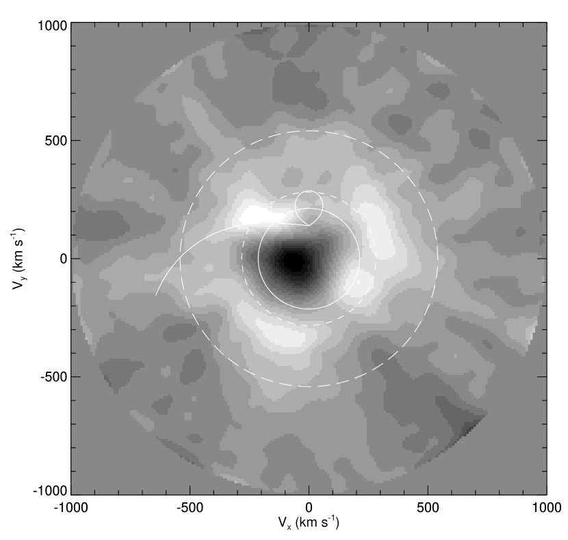
Figure 7: A velocity tomogram reconstructed from the out-of-eclipse H$\alpha$ profiles of RY Per (after subtraction of an assumed photospheric component). The image displays the net flux in a $201\times 201$ velocity grid at increments of 10 km s^-1, and the flux is portrayed in a grayscale image ranging from $-0.0034$ (black) to $+0.0029$ (white) based upon a continuum flux of unity. The model profile derived from this image corresponds to a projection through the image from a given orientation (from the top for orbital phase 0.00, from the right for phase 0.25, from the bottom for phase 0.50, and from the left for phase 0.75). The various white lines correspond to the velocity locations of binary components discussed in the text.

We show in Figure 7 this kind of Doppler tomogram for the H$\alpha$ observations of RY Per. This image was made by subtracting the photospheric profile shown in Figure 6 from the secondary subtracted H$\alpha$ profiles for out-of-eclipse orbital phases (Fig. 3), and then performing a back projection tomographic reconstruction using the algorithm described by Thaller et al. (2001). The resulting tomogram is shown in the velocity reference frame of the primary star where $V_{x}$ is the velocity component along the axis from the primary to the secondary and $V_{y}$ is the orthogonal velocity component in the orbital plane in the direction of orbital motion. The model line profile corresponding to the tomogram is calculated by a projection through this image from a particular orientation (for example, the profile for phase 0.00 is a projection from the top of the figure to the bottom, while that for phase 0.25 is from the right to the left hand side). We also show in Figure 7 the velocity locations of the principal components in the binary that could influence the distribution of circumstellar gas. The large solid-line circle indicates the velocity limits of the projected rotational velocity of the primary while the smaller solid-line figure shows the velocity limits of the Roche-filling secondary (made assuming synchronous rotation of the secondary). The solid-line arc originating at the inner L1 point shows the velocity trajectory of a ballistic gas stream which is terminated where the stream impacts the primary (Lubow & Shu, 1975). The outer long-dashed circle shows the location of disk Keplerian motion at the primary’s surface while the inner short-dashed circle shows the Keplerian motion at the outer disk edge (corresponding to the Roche limit of the primary).

The tomogram image in Figure 7 presents a number of problems that challenge the assumptions underlying its calculation. The image is dominated by a dark central absorption that actually reaches a minimum flux value below zero (in conflict with the premise that the profile is the result of a sum of flux emitting elements). This results from the fact that at the high inclination of the RY Per system part of the disk appears projected against the photosphere of the primary and causes absorption of the photospheric flux. The absorption properties of the disk are ignored in a straight forward application of tomography. The tomogram image appears to indicate that most of the emission originates at velocities associated with the outer disk, but this conflicts with our result from §6 that indicated a disk density concentration peaked towards the inner part of the disk. This discrepancy is partially due to the optically thick nature of the emission in the inner disk where the total flux is set by the area of emitting surface and the assumed source function (and is insensitive to the actual density). The occultation of the disk by the primary star will be especially important for flux contributions from the inner disk (for example, we see only half the flux from the innermost disk radius at any instant), but this occultation of the disk by the star is also neglected in simple tomography. This is not a significant issue for the application of tomography to studies of cataclysmic variables where the central white dwarf is small compared to the disk dimensions, but it is important in Algol binaries like RY Per where the disk and star sizes are comparable.

Given the difficulties in interpreting a simple tomogram of the H$\alpha$ emission profiles, we decided to develop a new method to investigate the distribution of circumstellar gas in RY Per. Our approach uses the analytical line formation method outlined in §6, which accounts for geometrical occultation and optical depth effects, together with a correction scheme based upon revisions to the assumed disk surface density distribution, $\Sigma$ (see Vrielmann et al. (1999)). The goal of the algorithm is to compute the surface density of the disk over a grid of radial and azimuthal elements based upon the observed profiles over the radial velocity range from $-1000$ to $+1000$ km s^-1 in all 49 of our spectra. A coarser grid of 11 radial and 60 azimuthal zones was used to describe the disk in the calculation. We begin by setting $\Sigma$ in each zone to the best-fit value determined from our $j=0.5$ and $m=5.5$ axisymmetric disk model from §6. We then consider how a change in surface density affects the flux from a given disk element,

$${{dF_{\lambda}}\over{d\Sigma}}=A~{}(S^{L}-P_{\lambda})~{}e^{-\tau_{\lambda}}~{}{{\tau_{\lambda}}\over\Sigma}.$$ (9)

In optically thin emitting elements this derivative will only be significantly different from zero close to the wavelength corresponding to the Doppler shift of the disk element. On the other hand, in optically thick elements the derivative is small near line center and significant flux increases can only occur in the “damping” wings of the profile where $\tau_{\lambda}\approx 1$. Thus, to correct the surface density of a specific disk element we need to compare the observed spectrum $O_{\lambda}$ with our current calculated spectrum $C_{\lambda}$ at those few wavelengths where the absolute value of the derivative attains a maximum. We selected only those wavelength points where the absolute value of the derivative is greater than $90\%$ of its maximum value. Such wavelength points are assigned a weight $W_{\lambda}=1$ while all the other wavelength points have $W_{\lambda}=0$. We then made the simple assumption that the observed deviation can be attributed entirely to a surface density correction at that particular element,

$${{\triangle\Sigma}\over\Sigma}=\int{{\gamma~{}(O_{\lambda}-C_{\lambda})}\over{A~{}(S^{L}-P_{\lambda})~{}e^{-\tau_{\lambda}}~{}\tau_{\lambda}}}~{}W_{\lambda}~{}d\lambda~{}/~{}\int W_{\lambda}~{}d\lambda.$$ (10)

In fact there may be many disk elements that have the correct Doppler shift to also contribute to the correction $O_{\lambda}-C_{\lambda}$ at any specific wavelength, so we introduce a gain factor $\gamma$ that is close to zero to make the corrections slowly and iteratively. The algorithm progresses through each spectrum available and determines a surface density correction if the element is visible at that orbital phase (i.e., free of occultation by the primary and secondary). Then a mean correction is found from the average of all the available spectra and the surface density is revised accordingly. Since large deviations in $\Sigma$ between neighboring disk elements are unphysical, we perform a boxcar smoothing in $\log\Sigma$ over 3 adjacent elements at this stage. The entire algorithm is then iterated to find new corrections until the root mean square of the whole set of $O_{\lambda}-C_{\lambda}$ differences reaches a minimum.

We performed a number of tests to determine how well the algorithm could reconstruct an arbitrarily defined disk surface distribution using a set of model spectra with the same orbital phase distribution and instrumental broadening as our observed set. We found that disk azimuthal perturbations of the form $\cos n\phi$ where $n<4$ were successfully reconstructed with a typical deviation of $\approx 10\%$ from the predefined density over most of the disk. We also performed tests where the radial density distribution was altered in the inner and/or outer portions of the disk. These were also successful except in the inner optically thick regions where the reconstructed surface densities never departed significantly from their initial default values. This is due to the fact that flux from such optically thick elements is relatively insensitive to the density. We also found that model density distributions with small regions of differing density (either enhanced or reduced) were not reconstructed correctly if the affected surface area was less than $10\%$ of the total disk area (such density perturbations appear broader and have lower contrast in the reconstructions). This stems from the fact that many elements can contribute to a flux correction at a given wavelength since many elements share a similar radial velocity, and consequently any small deviation seen in the profiles tends to be redistributed over many area elements in this kind of reconstruction. Thus, we believe the algorithm can succeed in reconstructing large scale disk features, but we cannot rely upon it to reproduce fine structure or to find accurate density perturbations in optically thick zones.

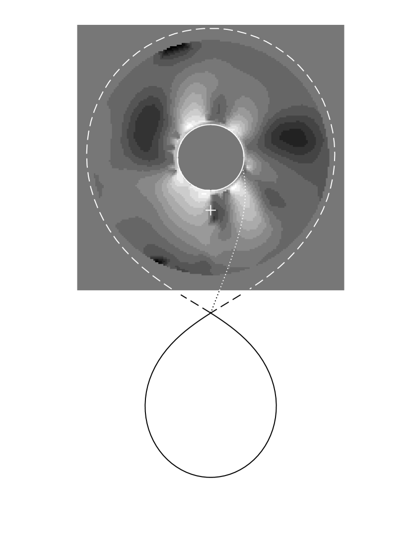
Figure 8: A 16 level grayscale depiction of the logarithm of the disk surface density in a spatial diagram as viewed from above the orbital plane. The Roche-filling secondary is shown in outline on the right while the primary star is located at the center of the disk. The dashed line indicates the Roche limit of the primary, and the dotted line shows the ballistic trajectory of the gas stream from the secondary star.

We show in Figure 8 the resulting surface density map (in a logarithmic scaling) based upon all of the observed H$\alpha$ profiles. The calculation was made with 9 iterations and a gain $\gamma=0.02$. The spatial dimensions of the disk grid are shown in relation to the system components in a view from above the orbital plane, with the secondary on the right and the primary on the left in the middle of the disk image. The dashed line indicates the primary’s Roche limit in the orbital plane, and the plus sign marks the center of mass. The dotted line represents the ballistic trajectory of a gas stream originating at the inner Lagrangian point (Lubow & Shu, 1975). The disk surface density in this map appears to have a somewhat elongated distribution aligned approximately with the axis joining the stars, i.e., the surface density is lower in the directions orthogonal to this axis (in the vicinity of $\phi=90^{\circ}$ and $270^{\circ}$). Figure 9 plots the average radial decline in disk density for quadrants centered on $\phi=90^{\circ}$ and $270^{\circ}$ compared with the average for quadrants centered on $\phi=0^{\circ}$ and $180^{\circ}$. The disk density appears to be approximately $4\times$ lower in the regions orthogonal to the axis. Figure 8 also indicates that the disk may have a local density enhancement in the region where the gas stream approaches the primary.

Richards & Ratliff (1998) made hydrodynamical simulations of the gas flows of two Algol binary systems, $\beta$ Per and TT Hya. The systems differ in where the gas stream encounters the primary: the stream hits the primary in $\beta$ Per near an azimuth of $\phi\approx 60^{\circ}$ while it misses the limb of the primary altogether for TT Hya. The stream geometry in RY Per lies between these cases but we do expect that a stream – star impact occurs (Fig. 8). The best comparison can be made with their simulation for $\beta$ Per at the conclusion of a long time sequence (see Fig. 6 in Richards & Ratliff (1998)). Their results show that some of the incoming gas stream is deflected into plumes that extend in the direction of $\phi=180^{\circ}$, and some of this material passes close to the primary on a return trajectory to occupy the region around $\phi=0^{\circ}$. We suspect that the elongated surface density distribution we find for RY Per (Fig. 8) indicates that similar kinds of flows are occurring in its disk (at least in a time-averaged sense based upon results from spectra taken on many dates).

The hydrodynamical simulations of Richards & Ratliff (1998) are also important in demonstrating some of the limitations of our disk mapping techniques. Richards & Ratliff (1998) find that the gas temperature varies significantly in the circumstellar material, attaining peak values near the impact site and in diffuse regions between dense gas filaments that surround the primary (the existence of a hot disk component is supported by UV observations of highly ionized emission lines; Peters (2001)). Our model assumes an isothermal disk, so it is possible that some disk elements in our model (for example, those near the hot impact site) are assigned too low a surface density because H$\alpha$ emissivity declines with increasing temperature (Richards & Ratliff, 1998). However, the hydrodynamical simulations suggest that, with the exception of the always hot impact zone, most disk regions will experience similarly diverse temperature fluctuations, so that a time-averaged map like ours should not be too adversely affected by the assumption of constant temperature. The hydrodynamical simulations also show that the gas flow velocities can depart significantly from Keplerian motion, particularly in regions close to the star. Our model will suffer by assigning an incorrect velocity to certain disk elements, but since the main effect of gas close to the star is to create increased absorption of the photospheric flux where such elements are moving nearly tangentially to the line of sight, we doubt that non-Keplerian flows will seriously alter the appearance of the surface density map.

The inclusion of the disk asymmetries in our model line profiles decreases the root mean square of the $O_{\lambda}-C_{\lambda}$ residuals from 0.035 of the continuum flux in the axisymmetric case (§6) to 0.031 in the converged model. Taken at face value this is only a modest improvement, but recall that most of this difference is due to temporal variations which are probably larger than the orbital phase-related variations (Fig. 3). The simulated spectra based upon the density map in Figure 8 are shown as dashed lines in Figures 3 – 5, and on the whole these model profiles provide a better match of the observations than those based upon the axisymmetric model. This is especially true in the eclipse sequences; for example, the blue wing variations in Figure 4 are much more closely reproduced when the disk density is lower in regions orthogonal to the axis joining the stars. Thus, we conclude that the disk density structures indicated in the reconstructed map are required to model adequately the observed H$\alpha$ variations.

8 Conclusions

The H$\alpha$ observations of RY Per indicate that the mass gainer in this Algol-type binary is surrounded by a time variable accretion disk. The H$\alpha$ profile usually appears as a double-peaked emission line with a strong central absorption. This same profile morphology appears in the Be shell stars, and we fit the mean H$\alpha$ profile of RY Per using the line formation method that Hummel & Vrancken (2000) have applied to Be stars. We can match the observed and model profiles if the accretion disk has a steep radial decline in surface density and experiences Keplerian motion. The calculation demonstrates the importance of accounting for disk absorption in the analysis of the emission lines. The presence of orbital phase-related variations in the H$\alpha$ profile implies that the disk is structured, and we developed a new method of tomographic reconstruction to derive a map of the disk surface density (based upon the spatial and velocity relationship for Keplerian motion). The density map shows similarities to the results of hydrodynamical simulations of gas flows in Algols (Richards & Ratliff, 1998) and suggests that the incoming gas stream is deflected at the impact site into elongated trajectories that create density enhancements along the axis joining the stars.

Our interest in RY Per was sparked by its rapid rotation (§4) which is probably the result of the accretion of gas with high angular momentum. The dimensions of the RY Per system are such that the gas stream strikes the star very close to its trailing edge (Fig. 8), and this is clearly a favorable situation to impart angular momentum from the gas stream to the primary. Algol binaries become more widely separated as mass transfer continues (Hilditch, 2001), so that in the past when the components of RY Per were closer the gas stream would have hit the primary closer to its center, a less favorable geometry to gain angular momentum. We can calculate how the angular momentum gain varies as the system mass ratio changes by considering the angle $\psi$ between the surface normal and the gas stream velocity vector $\vec{V}$ at the point of impact.

Figure 10 shows a sample calculation of the magnitude of $\vec{V}\times\vec{R}=VR\sin\psi$ based upon a conservative mass transfer evolutionary path for RY Per. We constructed a series of gas stream trajectories for a grid of mass ratios $q=M_{S}/M_{P}$ (Lubow & Shu, 1975). In each case the system semi-major axis was computed according to

$${a\over{a_{1}}}={1\over{16}}~{}{{(1+q)^{4}}\over{q^{2}}}$$ (11)

where $a_{1}$ was the closest separation at the time when the stars had the same mass ($q=1$). The radius of the mass gainer was estimated from its mass according to the mass – radius relation for main sequence stars, $R\propto M^{0.64}$. The point of impact and the value of $\vec{V}\times\vec{R}$ were derived for each test value of $q$. We found that for mass ratios $q<0.22$ the stream missed the star altogether. We assume in these cases that the gas will end up in an accretion disk and will eventually reach the stellar surface with the Keplerian velocity. Figure 10 shows that as the system evolves to lower values of $q$ the mass gainer receives more and more angular momentum per gram of gas accreted. It is interesting to note that the current position of RY Per in this diagram (indicated by the solid dot) is near the peak of the angular momentum transfer efficiency.

The angular momentum efficiency variation suggests that the spin up of the mass gainer may become more pronounced as systems approach the peak of the efficiency curve. Other factors such as the mass transfer rate and tidal and magnetic breaking will also play important roles in the effective spin up of the gainer star. Nevertheless, it is worthwhile considering whether other systems like RY Per also show evidence of spin up when they reach the efficiency maximum. Figure 11 shows the location of RY Per (solid circle) in the $r-q$ diagram in which the fractional radius of the gainer is plotted against the system mass ratio. The solid line shows the evolutionary path followed by RY Per as the system evolves from large to small $q$ and the semimajor axis increases. The dotted curve labelled by $\bar{\omega}_{\rm min}$ shows the minimum distance between the gas stream and center of the gainer (Lubow & Shu, 1975), and once the gainer’s radius is smaller than this value the gas stream will miss the star and form a disk (the intersection of the curves corresponds to the discontinuity in Fig. 10). Algol binaries found below $\bar{\omega}_{\rm min}$ generally have well developed, permanent accretion disks (Peters, 2001). The dashed curve marked by $\bar{\omega}_{\rm d}$ is the fractional outer radius of a disk in which the orbital velocity at the stream – disk intersection matches the vector component of the stream in the same direction (Lubow & Shu, 1975). Most dense accretion disks can form only if the stellar radius is smaller than $\bar{\omega}_{\rm d}$, and Algols above this line show no evidence of disks (Peters, 2001). RY Per falls in the region between the curves, and other systems in this same region have variable disks (Peters, 2001).

We also show in Figure 11 the positions of gainers in 34 other Algol binaries from the study of Van Hamme & Wilson (1990) (see their Table 6). Van Hamme & Wilson (1990) list the ratio of primary’s angular spin velocity to the orbital angular velocity, and the open circular area plotted for each system in Figure 11 is proportional to this ratio (rapid rotators have larger symbols). There appears to be a trend for the rapid rotators to appear in the lower left portion of this diagram, which corresponds to the evolutionary stage near the peak of the angular momentum transfer efficiency (Fig. 10). This suggests that gainers in most Algols are significantly spun up once they reach the stage where the gas stream strikes the star nearly tangentially (the epoch in which we now find RY Per).

The example of RY Per demonstrates clearly how massive stars can be spun by mass transfer in close binaries. Such systems will increase their separation as mass transfer progresses making it more and more difficult for tidal forces to slow the rotation of the gainer, and consequently the gainer may remain a rapid rotator for most of its main sequence lifetime (barring further interaction with the secondary). Since many stars are members of close binaries, these mass and angular momentum transfer processes could plausibly account for a significant fraction of the population of rapidly rotating massive stars (Pols et al., 1991; Van Bever & Vanbeveren, 1997; Gies, 2001).

Table 1: KPNO Coude Feed Observing Runs

UT Dates	G/$\lambda_{b}$/O	Filter	$\lambda/\Delta\lambda$	Range (Å)
1999 Oct 12 – 18	316/ 7500/1	GG495	4100	5400 – 6736
1999 Nov 09 – 15	316/ 7500/1	GG495	4400	5545 – 6881
1999 Dec 04 – 09	632/12000/2	OG550	31000	6456 – 6774
2000 Oct 02 – 04	316/12000/2	OG550	9500	6440 – 7105

Table 2: Radial Velocities for the Secondary

HJD	Spectroscopic	$V_{r}$	$O-C$
(2,400,000$+$)	Phase	(km s-1)	(km s-1)
51463.715	0.526	0$-23.1$	0+$0.3$
51463.737	0.529	0$-17.0$	0+$3.1$
51463.761	0.533	0$-15.5$	0+$1.0$
51463.783	0.536	0$-12.1$	0+$1.2$
51463.804	0.539	00$-9.4$	0+$0.8$
51463.828	0.543	00$-4.6$	0+$1.9$
51463.850	0.546	00$-2.0$	0+$1.3$
51463.871	0.549	00$-1.8$	0$-1.6$
51463.895	0.552	00+$3.3$	0$-0.2$
51463.916	0.555	00+$4.9$	0$-1.7$
51463.937	0.558	0+$10.6$	0+$0.8$
51463.960	0.562	0+$14.0$	0+$0.8$
51463.992	0.566	0+$16.8$	0$-1.1$
51464.874	0.695	+$132.4$	0+$0.5$
51465.732	0.820	+$168.9$	0$-0.1$
51465.982	0.856	+$155.2$	0$-4.4$
51466.722	0.964	0+$81.8$	0+$2.1$
51466.953	0.998	0+$41.5$	0$-1.7$
51466.975	0.001	0+$37.7$	0$-1.9$
51467.745	0.113	0$-90.6$	0$-2.9$
51467.766	0.116	0$-87.7$	0+$3.1$
51467.945	0.142	$-111.2$	0+$4.3$
51467.966	0.145	$-114.9$	0+$3.2$
51468.730	0.257	$-180.8$	0$-3.8$
51468.909	0.283	$-181.7$	0$-2.8$
51468.930	0.286	$-180.4$	0$-1.7$
51469.739	0.404	$-128.8$	0+$4.0$
51469.760	0.407	$-123.3$	0+$7.3$
51469.941	0.433	$-104.3$	0+$6.2$
51491.858	0.626	0+$73.7$	0$-3.0$
51492.802	0.764	+$166.2$	0+$1.3$
51493.798	0.909	+$130.3$	0+$0.9$
51494.808	0.056	0$-27.1$	0$-2.2$
51494.830	0.059	0$-29.9$	0$-1.4$
51495.852	0.208	$-161.7$	0$-0.4$
51496.844	0.353	$-172.0$	0$-9.8$
51497.811	0.494	0$-56.8$	0$-1.2$
51516.669	0.241	$-170.5$	0+$3.1$
51517.664	0.386	$-143.3$	0+$0.9$
51521.681	0.971	0+$74.1$	0+$2.0$
51819.777	0.403	$-134.9$	0$-1.7$
51820.677	0.534	0$-15.0$	0$-0.1$
51820.714	0.540	00$-9.2$	0+$0.3$
51820.763	0.547	00$-4.2$	0$-2.1$
51820.806	0.553	00+$3.8$	0$-0.4$
51820.852	0.560	0+$11.3$	0+$0.2$
51820.896	0.566	0+$12.8$	0$-4.9$
51820.962	0.576	0+$20.2$	0$-7.2$
51821.842	0.704	+$145.2$	0+$7.4$

Table 3: Radial Velocities for the Primary

HJD	Spectroscopic	$V_{r}$	$O-C$
(2,400,000$+$)	Phase	(km s-1)	(km s-1)
48155.075	0.441	0+$40.8$	0+$0.4$
49650.939	0.383	0+$55.8$	0+$3.9$
49652.926	0.672	0$-30.3$	$-11.0$
49653.947	0.821	0$-31.5$	0+$2.1$
49654.935	0.965	00+$1.5$	+$10.5$
49655.941	0.112	0+$25.8$	0$-9.9$
49656.967	0.261	0+$56.6$	0$-3.8$
49659.690	0.658	0$-16.0$	0+$0.1$
49671.873	0.433	0+$49.8$	0+$7.6$

Table 4: Orbital Elements

Element	Popper (1989)	This Work
$P$ (d)	6.863569	6.863569
$T_{P}$ (HJD – 2,400,000)	$\cdots$	$51467.15\pm 0.10$
$T_{S}$ (HJD – 2,400,000)	$\cdots$	$51466.97\pm 0.13$
$e$	0.0	$0.036\pm 0.005$
$\omega_{P}$ (deg)	$\cdots$	255
$\omega_{S}$ (deg)	$\cdots$	$75\pm 7$
$K_{P}$ (km s-1)	$50.1\pm 2.1$	$47.3\pm 3.9$
$K_{S}$ (km s-1)	$175.8\pm 1.2$	$174.5\pm 0.9$
$V_{P}$ (km s-1)	$-11.6\pm 1.5$	$13.8\pm 2.9$
$V_{S}$ (km s-1)	$-6\pm 2$	$-6.0\pm 0.6$
rmsP (km s-1)	8.8	8.4
rmsS (km s-1)	5.7	3.4
$M_{P}$ ($M_{\odot}$)	$\cdots$	$6.24\pm 0.24$
$M_{S}$ ($M_{\odot}$)	$\cdots$	$1.69\pm 0.23$
$a$ ($R_{\odot}$)	$\cdots$	$30.3\pm 0.6$

Figure 1: The fitted radial velocity curves (solid lines) for RY Per together with the observed data for the secondary (open circles) and the primary star (filled circles). Phase 0.0 corresponds to periastron.

Figure 2: Tomographically reconstructed spectra of the primary (bottom) and secondary (middle) based upon outside-of-eclipse spectra and rectified to a unit continuum. The upper plot shows a single spectrum obtained at mid-eclipse when the flux is entirely due to the secondary (except for disk emission at H$\alpha$).

Figure 3: Secondary subtracted H$\alpha$ profiles for the out-of-eclipse sample. The spectra are plotted in the velocity frame of the primary star. Each spectrum is aligned so that the continuum level is set at the orbital phase of observation (phase 0.0 corresponds to primary eclipse). The bar at the upper right gives the spectral intensity scale relative to a primary continuum flux of unity. The dashed lines represent model spectra derived from the reconstruction of the disk surface density (§7).

Figure 4: Secondary subtracted H$\alpha$ profiles for the eclipse observed on 1999 October 12 (in a format similar to Fig. 3). The dotted lines show model predictions for eclipses of an axisymmetric disk (§6), and these are extended before and after the observed sequence to show the predicted behavior beyond the times of mid-eclipse. The dashed lines represent model spectra derived from the reconstruction of the disk surface density (§7).

Figure 5: Secondary subtracted H$\alpha$ profiles for the eclipse observed on 2000 October 03 (in the same format as Fig. 4).

Figure 6: The tomographically reconstructed H$\alpha$ profile of the primary star (plus signs) together with several axisymmetric disk model profiles: $j=0.5$, $m=5.5$ (solid line); $j=0.5$, $m=2$ (dashed line); $j=1$, $m=6$ (dotted line). Also shown is the model rotationally broadened absorption profile for the photosphere of the primary (dot-dashed line).

Figure 9: The logarithm (base 10) of the surface density as a function of radial distance in the disk based upon the axisymmetric model (solid line). The radial dependence is also shown for the reconstructed surface density map for the average of two quadrants centered on the axis ($\phi=0^{\circ}$ and $180^{\circ}$, dotted line) and the average of two quadrants orthogonal to the axis (centered on $\phi=90^{\circ}$ and $270^{\circ}$, dashed line).

Figure 10: The evolution of angular momentum transfer efficiency for a conservative mass transfer scenario for RY Per. The curve shows the amplitude of $\vec{V}\times\vec{R}$, the vector component of angular momentum from the gas stream at the point of impact, as function of $q=M_{S}/M_{P}$ (which decreases with time). The solid dot shows the current state of RY Per. The discontinuity near $q=0.2$ marks the boundary where the gas stream misses the star and angular momentum is accreted according to the Keplerian velocity at the stellar surface.

Figure 11: An $r,q$ diagram showing the location of the mass gainers in RY Per (solid circle) and other Algol binaries (Van Hamme & Wilson, 1990) (open circles). The area of each circle is proportional to the ratio of the gainer’s angular velocity compared to the synchronous rate. The solid line shows the evolutionary path of RY Per for conservative mass transfer. The dotted curve labelled by $\bar{\omega}_{\rm min}$ shows the minimum distance between the gas stream and center of the gainer, and the dashed curve marked by $\bar{\omega}_{\rm d}$ is the fractional outer radius of a disk in which the orbital velocity at the stream – disk intersection matches the vector component of the stream in the same direction (Lubow & Shu, 1975).

References

- Abt et al. (2002) Abt, H. A., Levato, H., & Grosso, M. 2002, ApJ, 573, 359
- Abt & Levy (1978) Abt, H. A., & Levy, S. G. 1978, ApJS, 36, 241
- Bagnuolo et al. (1994) Bagnuolo, W. G., Jr., Gies, D. R., Hahula, M. E., Wiemker, R., & Wiggs, M. S. 1994, ApJ, 423, 446
- Barbier-Brossat & Figon (2000) Barbier-Brossat, M., & Figon, P. 2000, A&AS, 142, 217
- Donnison & Mikulskis (1995) Donnison, J. R., & Mikulskis, D. F. 1995, MNRAS, 272, 1
- Etzel & Olson (1993) Etzel, P. B., & Olson, E. C. 1993, AJ, 106, 1200
- Gies (2001) Gies, D. R. 2001, in The influence of binaries on stellar population studies (ASSL Vol. 264), ed. D. Vanbeveren (Dordrecht: Kluwer), 95
- Gies et al. (1998) Gies, D. R., Bagnuolo, W. G., Jr., Ferrara, E. C., Kaye, A. B., Thaller, M. L., Penny, L. R., & Peters, G. J. 1998, ApJ, 493, 440
- Gies et al. (2002) Gies, D. R., Penny, L. R., Mayer, P. Drechsel, H., & Lorenz, R. 2002, ApJ, 574, 957
- Gray (1992) Gray, D. F. 1992, The Observation and Analysis of Stellar Photospheres, 2nd ed. (Cambridge: Cambridge Univ. Press)
- Harvin et al. (2002) Harvin, J. A., Gies, D. R., Bagnuolo, W. G., Jr., Penny, L. R., & Thaller, M. L. 2002, ApJ, 565, 1216
- Hilditch (2001) Hilditch, R. W. 2001, An Introduction to Close Binary Stars (Cambridge: Cambridge Univ. Press)
- Hill et al. (1971) Hill, G., Barnes, J. V., Hutchings, J. B., & Pearce, J. A. 1971, ApJ, 168, 443
- Horne (1995) Horne, K. 1995, A&A, 297, 273
- Horne & Marsh (1986) Horne, K., & Marsh, T. R. 1986, MNRAS, 218, 761
- Howarth et al. (1997) Howarth, I. D., Siebert, K. W., Hussain, G. A. J., & Prinja, R. K. 1997, MNRAS, 284, 265
- Hummel & Vrancken (2000) Hummel, W., & Vrancken, M. 2000, A&A, 359, 1075
- Kreiner et al. (2001) Kreiner, J. M., Kim, C., & Nha, I. 2001, An Atlas of Diagrams of Eclipsing Binary Stars (Cracow, Poland: Wydawnictwo Naukowe Akademii Pedagogicznej)
- Kurucz (1994) Kurucz, R. L. 1994, Solar Abundance Model Atmospheres for 0, 1, 2, 4, 8 km/s, Kurucz CD-ROM No. 19 (Cambridge, MA: Smithsonian Astrophysical Obs.)
- Lanz & Hubeny (2003) Lanz, T., & Hubeny, I. 2003, ApJS, 146, 417
- Lubow & Shu (1975) Lubow, S. H., & Shu, F. H. 1975, ApJ, 198, 383
- Lucy & Sweeney (1971) Lucy, L. B., & Sweeney, M. A. 1971, AJ, 76, 544
- Morbey & Brosterhus (1974) Morbey, C. L., & Brosterhus, E. B. 1974, PASP, 86, 455
- Olson & Plavec (1997) Olson, E. C., & Plavec, M. J. 1997, AJ, 113, 425
- Penny et al. (2002) Penny, L. R., Gies, D. R., Wise, J. H., Stickland, D. J., & Lloyd, C. 2002, ApJ, 575, 1050
- Peters (1989) Peters, G. J. 1989, Sp. Sci. Rev., 50, 9
- Peters (2001) Peters, G. J. 2001, in The influence of binaries on stellar population studies (ASSL Vol. 264), ed. D. Vanbeveren (Dordrecht: Kluwer), 79
- Pols et al. (1991) Pols, O. R., Coté, J., Waters, L. B. F. M., & Heise, J. 1991, A&A, 241, 419
- Popper (1989) Popper, D. M. 1989, ApJS, 71, 595
- Popper & Dumont (1977) Popper, D. M., & Dumont, P. J. 1977, AJ, 82, 216
- Richards (2001) Richards, M. T. 2001, in Astrotomography, Indirect Imaging Methods in Observational Astronomy, Lecture Notes in Physics 573, ed. H. M. J. Boffin, D. Steeghs, & J. Cuypers (Berlin, Heidelberg: Springer-Verlag), 276