Simulation of stellar instabilities with vastly different timescales using domain decomposition

Abstract

Strange mode instabilities in the envelopes of massive stars lead to shock waves, which can oscillate on a much shorter timescale than that associated with the primary instability. The phenomenon is studied by direct numerical simulation using a, with respect to time, implicit Lagrangian scheme, which allows for the variation by several orders of magnitude of the dependent variables. The timestep for the simulation of the system is reduced appreciably by the shock oscillations and prevents its long term study. A procedure based on domain decomposition is proposed to surmount the difficulty of vastly different timescales in various regions of the stellar envelope and thus to enable the desired long term simulations. Criteria for domain decomposition are derived and the proper treatment of the resulting inner boundaries is discussed. Tests of the approach are presented and its viability is demonstrated by application to a model for the star P Cygni. In this investigation primarily the feasibility of domain decomposition for the problem considered is studied. We intend to use the results as the basis of an extension to two dimensional simulations.

1 INTRODUCTION

Sufficiently luminous objects, such as massive stars, are known to suffer from strange mode instabilities with growth rates in the dynamical range (Kiriakidis, Fricke & Glatzel, 1993; Glatzel & Kiriakidis, 1993). The boundary of the domain in the Hertzsprung-Russel diagram (HRD) above which all stellar models are unstable - irrespective of their metallicity -, coincides with the observed Humphreys-Davidson (HD) limit (Humphreys R.M. & Davidson K., 1979). Moreover, the range of unstable models covers the stellar parameters for which the LBV (luminous blue variable) phenomenon is observed (for a review see Humphreys R.M. & Davidson K. (1994)).

The high growth rates of the instabilities indicate a connection to the observed mass loss of the corresponding objects. To verify this suggestion, simulations of their evolution into the non linear regime have been performed. In fact, for selected models Glatzel, Kiriakidis, Chernigovskij & Fricke (1999) found the velocity amplitude to exceed the escape velocity (see, however, Dorfi & Gautschy (2000)).

To identify a possible connection between non linear pulsations and outbursts in luminous blue variables Grott, Glatzel & Chernigovski (2002) have studied the evolution of an initial model located in the HRD well above the HD limit. In this study, the shocks formed in the non linear regime are captured by the H-ionization zone after a few pulsation periods. These captured shocks start to oscillate rapidly with periods of the order of the sound travel time across the H-ionisation zone, while its mean position changes on the dynamical timescale of the primary, strange mode instability. Grott, Glatzel & Chernigovski (2002) have shown, that this shock front oscillation is of physical origin and therefore must not be disregarded. In particular, the phenomenon should not be eliminated by increasing the artificial viscosity. We note that the representation of the phenomenon requires the correct treatment of extreme gradients of the dependent variables, implying their variation by several orders of magnitude. It is achieved by use of a, with respect to time implicit Lagrangian scheme.

The rapid shock oscillations, which are confined to a narrow region in the vicinity of the shock front, require an inhibitively small timestep and thus prevent long term simulations. In the present paper we propose an approach based on domain decomposition to surmount the difficulty of vastly different timescales in various regions of the stellar envelope and thus to enable the desired long term simulations. In this procedure the various domains within the envelope are to be treated separately and according to their intrinsic timescales. We expect this decomposition to speed up the calculations considerably. An even higher speedup will be achieved when applying domain decomposition to two dimensional simulations. In this sense, the present investigation may be regarded as a preliminary study for decomposition in two dimensions.

The basic equations and assumptions are introduced in Section 2. The domain decomposition approach is discussed in detail in Section 3, including a derivation of criteria for domain decomposition and an investigation of the proper treatment of the resulting inner boundaries. Moreover, tests of the approach are presented there. Its viability is demonstrated by application to a model of the star P Cygni in section 4. Our conclusions follow.

2 BASIC EQUATIONS AND ASSUMPTIONS

The evolution of instabilities of a stellar envelope is followed into the non-linear regime assuming spherical symmetry and adopting a Lagrangian description, i.e. the independent variables are the time t and the mass $M_{r}$ inside a sphere of radius $r$. The equations to be solved (see, e.g., Cox (1980)) are given by mass conservation,

$$\frac{\partial r^{3}}{\partial M_{r}}-\frac{3}{4\pi\rho} = 0$$ (1)

momentum conservation,

$$\frac{\partial^{2}r}{\partial t^{2}}+4\pi r^{2}\frac{\partial p}{\partial M_{r}}+\frac{GM_{r}}{r^{2}} = 0$$ (2)

energy conservation,

$$\frac{\partial L}{\partial M_{r}}-\epsilon-\frac{p}{\rho^{2}}\frac{\partial\rho}{\partial t}+\frac{\partial E}{\partial t} = 0$$ (3)

and the diffusion equation for energy transport,

$$\frac{\partial T}{\partial M_{r}}-\frac{3\kappa(L-L_{conv})}{64\pi^{2}acr^{4}T^{3}} = 0$$ (4)

where $\rho$, $p$, $T$, $L$, and $E$ denote density, pressure, temperature, luminosity and specific internal energy, respectively. $a$ is the Stefan-Boltzmann constant, $G$ the gravitational constant and $c$ the speed of light. We emphasise that $\partial\over\partial t$ is the substantial time derivative. For the opacities $\kappa$, the latest versions of the OPAL tables (Iglesias, Rogers & Wilson, 1992; Rogers & Iglesias, 1992) have been used. Convection is treated in the standard frozen in approximation (see Baker & Kippenhahn (1965)), i.e. the convective luminostity $L_{conv}$ is kept constant and equal to the luminosity of the hydrostatic initial model. Since the instabilities are localized in the outer envelope, the evolution of the core can be neglected. Its properties are taken into account by imposing time independent boundary conditions (e.g. by prescribing luminosity, [vanishing] velocity $v$ and [constant] radius) at the bottom of the envelope. For the envelope model, the nuclear energy generation rate $\epsilon$ vanishes. At the outer boundary, the gradient of heat sources is required to vanish ($F$ is the heat flux):

$${\rm{grad}}({\rm{div}}F)=0$$ (5)

This boundary condition implies (by using equations 1,3 and 4) boundary values for the temperature $T$ and pressure $p$. It is chosen to ensure that outgoing shocks pass through the boundary without reflection. The set of boundary conditions prescribing values for the velocity and luminosity at the bottom and values for the pressure and temperature at the top of the envelope will be denoted by $(v,L)(p,T)$ in the following.

The numerical code relies on a Lagrangian, with respect to time implicit, fully conservative difference scheme proposed by Fraley (1968) and Samarskii & Popov (1969). As a consistent extension the two dimensional version of the code currently under development (also implicit and Lagrangian) is based on the method of support operators originally suggested by Samarskii et. al. (1981) and Ardelyan & Gushchin (1982). For a thorough description of the method of support operators we refer to Shashkov (1996). To handle shock waves, artificial viscosity is used. Concerning tests of the code, we adopted the same criteria as Glatzel, Kiriakidis, Chernigovskij & Fricke (1999). We emphasise, that conservativity of the numerical scheme is of fundamental importance when simulating instabilities in a stellar envelope. Considering the distribution of internal, gravitational and kinetic energy we find, that the kinetic energy can be smaller than, e.g., the gravitational energy by several orders of magnitude. Appropriate simulations of stellar instabilities require the correct representation of the kinetic energy, and therefore energy conservation with high accuracy is indispensable. The difference scheme adopted here guarantees energy conservation.

3 DOMAIN DECOMPOSITION

3.1 Motivation for domain decomposition

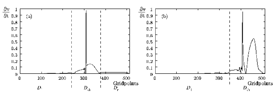
Figure 1: Normalized time derivatives of the velocity $v$ as a function of gridpoint, for two typical states of the system. Decomposition into three (a) and two (b) subdomains ($\mathcal{D}_{l}$, $\mathcal{D}_{sh}$, $\mathcal{D}_{r}$) as indicated by the dashed lines is suggested.

The stellar envelope model representing a massive star with mass $M=50M_{\odot}$, effective temperature $T_{\rm{eff}}=10^{4}K$ and luminosity $L=1.17\cdot 10^{6}L_{\odot}$, which was considered by Grott, Glatzel & Chernigovski (2002), suffers from strange-mode-instabilities. These cause pulsations with velocity amplitudes of 0.5 $v_{\rm{esc}}$ and inflate the envelope to $2.5$ initial radii. After several pulsation periods a shock front is captured in the H-ionization zone. The latter is prone to secondary instabilities and oscillates on very short timescales connected to the sound travel time across the front. These instabilities are caused by the stratification, but not driven by buoyancy (Grott, Glatzel & Chernigovski, 2002). Resolving the rapid oscillations of the shock front reduces the timestep to very small values. This is computationally extremely expensive and effectively inhibits the desired long term study of the system.

In order to enable the treatment of the problem the integration interval is decomposed such that the small and quickly varying shock region is integrated with small time steps and the remaining major part of the envelope is calculated using large time steps. This strategy of domain decomposition is common in computational fluid dynamics (see, e.g., Wu (1999) and Wu & Zou (2000)). For the treatment of interfaces between the various domains and the associated inner boundary conditions for purely hyperbolic systems, we refer the reader to these publications. We stress, however, some fundamental differences to the previous studies: One of them concerns the different character of the system of equations. So far, only purely hyperbolic systems have been considered, whereas we apply domain decomposition to a composite system of hyperbolic and parabolic equations. Moreover, we adopt a numerical scheme which is implicit in time. Again, this is in contrast to previous studies which use explicit schemes.

3.2 Criterion for domain decomposition

In this section a criterion for the proper choice of the boundaries of the various domains evolving on different timescales and therefore treated with different time steps will be presented. Considering the time derivatives of various physical quantities the velocity $v$ is found to vary most rapidly and therefore determines the time step.

Figure 1 shows the time derivatives of the velocity for two typical states of the system, where Figure 1.a corresponds to rapid shock oscillations around gridpoint 310. In this case, domain decomposition as indicated by the dashed lines is suggested. Figure 1.b represents a situation, in which the outer envelope is collapsing onto the shock (at gridpoint 410). Rapid variations are now also found above the shock. Accordingly, decomposition into two domains (as indicated by the dashed line) seems appropriate. Depending on the state of the system, we therefore need to split the domain of integration into two or three subdomains.

The size of the various domains is determined by comparing the time derivatives of velocity and temperature with the corresponding derivatives on the shock front. Therefore, as a first step, the position of the shock front has to be determined. For the models studied, the latter is defined by the maximum temperature gradient. The boundaries of the shock zone are then defined by the requirement, that the time derivative at their position corresponds to a given fraction $1/k$ of the time derivative at the shock. In other words, the set of gridpoints $\mathcal{D}_{sh}$ belonging to the shock zone may be characterized by

$$\mathcal{D}_{sh}=\left\{n:\left|\frac{\partial v}{\partial t}\right|_{n}>\frac{1}{k}\left|\frac{\partial v}{\partial t}\right|_{sh}\wedge\left|\frac{\partial T}{\partial t}\right|_{n}>\frac{1}{k}\left|\frac{\partial T}{\partial t}\right|_{sh}\right\}$$ (6)

where $n$ denotes the number of the gridpoint and derivatives with index $sh$ correspond to their maximum values found in the shock region. Accordingly, the zones below and above the shock are determined by

$$\mathcal{D}_{l} = \left\{n:n\leq\mbox{min}(\mathcal{D}_{sh})\right\}$$ (7)

$$\mathcal{D}_{r} = \left\{n:n\geq\mbox{max}(\mathcal{D}_{sh})\right\}.$$ (8)

The parameter $k$ corresponds to the ratio of timesteps in $\mathcal{D}_{l,r}$ and $\mathcal{D}_{sh}$, which favours large values of $k$. On the other hand, the size of $\mathcal{D}_{sh}$ increases with $k$, suggesting smaller values. Therefore optimum results will be obtained for a mean choice. For the considered model a value of $k=15$ turned out to be satisfactory. If the size of the domains $\mathcal{D}_{l}$ or $\mathcal{D}_{r}$ drops below a given value, they are considered to be part of the shock zone, and we arrive at a decomposition into two subdomains. For the model considered the whole grid consists of 512 gridpoints and the zones have a minimum size of 64 gridpoints.

After decomposition, the quickly varying region $\mathcal{D}_{sh}$ is integrated first with timesteps $\tau_{1},\tau_{2},\ldots,\tau_{n}$. Then the domains $\mathcal{D}_{l}$ and/or $\mathcal{D}_{r}$ are integrated with the timestep $\tau=\tau_{1}+\tau_{2}+\cdots+\tau_{n}$. The decomposition implies artificial boundaries and boundary conditions between the domains $\mathcal{D}_{l}$ and $\mathcal{D}_{sh}$ and $\mathcal{D}_{r}$ and $\mathcal{D}_{sh}$, respectively. An inconsistency is introduced, if in a first approach the explicit inner boundary conditions are either kept fixed, or linearly extrapolated in time. Both cases are contained in the following extrapolation presciption:

$$Y_{bound} = \alpha_{Y}\left(\frac{(Y-Y_{old})}{\tau_{old}}\cdot{\tau}^{\prime}+Y\right)+(1-\alpha_{Y})\cdot Y$$ (9)

$Y$ stands for $p$, $T$, $v$, $L$, and $\alpha_{Y}\in[0,1]$ is a free extrapolation parameter, which may be chosen independently for each variable. $Y$ refers to the current, $Y_{old}$ to the previous value of the variable. $\tau_{old}$ is the last, $\tau^{\prime}$ the current timestep. How the inconsistency may be treated will be discussed in the following sections.

Once the integration of all domains has been performed, one subsequent timestep is done without decomposition. We shall refer to it as the relaxation timestep. Relaxation prevents accumulation of residual errors.

3.3 The iteration procedure

A mathematically consistent way of integrating the different domains, which solves the problem of artificial fixed boundary conditions is the following iterative procedure:

1. The computation is started at time $t$ and $D_{l}$, $D_{sh}$ and $D_{r}$ are integrated with fixed boundary values $(v,L)_{t}$ and $(p,T)_{t}$ for each domain. The subscript $t$ denotes values at time $t$.

2. New boundary values $(v,L)_{t+\tau}$ and $(p,T)_{t+\tau}$ are obtained by integration of the adjacent domain. With these boundary values the integration 1 is repeated.

This iterative procedure implies implicit boundary conditions and sucessively eliminates the errors introduced by the artificial boundaries. 4-5 iteration cycles produce satisfactory results. However, this approach is computationally even more expensive than integrating the entire domain with small timesteps $\tau_{1},\ldots,\tau_{n}$. Concerning the present problem, it is therefore not relevant and has been applied only for comparison with other methods discussed below. However, for the corresponding two dimensional problem the computational effort might be significantly reduced by the procedure as the inversion of the most ill-conditioned matrix occurring there is an $N^{2}$-process.

3.4 Overlapping domains

Figure 2: Snapshot of the sound travel time $\tau_{\rm{cour}}$ (a) and the diffusion time $\tau_{\rm{diff}}$ (b) across a cell as a function of gridpoint.

One method to reduce the error caused by the fixed inner boundary conditions consists of using overlapping domains of computation. We emphasise that the system considered here is composed of hyperbolic and parabolic differential equations. We first consider the hyperbolic part, i.e., the mechanical equations. Any errors or perturbations in this part produced at the boundaries of the domains propagate with finite speed into the domain of computation along the characteristics of the equation. For our set of equations, perturbations propagate with velocities $v\pm c_{s}$, where $c_{s}$ denotes the speed of sound. If the domains overlap such that the time for error propagation across the overlap is larger than the integration timestep $\tau$, we may discard the flawed values close to the boundary and keep only the correct values for the subsequent timestep. This condition implies

$$\tau<\sum_{i}\frac{l_{i}}{v_{i}+c_{s_{i}}}$$ (10)

where the sum of individual sound travel times is to be taken over all overlapping cells. $l_{i}$ denotes the thickness of cell $i$.

Concerning the parabolic part of equations 1-4, i.e. the diffusion equation for energy transport, perturbations travel across the grid with infinite speed. Therefore, the procedure suggested for the hyperbolic part of the equations can in principle not be carried over to the parabolic part. Rather physical quantities change on the diffusion timescale, which is given by $\tau_{\rm{diff}}=l^{2}\rho c_{p}\frac{3\kappa\rho}{4acT^{3}}$ ($c_{p}$ is the specific heat at constant pressure). Consequently, we expect the effect of the perturbations to be small far from the boundary if the timestep $\tau$ is sufficiently small, i.e. :

$$\tau<\sum_{i}l_{i}^{2}\rho_{i}c_{p_{i}}\frac{3\kappa_{i}\rho_{i}}{4acT_{i}^{3}}$$ (11)

where the sum of individual diffusion times again extends over all overlapping cells.

In Figure 2 a snapshot of the sound travel time (Figure 2.a) and diffusion time (Figure 2.b) across a cell is given as a function of gridpoint. The sound travel time across the overlapping region is larger than a typical timestep (approximately 1 per cent of the global free fall time) for an overlap of $\sim 8$ cells (condition 10). However, while the diffusion time across the overlapping region is bigger than the timestep even for a small overlap in the bottom part of the envelope, condition 11 cannot be satisfied in the outer envelope for a reasonable number of overlapping cells. The latter is due to the small heat capacity there (implying the ratio of thermal and dynamical timescales to be small) and in accordance with the validity of the non-adiabatic-reversible approximation (NAR-approximation), which has been shown for this particular stellar model by Grott, Glatzel & Chernigovski (2002). How satisfactory results may be obtained even if condition 11 is not satisfied will be discussed in the following section.

3.5 Inner boundary conditions

Figure 3: The luminosity as a function of gridpoint around the boundary between $\mathcal{D}_{l}$ and $\mathcal{D}_{sh}$ at gridpoint 264. Results obtained without decomposition are shown as solid lines. Dotted lines in the left and right columns correspond to decomposition without (1) and with (2) relaxation, respectively. $(v,L)(p,T)$ and $(v,L)(v,L)$ boundary conditions have been used in (a) and (b), respectively, the iteration procedure (4 cycles) has been applied in (c) with the $(v,L)(p,T)$ boundary condition.

On the basis of the domain decomposition procedure described above, various inner boundary conditions and their consequences will be investigated in this section. In any case, overlapping domains have been used. The tests presented here have been performed at various times with similar results. Therefore the results may be regarded to be independent of the particular state of the system. In the tests, the luminosity $L$ turned out to be the most sensitive quantity concerning the errors introduced by the inner boundaries. This is due to the fact, that in our difference scheme it is only accurate to first order. Therefore $L$ is required to be reproduced satisfactorily compared to the results of the approach without decomposition.

In Figure 3 the luminosity is given as a function of gridpoint around the boundary between $\mathcal{D}_{l}$ and $\mathcal{D}_{sh}$, which is more sensitive than the boundary between $\mathcal{D}_{sh}$ and $\mathcal{D}_{r}$ with respect to the decomposition procedure. For comparison, results obtained without decomposition are shown as solid lines. Dotted lines correspond to results with decomposition, where the left and right columns illustrate those before and after relaxation, respectively.

1. Figure 3.a shows the result obtained using the $(v,L)(p,T)$ boundary condition, i.e., velocity and luminosity were prescribed at the left, and temperature and pressure at the right boundary, respectively. This condition implies a discontinuity of the luminosity (a1) and leads to an unacceptable relative error ($\sim$ 15 per cent) after relaxation (a2).

2. Figure 3.b shows the result obtained using the $(v,L)(v,L)$ boundary condition. The latter is motivated by the discontinuity of the luminosity for the previously discussed $(v,L)(p,T)$ boundary condition. Rather than the considerable discontinuity of $L$ we expect a more tolerable discontinuity of its derivative for the $(v,L)(v,L)$ boundary condition. In fact, the results given in figure 3.b1 are satisfactory. After relaxation the relative error in the luminosity is of the order of $10^{-3}$ (figure 3.b2). However, in this case the error of $L$ directly enters the boundary conditions for the subsequent timestep and leads to an accumulation of the error at the interface. This problem can be removed partially by switching between different interfaces for subsequent timesteps. The remaining error can then spread sufficently and does not influence the further integration significantly.

3. Figure 3.c shows the result obtained using the iteration procedure described in section 3.3. After four iteration cycles it is comparable to that obtained with the $(v,L)(v,L)$ boundary condition. By performing more iteration cycles the accuracy could be improved even more. However, the iteration procedure is computationally much more expensive than the alternatives discussed and therefore of no practical use.

We thus conclude, that using the domain decomposition procedure together with overlapping domains and $(v,L)(v,L)$ boundary conditions, and switching between different interfaces, yields satisfactory results at low computational cost.

3.6 Validation of the domain decomposition procedure

Figure 4: The velocity as a function of gridpoint with (dashed line) and without (solid line) domain decomposition after $5\cdot 10^{5}$ sec (a1) and $1.1\cdot 10^{6}$ sec (b1) of simulated time. All simulations start at $t=6.47\cdot 10^{7}$ sec (after the formation of the shock front) with the same initial model. In Figures (a2) and (b2) velocities obtained with decomposition are taken $10^{4}$ sec (a2) and $5\cdot 10^{4}$ sec (b2) later than their counterparts without decomposition, respectively. This physically irrelevant phaseshift reduces the differences between the two approaches significantly. For comparison, the velocity and the density after $1.1\cdot 10^{6}$ sec of simulated time are presented as a function of relative radius in figures (b3) and (c), respectively (without decomposition).

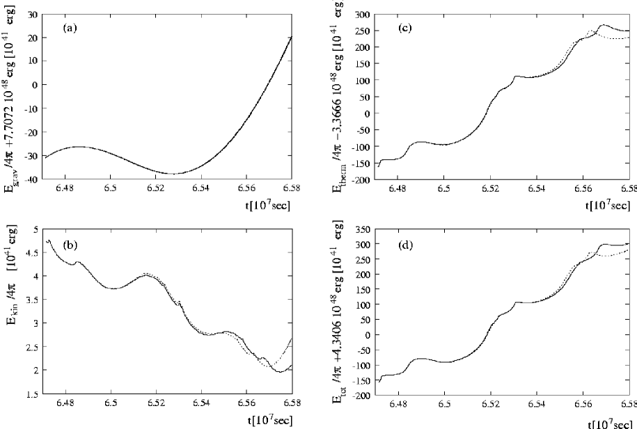
Figure 5: Gravitational (a), kinetic (b), thermal (c) and total (d) energy as a function of time. Solid and dashed lines correspond to simulations without and with domain decomposition, respectively.

The domain decomposition procedure with overlapping domains and $(v,L)(v,L)$ boundary conditions has been compared for validation with the original approach using no decomposition. The comparison starts at $6.47\cdot 10^{7}$ sec, i.e., well after the formation of the shock and the associated instability, and extends to $6.58\cdot 10^{7}$ sec. The typical periods of unstable strange modes driving the pulsations of the star are of the order of $5\cdot 10^{6}$ sec, whereas the modes carrying the stratification instabilities of the shock front have periods of $\sim 10^{5}$ sec. Therefore, the test covers approximately 0.2 periods of the overall envelope pulsations and 10 periods of shock oscillations.

Convergence and error control is done using the following criterion based on a $l^{2}$-norm:

$$\frac{1}{N}\left(\sum_{i}f_{i}^{2}\right)^{\frac{1}{2}}<E$$ (12)

where $f_{i}$ denotes the relative error of a physical quantity in gridpoint or cell $i$ and $N$ the total number of gridpoints. $E$ is the prescribed error bound and the sum extends over all gridpoints. $f_{i}^{2}$ contains the weight-function of the $l^{2}$-norm which is chosen to be proportional to the mass of the corresponding cell, $f_{i}^{2}\propto m_{i}$. Thus the various regions of the star contribute to the error in a different way and domain decomposition using the same error bound in all domains will result in different accuracies for the various domains and compared with the approach without domain decomposition. Accordingly the error bound has to be adapted to the domains contribution to the numerical error. On the other hand, as an identical error control cannot be guaranteed, results with and without decomposition are expected to differ slightly.

In the following figures 4 and 5, solid lines correspond to the approach without decompostion, dotted lines refer to decomposition. Figure 4 shows the velocity $v$ as a function of gridpoint after $5\cdot 10^{5}$ sec (figure 4.a1) and $1.1\cdot 10^{6}$ sec (figure 4.b1) of simulated time, respectively. For comparison, the velocity and the density after $1.1\cdot 10^{6}$ sec of simulated time are also presented as a function of relative radius in figures (b3) and (c), respectively (without decomposition). The shock is located at $r/R\approx 0.95$ and resolved by approximately 150 gridpoints. The high resolution of the shock zone is necessary to represent its oscillations (Grott, Glatzel & Chernigovski (2002)).

Considering $5\cdot 10^{5}$ sec of simulated time, domain decomposition yields excellent agreement with the original approach up to the position of the shock front (at grid point 320). Around the shock front the results differ slightly, whereas above it the agreement between the two approaches is again satisfying. The agreement may be found to be even better, if a phaseshift in time of about $10^{4}$ sec between the results discussed is taken into account, i.e., if results of the original approach are compared with those obtained $10^{4}$ sec later with decompostion (figure 4.a2). We emphasise, that the time interval corresponds to five oscillation cycles of the shock front instability, and implies a phaseshift of only $\frac{\pi}{5}$. With respect to the fact that the phaseshift is physically irrelevant, we thus regard the agreement as fully satisfying.

After $1.1\cdot 10^{6}$ sec of simulated time the differences become more pronounced, in particular in the vicinity of the shock (now at gridpoint 300). Similar to the previous discussion, however, including a suitable phaseshift of $5\cdot 10^{4}$ sec a reasonable agreement may be achieved (Figure 4.b2).

Figure 5 shows the gravitational (Figure 5.a), kinetic (Figure 5.b), thermal (Figure 5.c) and total energy (Figure 5.d) of the envelope as a function of time. We note that the kinetic energy given in figure 5.b is seven orders of magnitude smaller than either the gravitational or thermal energy. It may be referred to as the energy of the pulsation and is therefore of central interest in the present context. Its variation with time is one order of magnitude smaller than that of the gravitational energy, which itself is one order of magnitude smaller than that of the thermal energy. Therefore the variation of the total energy is dominated by the thermal energy.

Domain decomposition reproduces the gravitational energy perfectly. This can be attributed to the use of overlapping domains, since without them considerable disagreement is found. The latter consists of oscillations of the solution around the curve given in Figure 5.a. With respect to kinetic (Figure 5.b), thermal (5.c) and total energy (5.d), the agreement is satisfactory up to the time $6.55\cdot 10^{7}$ sec. The deviations at later times can be partially attributed to the phase shift discussed above.

To summarise, our comparisons prove the domain decomposition procedure to provide reliable and satisfactory results. We emphasise that domain decomposition violates the conservativity otherwise inherent in the numerical scheme. How this violation of conservativity contributes to the discrepancies discussed is an open question.

3.7 Speed-Up of the calculations

In order to estimate the speed-up achieved by the domain decomposition procedure, we assume that the number of iterations $I$ needed to solve the implicit equations with prescribed accuracy is not changed by decomposition, i.e., for convergence $I$ iterations are required in the shock region $\mathcal{D}_{sh}$ integrated with timestep $\tau$ and the same number of iterations $I$ are needed to integrate the domains $\mathcal{D}_{l}$ and $\mathcal{D}_{r}$ with time step $k\cdot\tau$. Moreover, we assume that $I$ iterations are required to integrate with timestep $\tau$ and without decomposition.

We denote the number of gridpoints by $N$ and the size of the domains $\mathcal{D}_{l}$, $\mathcal{D}_{sh}$ and $\mathcal{D}_{r}$ by $N_{l}$, $N_{sh}$ and $N_{r}$, respectively. ($N_{l}$, $N_{sh}$ and $N_{r}$ include the overlap.) Integrating $k$ timesteps $\tau$ without decomposition then requires

$$O_{1}=k\cdot N\cdot I$$ (13)

operations. Decomposing the grid into two or three domains, we need for the integration of the same time interval

$$O_{2} = N_{l}\cdot I+k\cdot N_{sh}\cdot I\quad\mbox{and}$$ (14)

$$O_{3} = (N_{l}+N_{r})\cdot I+k\cdot N_{sh}\cdot I$$ (15)

operations, respectively. Thus we expect a speed-up of the calculations by decomposition by a factor of

$$s_{2} = \frac{O_{1}}{O_{2}}=\frac{kN}{N_{l}+kN_{sh}}\quad\mbox{and}$$ (16)

$$s_{3} = \frac{O_{1}}{O_{3}}=\frac{kN}{(N_{l}+N_{r})+kN_{sh}},$$ (17)

respectively. It essentially depends on $N_{sh}$ and $k$. For large $k$ it is approximately given by $N/N_{sh}$. However, for large $k$, $N_{sh}$ increases too (see section 3.2). A comparison between the estimated and measured speed-up is presented in Table 1. For the hypothetical case of large $k$, $N_{sh}=16$ and an overlap of $8$ gridpoints we obtain a speed-up by a factor of $16$. This situation could in principle be realised for shock oscillations with smooth spatial structure which can be represented by a small number of gridpoints. This example demonstrates the power of the method when applied to a suitable situation.

			Estimated	Measured
Domains	Size of $\mathcal{D}_{sh}$	Overlap	Speed-Up	Speed-Up
3	160	16	2.75	2.42
3	160	32	2.72	2.36
3	192	16	2.34	2.15
3	192	32	2.32	2.14
2	272	16	1.77	1.61
2	272	32	1.76	1.56
2	288	16	1.68	1.67
2	288	32	1.67	1.61

Table 1: Estimated and measured speed-up for a grid with $N=512$ points and decomposition into 2 and 3 domains with two different overlaps.

Compared to the one dimensional case, a considerably higher speed-up is expected if decomposition is applied to two dimensional problems, since it reduces the size of matrices to be inverted, the latter being a $N^{2}$ operation in the worst case for iterative methods and the matrices considered.

4 Application to a P Cygni model

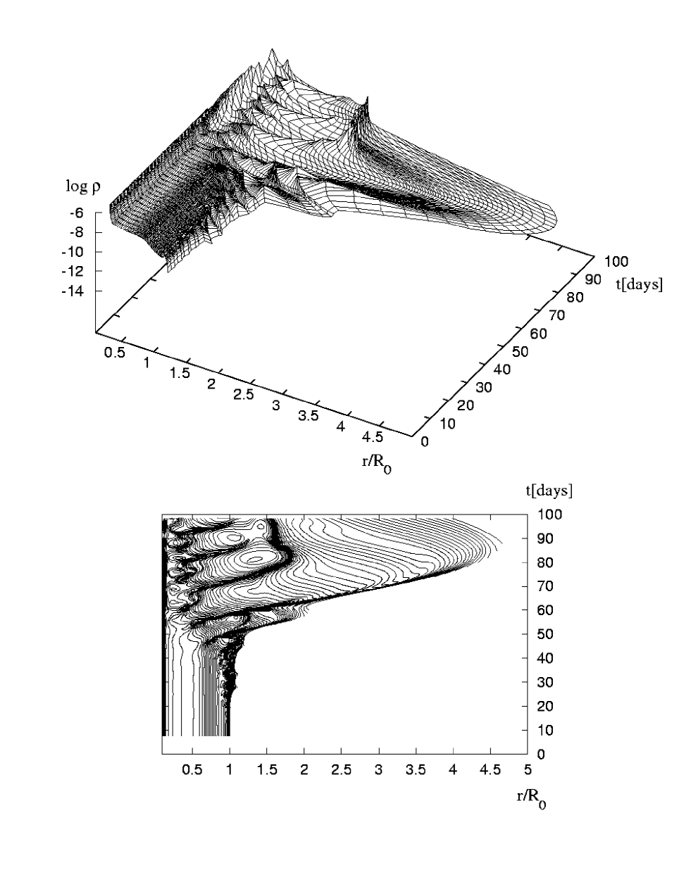
Figure 6: Density $\rho$ as a function of radius (in units of the initial radius) and time for an envelope model of P Cygni (top panel). The corresponding contour plot is given in the bottom panel. Strange mode instabilities, but no shock oscillations are resolved in these diagrams.

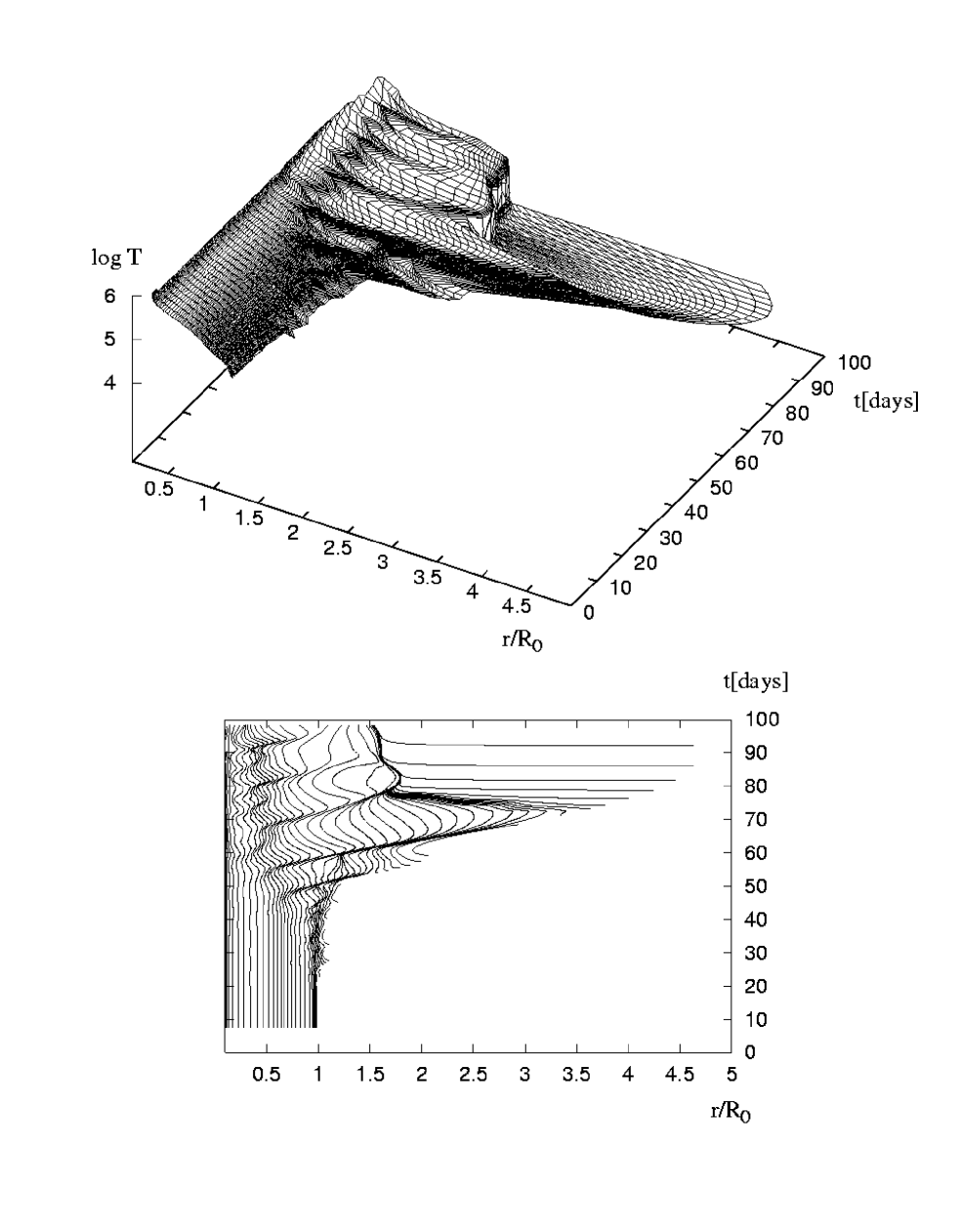
Figure 7: Same as Figure 6, but for the temperature $T$.

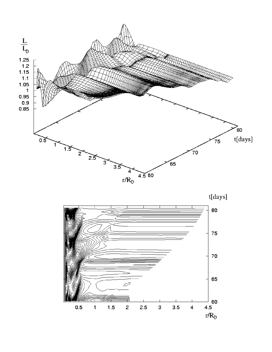
Figure 8: Luminosity in units of the initial luminosity as a function of radius (in units of the initial radius) before the shock capturing. The corresponding contour plot is given in the bottom panel. Note that the luminosity variations take place on the dynamical timescale.

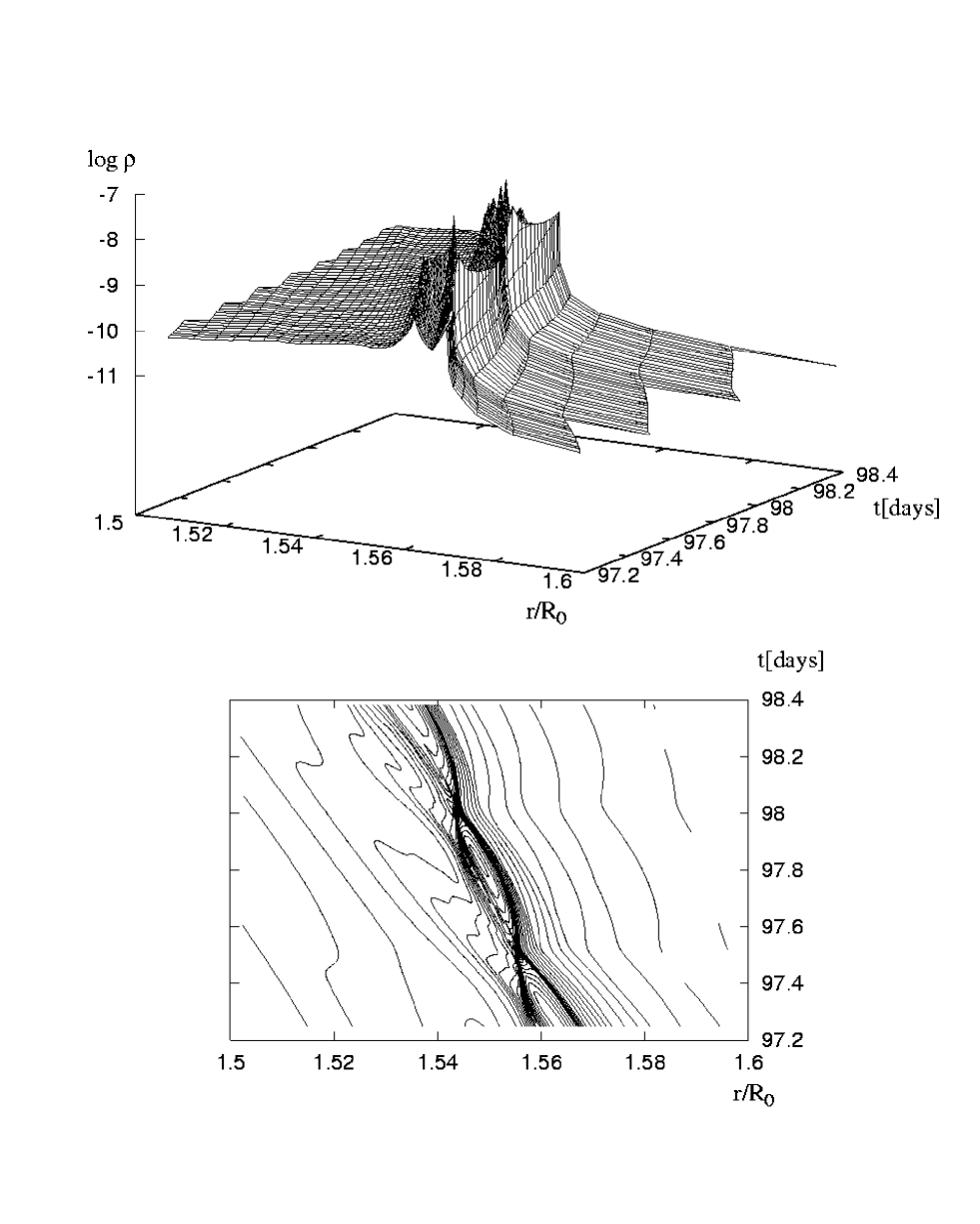
Figure 9: Same as Figure 6 in the vicinity of the captured shock and for a time interval appropriate to resolve the shock oscillations.

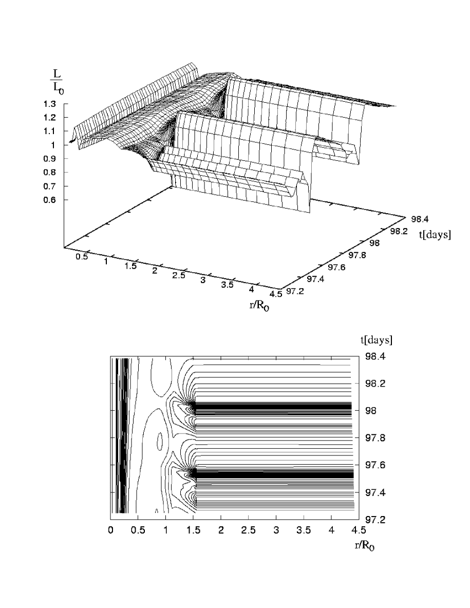
Figure 10: Luminosity in units of the initial luminosity as a function of radius (in units of the initial radius) and a time interval appropriate to resolve the shock oscillations (top panel). The corresponding contour plot is given in the bottom panel. Note that the rapid photospheric luminosity perturbations are defined at the captured shock (at $r/R_{0}\sim 1.5$). Below the shock, luminosity perturbations are governed by strange mode instabilities operating on the dynamical timescale.

We apply the method discussed above to a stellar envelope model with parameters close to those observed for the star P Cygni. Concerning luminosity, effective temperature and chemical composition for this object, various authors (Najarro, Hillier & Stahl (1997) and Pauldrach & Puls (1990)) agree that these parameters should lie in the vicinity of $L=752.5\cdot 10^{3}L_{\odot}$, $T_{\rm{eff}}=19300K$ and $X=0.31$, $Y=0.67$, $Z=0.02$. The most uncertain parameter of P Cygni is its mass. Standard stellar evolution calculations indicate a mass of $M=50M_{\odot}$ (El Eid & Hartmann (1993)), whereas spectroscopic observations are consistent with masses down to $M=23M_{\odot}$ (Pauldrach & Puls (1990)). For our simulations we adopt $M=26.5M_{\odot}$, a value supported by the observation. Even with a more conservative mass of $M=50M_{\odot}$, the model is known to be unstable with respect to strange modes (Kiriakidis, Fricke & Glatzel (1993)). The higher value of $L/M$ adopted here amplifies the tendency towards instability through shorter thermal timescales.

The simulation of strange mode instabilities in P Cygni starts from the envelope model in hydrostatic equilibrium without any external perturbations. Strange mode instabilities develop from numerical noise, pass the linear regime of exponential growth and form multiple shocks in the non-linear domain. One of these shocks is captured in the H-ionisation zone and starts oscillating on timescales of the order of the sound travel time across the front ($\sim$ 0.5 days), whereas its mean position varies on the dynamical timescale ($\sim$ 10 days). In this phase of the evolution on two different timescales domain decomposition is used to speed up the calculation considerably.

Figure 6 shows the density $\rho$ as a function of radius (in units of the initial radius) and time for the envelope model of P Cygni. The corresponding contour plot is given in the bottom panel. Note, that contour lines here and in the following are not always closed, since during the evolution of the star e.g. the density drops to values lower than those of the initial model. After reaching the non-linear regime at $t=\sim 20$ days, shocks are formed in the outer envelope, travelling outwards and inflating the envelope successively up to 4.5 initial radii. During this period, the surface velocity reaches 55 per cent of the escape velocity at $t=75$ days. After $\sim 80$ days the envelope starts to collaps, and a shock originating at $r/R\approx 0.6$ at time $t=70$ days is then captured in the H-ionisation zone around $r/R\approx 1.5$ at $t\approx 85$ days. Subsequent shocks, generated by the primary strange mode instability, are confined to the region below the captured shock.

Figure 7 is the analogue to Figure 6 for the temperature $T$. The shocks discussed above can easily be identified in the contour plot. Note the steep temperature gradient at the captured shock after its formation.

Figure 8 shows the luminosity in units of the initial luminosity as a function of radius (in units of the initial radius) and a time interval before the shock capturing. The luminosity varies on the dynamical timescale by 10 per cent, corresponding to a bolometric variation of $\sim 0.1^{\rm{m}}$. It is defined in the inner envelope and remains constant with respect to radius above. There, luminosity perturbations cannot be sustained due to the low specific heat and the associated short thermal timescales. These luminosity variations remind of the microvariations in P Cygni, described by, e.g., de Groot, Sterken & van Genderen (2001). These authors report on cyclic behaviour of the visual brightness with amplitudes of $\sim 0.1^{\rm{m}}$ and cycle lengths between 10 and 25 days, best fitting a quasi-period of $17.3^{\rm{d}}$.

Figure 9 shows the density $\rho$ as a function of radius (in units of the initial radius) in the vicinity of the captured shock and a time appropriate to resolve the shock oscillations. In particular, the corresponding contour plot in the bottom panel shows variation on two different timescales. It exhibits both shock oscillations with a mean period of $\sim$0.5 days and the evolution on the dynamical timescale, as indicated by the variation of the shock position between $r/R_{0}\approx 1.56$ and $r/R_{0}\approx 1.54$.

Figure 10 shows the luminosity in units of the initial luminosity as a function of radius (in units of the initial radius) and a time interval apropriate to resolve the shock oscillations. The rapid photospheric luminosity perturbations are defined at the captured shock (at $r/R_{0}\sim 1.5$) and remain constant above it (see discussion of Figure 8). The variation amounts to 20 per cent, corresponding to $\sim 0.2^{\rm{m}}$ bolometrically. Below the shock, luminosity perturbations are governed by strange mode instabilities operating on the dynamical timescale. The photometric luminosity perturbation is therefore a superposition of two effects, dominated by the fast oscillations induced by the shock. We emphasise, however, that the one dimensional calculations presented here have to be interpreted with caution, since massive stars are known to suffer also from non-radial instabilities (Glatzel & Mehren (1996)). Whether the captured shocks survive the deformations induced by non-radial instabilities or become unstable themselves with respect to non-radial perturbations, remains to be tested by at least two dimensional calculations. They might break apart and could then contribute to the entire variation by stochastically adding high-frequency perturbations to the cyclic perturbations on the dynamical timescale induced by strange mode instabilities. On the other hand, from the observations discussed by de Groot, Sterken & van Genderen (2001), no indications for the stability properties of the captured shock found here can be inferred, since the time resolution of the data is not sufficiently high ($\sim$ one measurement per day).

Another effect of the primary strange mode instability consists of a mass transfer from the instability region into the outer parts of the stellar envelope. Owing to the Lagrangian approach chosen here, this implies a reduced spatial resolution in the inner part of the stellar envelope. Simultaneously, grid points are concentrated around the captured shock. For reliable calculations, however, a high resolution of the instability region is indispensable. Otherwise, the physical strange mode instability generating acoustic energy and shock waves is suppressed. Thus, due to insufficient resolution, the simulation discussed had to be stopped after $\sim$100 days of simulated time. To overcome the difficulty grid reconstruction is necessary. A corresponding algorithm, consistently inserting and eliminating gridpoints during the calculation is currently being developed and will be commented on in a forthcoming publication.

5 CONCLUSIONS

Motivated by the discovery of high frequency shock oscillations in pulsating stars confined in a narrow region, we have developed a procedure for an efficient treatment of such phenomena. The integration domain is decomposed into several subdomains according to the various, vastly different timescales present in the configuration. To save computing time, these domains are integrated according to their respective timescales.

Criteria for the choice and decomposition of the computational domains have been derived. Decomposition implies artificial inner boundaries which require suitable boundary conditions. How these have to be chosen in order to minimise the numerical error (compared to the approach without decomposition) has been discussed. An overlap of the domains was found to be necessary to produce satisfactory results.

The decomposition technique has been tested and validated by comparison with results obtained without decomposition. The major effect of decomposition was found to consist of a delay in time (phaseshift) with respect to the original calculation. The latter is regarded as physically largely irrelevant. Otherwise the numerical quality of the results was proven to be satisfactory.

For the models considered, decomposition was found both theoretically and by numerical tests to reduce the computational costs by approximately a factor of two. The speed-up critically depends on the size of the rapidly varying domain. Although a reduction of computing time by 50 per cent sounds moderate, it is of practical relevance considering the duration of several weeks for a complete simulation. The intended extension of the procedure to two dimensional problems will yield an appreciably higher speed-up than that for the one dimensional model considered here, since the iterative inversion of some matrices there requires of the order of $N^{2}$ operations. Moreover, decomposition in two dimensions may reduce the size of matrices to be inverted such that fast direct methods (requiring of the order of $N$ operations) become most efficient, whose application would then imply a further acceleration of the computation.

We have applied the method to a model for the star P Cygni, paying special attention to the adequate treatment of the different timescales involved.

References

- Ardelyan & Gushchin (1982) Ardelyan N., Gushchin I., 1982, Moscow Univ. Comp. Math. and Cybernetics, 3, 3
- Baker & Kippenhahn (1965) Baker N.H., Kippenhahn R., 1965, ApJ, 142, 869
- Cox (1980) Cox J.P., 1980, Theory of Stellar Pulsation. Princeton Univ. Press, Princeton, NJ
- Dorfi & Gautschy (2000) Dorfi E. A., Gautschy A., 2000, ApJ, 545, 982
- El Eid & Hartmann (1993) El Eid M.F., Hartmann D., 1993, ApJ, 404, 271
- Fraley (1968) Fraley, G.S., 1968, Ap&SS, 2, 96
- Glatzel & Kiriakidis (1993) Glatzel W., Kiriakidis M. 1993, MNRAS, 263, 375
- Glatzel, Kiriakidis, Chernigovskij & Fricke (1999) Glatzel W., Kiriakidis M., Chernigovskij S., Fricke K.J. 1999, MNRAS, 303, 116
- Glatzel & Mehren (1996) Glatzel W., Mehren S. 1996, MNRAS, 282, 1470
- de Groot, Sterken & van Genderen (2001) de Groot M., Sterken C., van Genderen A.M., 2001, A&A, 376,224
- Grott, Glatzel & Chernigovski (2002) Grott M., Glatzel W., Chernigovski S., 2002, MNRAS, submitted
- Humphreys R.M. & Davidson K. (1979) Humphreys R.M., Davidson K., 1979, ApJ, 232, 409
- Humphreys R.M. & Davidson K. (1994) Humphreys R.M., Davidson K., 1994, PASP, 106, 704
- Iglesias, Rogers & Wilson (1992) Iglesias C.A., Rogers F.J., Wilson B.G., 1992, ApJ, 397, 717
- Kiriakidis, Fricke & Glatzel (1993) Kiriakidis M., Fricke K.J., Glatzel W. 1993, MNRAS, 264, 50
- Najarro, Hillier & Stahl (1997) Najarro F., Hillier D.J., Stahl O., 1997, A&A, 326, 1117
- Pauldrach & Puls (1990) Pauldrach A.W.A., Puls J., 1990, A&A, 237, 409
- Rogers & Iglesias (1992) Rogers F.J., Iglesias C.A., 1992, ApJS, 79, 507
- Samarskii & Popov (1969) Samarskii A., Popov Yu., 1969, Zh. Vychisl. Mat. i Mat. Fiz., 9, 953
- Samarskii et. al. (1981) Samarskii A., Tishkin V., Favorskii A., Shashkov M., 1981, Diff. Eqns., 17, 854
- Shashkov (1996) Shashkov M., 1996, Conservative Finite-Difference Methods on General Grids, CRC Press, New York
- Wu (1999) Wu Z., 1999, SIAM J. Sci. Comput., 20, 5, 1851
- Wu & Zou (2000) Wu Z., Zou H., 2000, J. Comp. Phys., 157, 2