Analytic solutions for spherical gravitational gas accretion on to a solid body

Abstract

The process of gravitational accretion of initially homogeneous gas onto a solid ball is studied with methods of fluid dynamics. The fluid partial differential equations for polytropic flow can be solved exactly in an early stage, but this solution soon becomes discontinuous and gives rise to a shock wave. Afterwards, there is a crossover between two intermediate asymptotic self-similar regimes, where the shock wave propagates outwards according to two similarity laws, initially accelerating, then decelerating (and eventually vanishing). Lastly, we study the final static state. Our purpose is to attain a global picture of the process.

1 Introduction

The problem of spherical infall of gas onto a solid object has application in several astrophysical situations. For example, it can represent the infall of gas onto a neutron star from the surrounding cloud. Alternatively, it can be a simplified model for the formation of planetary atmospheres as a result of gas accretion onto the solid (rock) surface of a previously formed spherical core.

Aspects of this fluid dynamical problem have been treated before in the literature. A simplified formulation with constant gravity was considered by Bisnovatyi-Kogan, Zel’dovich & Nadezhin (1972) and a self-similar solution with a shock wave found. Self-similar solutions with the (variable) gravity due to a central point-like mass, applicable to either ordinary or neutron stars, were studied by Cheng (1977). Similarity methods favour power-law distributions. This property was amply used in the study of supernova explosion and later fallback by Chevalier (1989). An extensive study of self-similar spherical accretion with an initial power-law radial distribution of gas was provided by Kazhdan & Murzina (1994). They concluded that a realistic solution should be an interpolation between a self-similar solution with zero mass flux near the origin (of which they derived general features) and a solution with constant gravity and the correct boundary conditions at the solid surface.

Chevalier (1989) and Kazhdan & Murzina (1994) assume that the incident gas flow is cold ($T=0$) and, respectively, that its accretion rate decays with time with some exponent or that its density decays with radius with exponent $\omega<3$ (both conditions are related). A cold inflow is not a good approximation for large distances where the gas thermal energy is non-negligible with respect to its gravitational energy. On the other hand, the condition $\omega<3$ implies that the mass of gas diverges at large radius, making the neglect of its self gravity questionable.

One may try to amend these problems by endowing the incident gas with pressure. For polytropic flow, similarity demands that the initial pressure be also a power law with radius and, furthermore, determines the exponents (in terms of the polytropic exponent). This is the case studied by Cheng (1977) and it may seem somewhat unnatural. Besides, the exponent of the density distribution also leads to diverging mass with radius and, hence, to the self-gravity problem.

In this paper, we relax the demand of having similarity at the ouset and consider instead simple uniform initial conditions for the gas. In other words, the initial configuration is a solid body with a spherically symmetric mass distribution (a ball) placed in a homogeneous gas with pressure, and the problem is to analyze the subsequent evolution of this gas under the body’s gravity. The evolution will consist of infall of gas with a progressive modification of the gas distribution around the body, while the gas stays homogeneous far from it. This is essentially the type of accretion treated by Bondi (1952), although the artificial imposition of stationary flow allowed him to dispense with differential equations. At any rate, a homogeneous distribution of gas is just a particular case of power law ($\omega=0$) and, therefore, comparison with the results of Chevalier (1989) and Kazhdan & Murzina (1994) will be possible.

These simple initial conditions are suitable for an analytic treatment, employing the full power of the methods of nonlinear fluid dynamics. These allow us to attain a clear picture of the initial non-trivial process near the surface. In particular, the exact description of the formation of a shock wave may illustrate its general features in accretion processes. Even though the evolution is not self similar, similarity arises in the course of it, and we shall see how and why. Due attention is also paid to the self-gravity question, and to the decay towards a final static state.

This paper is organized as follows. In section 2, we introduce the relevant magnitudes in the problem and, hence, various space and time scales, to reach a rough intuitive idea of the physics involved and to define the limits of applicability of the model. In section 3, we introduce the fluid equations to be used. In section 4, an exact solution is found for the initial non-trivial dynamics, which occurs near the ball’s surface. In the following section we obtain two similarity solutions valid for larger $t$, the first still confined within a short distance from the ball, while the second is valid for large radius. Finally we consider the long-time asymptotic static state and discuss the results.

A note on notation: we shall use frequently the asymptotic signs $\sim$ and $\approx$; for example, $f(x)\sim g(x)$ or $f(x)\approx g(x)$ (sometimes without making explicit the independent variable $x$). The former means that $\lim f(x)/g(x)$ when $x$ goes to zero or infinity, as the case may be, is finite, while the latter means, in addition, that the limit is one. On the other hand, the sign $\sim$ may appear in some instances with the related but looser meaning “equal up to a numerical factor of the order of unity”.

2 Relevant magnitudes and dimensional analysis

The initial condition (the solid ball in the homogeneous gas) is characterized by four parameters, namely, the radius $R$ and mass $M$ of the ball, and the pressure $P_{0}$ and density $\rho_{0}$ of the gas (we assume that the gas is perfect, inviscid, and non-heat-conducting or polytropic). In addition, we have the constant of gravity $G$. From these five dimensional characteristic parameters, we can form two independent non-dimensional numbers, namely, the ratio of densities $(4/3)\pi R^{3}(\rho_{0}/M)$ and the ratio $RP_{0}/(\rho_{0}GM)$. The quantity $P_{0}/\rho_{0}\sim c_{0}^{2}$ ($c_{0}$ being the sound speed) is approximately the gas thermal energy per unit of mass. On the other hand, $GM/R$ is the gas potential energy per unit of mass on the ball. Their ratio measures the relative strength of gravity in our problem. To have any significant gas infall, we must demand that the ball’s gravity dominates over the gas thermal energy, that is, $Rc_{0}^{2}/(GM)\ll 1$. The ratio of densities is also very small. This is a necessary condition for neglecting the self-gravity of the gas, as we will do, but it is not sufficient. We shall discuss the sufficient condition after analysing the typical length and time scales.

The basic length scale is $R$, of course. We can get a larger length scale by dividing by the small number $Rc_{0}^{2}/(GM)$:

$${\cal R}:={R\over Rc_{0}^{2}/(GM)}={GM\over c_{0}^{2}}.$$ (1)

This length ${\cal R}$ marks the scale at which the gas thermal energy is similar to its potential energy. It was introduced by Bondi (1952) to define a non-dimensional radial variable. Alternatively, we may divide $R$ by the cubic root of the other small number $(4/3)\pi R^{3}(\rho_{0}/M)$:

$${R\over R[(4/3)\pi(\rho_{0}/M)]^{1/3}}=\left({3\over 4\pi}{M\over\rho_{0}}\right)^{1/3},$$ (2)

in which we may suppress the numerical factor. Obviously, this second length is the radius of a volume of gas such that its mass is similar to $M$.

Analogously, we have a basic time scale, namely, $R^{3/2}/\sqrt{GM}$, defined only in terms of the ball’s parameters (and interpreted as the typical time of Keplerian motion close to the ball’s surface). Dividing by $[Rc_{0}^{2}/(GM)]^{3/2}$ we cancel the $R$ dependence and obtain $GM/c_{0}^{3}$, that is, the time of sound propagation over the distance ${\cal R}$ (note that the time of Keplerian motion at distance ${\cal R}$ is ${\cal R}^{3/2}/\sqrt{GM}=GM/c_{0}^{3}$ as well). Finally, dividing by $[R^{3}(\rho_{0}/M)]^{1/2}$, we cancel both the $R$ and $M$ dependences and obtain $1/\sqrt{G\rho_{0}}$, the typical time of gravitational collapse of the gas (aside from the ball, which might act as a seed for the collapse).

We will assume that the largest typical length (the radius of a mass of gas $M$) is much larger than the intermediate scale ${\cal R}$; in other words, we consider the mass of gas in the volume of radius ${\cal R}$ negligible in comparison with $M$. Then, analogously, the typical time of gas collapse is much larger than $GM/c_{0}^{3}$. This is the precise condition for neglecting the self-gravity of the gas, understood in an asymptotic sense, namely, ${\cal R}\ll(M/\rho_{0})^{1/3}$ or $GM/c_{0}^{3}\ll 1/\sqrt{G\rho_{0}}$. In non-dimensional form, $c_{0}^{6}/(G^{3}M^{2}\rho_{0})\gg 1$, which can be restated in terms of the two previously defined non-dimensional numbers: besides that both must be very small, the ratio

$${R^{3}\rho_{0}\over M}:\left({Rc_{0}^{2}\over GM}\right)^{3}=\left({{\cal R}\over R}\right)^{3}{R^{3}\rho_{0}\over M}\ll 1,$$ (3)

that is, the ratio of densities must be much smaller than the other one. Interestingly, under this condition, the parameters $M$ and $G$ will not appear independently in the equations of motion but only in the combination $GM$, so that one has only four dimensional parameters. Correspondingly, only one non-dimensional number is relevant, namely, the ratio $R/{\cal R}$.

As regards mass scales, the basic mass is $M$, of course. The mass of gas enclosed in the sphere of radius ${\cal R}$, namely, ${\cal M}\approx(4/3)\pi{\cal R}^{3}\rho_{0}$, can be interpreted as the total mass of initially bound gas. We observe that ${\cal M}/M\sim{\cal R}^{3}\rho_{0}/M\ll 1$, according to condition (3). On the other hand, this condition can also be written as $M_{J}\gg M$, introducing the gas Jeans mass $M_{J}\sim c_{0}^{3}/(G^{3}\rho_{0})^{1/2}$. This is, of course, the natural mass scale for gas collapse due to self gravity.

It is convenient to remark that, since we still have after neglecting the gas self gravity one non-dimensional number $(R/{\cal R})$, we can construct many length and time scales (large or small), but they have no particular physical meaning. However, multiplying the basic length $R$ by that number, we obtain $R^{2}c_{0}^{2}/(GM)=c_{0}^{2}/g$, where $g$ is the gravity on the ball’s surface. This small length scale and its associated time scale $c_{0}/g$ will play a rôle in the sequel.

3 Fluid equations

Under the assumption of spherical symmetry, we are led to solving the partial differential equations of fluid dynamics in one dimension (the radial distance). These equations are nonlinear and no general method of solution is available. However, given the simplicity of the initial and boundary conditions, many results can be obtained by purely analytic means, as we shall see.

We consider an adiabatic evolution of the gas or, more generally, a polytropic equation of state, $P\propto\rho^{\gamma}$ ($\gamma\geq 1$). Then, we have the continuity equation, the Euler equation and the thermodynamic equation:

$${\partial\rho\over\partial t}+{\partial(\rho v)\over\partial x}+{2(\rho v)\over x}=0,$$ (4)

$${\partial v\over\partial t}+v{\partial v\over\partial x}=-g-{1\over\rho}{\partial P\over\partial x},$$ (5)

$${\partial\over\partial t}{P\over\rho^{\gamma}}+v{\partial\over\partial x}{P\over\rho^{\gamma}}=0,$$ (6)

where $g=GM/x^{2}$ is the gravity acceleration (Chevalier 1989; Kazhdan & Murzina 1994). The initial conditions are: $\rho(0,x)=\rho_{0}$, $P(0,x)=P_{0}$ and $v(0,x)=0$ ($x\geq R$). The boundary condition at the solid surface is $v(t,R)=0$.

In principle, Eq. (6) has the trivial solution $P/\rho^{\gamma}=P_{0}/\rho_{0}^{\gamma}$. Let us introduce the sound velocity $c$, which satisfies

$$c^{2}(\rho)/c_{0}^{2}=(\rho/\rho_{0})^{\gamma-1}\quad(c_{0}^{2}=\gamma P_{0}/\rho_{0}).$$ (7)

Hence, the mathematical problem boils down to solving

$${\partial\rho\over\partial t}+{\partial(\rho v)\over\partial x}+{2(\rho v)\over x}=0,$$ (8)

$${\partial v\over\partial t}+v{\partial v\over\partial x}=-g-{c^{2}(\rho)\over\rho}{\partial\rho\over\partial x}.$$ (9)

The polytropic gas flow in one dimension is amenable to powerful mathematical methods (Courant & Friedrichs, 1948; Landau & Lifshitz 1987; Chorin & Marsden 1993), although the presence of gravitation complicates the problem. However, restricting our interest to a small zone near the surface, we can take the acceleration of gravity $g$ constant in Eq. (9) (Bisnovatyi-Kogan, Zel’dovich & Nadezhin 1972). This will allow us to take advantage of those methods.

4 Initial stages

Initially, the gas will start falling with acceleration $g$, that is, with a negative velocity increasing as $v\approx-g\,t$. However, it will be stopped at the ball’s surface, where the density and, therefore, the pressure must increase. Consequently, a wave transmitting the boundary condition $v(t,R)=0$ will propagate outwards. It is therefore crucial to determine the law of propagation of waves in the present conditions. This is called, in mathematical terms, the analysis of characteristics. Once this is done, and as long as the dynamics consists of the propagation of a simple wave, one can obtain an exact solution. It is not possible here to describe in detail how this solution is obtained and our focus will be the origin of the shock wave. We refer the reader to Courant & Friedrichs (1948), Landau & Lifshitz (1987) or Chorin & Marsden (1993) for a general treatment of the theory of one-dimensional gas flow.

For the moment, we confine ourselves to a spherical shell over the surface of height much smaller than $R$, where we can consider $g$ constant. Hence, the problem becomes that of the fall of gas on a flat surface (the ground) and it is convenient to take this surface as the origin of $x$. So we must use the one-dimensional form of the vector divergence and, therefore, we must neglect the last term on the left-hand side of the continuity equation (8), writing it as

$${\partial\rho\over\partial t}+{\partial(\rho v)\over\partial x}=0.$$ (10)

The gas still unperturbed by the wave merely falls with velocity $v=-g\,t$. In a reference system falling with it, it is at rest and, therefore, the speed of sound is $c_{0}$. Hence, in the original reference system the wave front is located at $x_{f}=c_{0}t-g\,t^{2}/2$. Then, for $x>x_{f}$, the solution is trivial, and we only need to find the solution for $x<x_{f}$. In the falling frame, the acceleration of gravity vanishes and the set of two equations (10) and (9) reduces to a “gas tube problem” that can be solved by introduction of the Riemann invariants (Courant & Friedrichs, 1948; Landau & Lifshitz 1987; Chorin & Marsden 1993). Let us denote $x^{\prime},v^{\prime},c^{\prime}$ the coordinate and variables in this frame. Initially, we have a constant state, which is preserved for $x^{\prime}\geq x^{\prime}_{f}=c_{0}t$. The backward characteristics crossing the forward characteristic $x^{\prime}=c_{0}t$ transmit a constant value of the Riemann invariant $J_{-}$, so the solution is a forward simple wave. Given that

$$J_{-}=v^{\prime}-\frac{2c^{\prime}}{\gamma-1}=-\frac{2c_{0}}{\gamma-1},$$

the sound velocity is related with the gas velocity by $c^{\prime}=c_{0}+(\gamma-1)v^{\prime}/2$. Furthermore, the fact that the solution is a forward simple wave implies that the forward characteristics are straight lines. Hence, the wave’s propagation law $v^{\prime}=F(x-c^{\prime}\,t)$ is an implicit equation for $v^{\prime}$, assuming that we can determine the function $F$. This is done using the boundary condition $v(t,0)=0$. The implicit equation is algebraic and its solution is straightforward. We then obtain:

$$v(x,t)=\left\{{\begin{array}[]{l}-gt,\quad x\geq c_{0}t-{g\over 2}t^{2}\\ -{c_{0}\over\gamma}-{\gamma-1\over 2\gamma}gt+\sqrt{\left({c_{0}\over\gamma}+{\gamma-1\over 2\gamma}gt\right)^{2}-{2g\over\gamma}x},\\ \hbox{\hskip 113.81102pt}x\leq c_{0}t-{g\over 2}t^{2}.\end{array}}\right.$$ (11)

For a simple wave, the density is a definite function of the velocity. We can calculate it from Eq. (7) to be

$$\rho(x,t)=\rho_{0}\left[1+{\gamma-1\over 2}\,{v(x,t)+gt\over c_{0}}\right]^{{2\over\gamma-1}}.$$ (12)

These expressions for $\rho$ and $v$ constitute the solution of Eqs. (9) and (10) with the given boundary conditions.

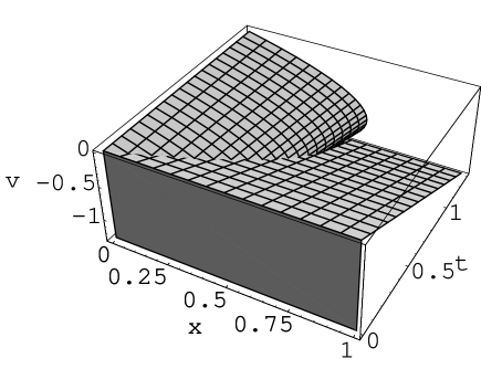
Figure 1: Evolution of the velocity in the early stages in non-dimensional units ($c_{0}=g=1$) for $\gamma=7/5$, displaying how it becomes multivalued, hence giving rise to a shock wave.

The alert reader may have noted a peculiarity of the solution found above: the wave front’s coordinate $x_{f}$ begins increasing but, for $t>c_{0}/g$, changes to decreasing and, eventually, returns to the origin (free fall with initial velocity $c_{0}$). On the other hand, a simple analysis shows that a singularity occurs before, namely, a shock wave. One can calculate $(\partial x/\partial v)_{t}$, and its null locus defines a line in the $xt$-plane, namely, $x=[2c_{0}+(\gamma-1)gt]^{2}/(8\gamma g)$. Initially, the corresponding $x$ is larger than $x_{f}$, so it is unphysical, but, for $t=2c_{0}/[(\gamma+1)g]$, it meets the wave front; that is, the falling gas overtakes the gas just below it and a shock wave develops henceforth. From that moment onwards, the solution (11,12) becomes multivalued and ceases to be valid (see Fig. 1). Although it is possible, in principle, to study the situation in which a shock wave propagates, the analysis cannot be done in terms of a simple wave and it is far more complicated.

Of course, the foregoing analysis is valid as long as everything happens in a thin shell, which implies that the typical length $c_{0}^{2}/g\ll R$, equivalent to ${\cal R}\gg R$ (the already mentioned condition of gravity dominated evolution).

5 Similarity solutions

A one-dimensional gas flow problem may be formulated with similarity variables [in which the fluid partial differential equations become ordinary differential equations (ODEs)] only when the initial and boundary conditions are sufficiently simple (Sedov 1982). Certainly, this is not our case, for we can construct independent length and time scales (see section 2). Nevertheless, it is commonly observed that nonlinear equations that do not have similarity solutions at the outset develop them in an intermediate asymptotic regime, that is, a regime between two very different scales where both scales can be neglected (Barenblatt 1996). We will actually find two independent intermediate asymptotic regimes.

We shall study first the self similar solution that develops from the exact solution found in section 4, that is, with constant gravity. The corresponding ODE have been formulated by Bisnovatyi-Kogan, Zel’dovich & Nadezhin (1972). However, we shall derive a slightly different (though equivalent) system of equations more amenable to analytic study.

Afterwards, we proceed to consider the variation of gravity with radius, connecting with the similarity solutions of Chevalier (1989) and Kazhdan & Murzina (1994). These solutions are for an initial density distribution given by $\rho=B\,x^{-\omega}$ but a constant density is just a particular case. The most interesting solutions is the one with zero mass flux near the origin, named “of type 3” (Kazhdan & Murzina 1994), since it is expected to match the self-similar solution with constant gravity.

5.1 Constant gravity

In this case, we have one less parameter, because the parameters $R$ and $GM$ only appear in the combination $g=GM/R^{2}$. However, we can still form the two independent non-dimensional variables $gt/c_{0}$ and $gx/c_{0}^{2}$, so we will have to remove another parameter to have a similarity solution. If we assume that the initial gas temperature is very low, then $c_{0}\rightarrow 0$ and the only possible non-dimensional variable is $\xi=x/(gt^{2})$ (or a function of it). (We measure the distance $x$ from the ground.) This corresponds to the intermediate asymptotics $c_{0}^{2}/g\ll x\ll R$; equivalently, in terms of the non-dimensional height variable $\tilde{x}=gx/c_{0}^{2}$, it corresponds to $1\ll\tilde{x}\ll{\cal R}/R$ (recall that ${\cal R}\gg R$).

To take into account the presence of shock waves and the consequent dissipation, we consider the full set of equations (5), (6) and (10). We can express them in non-dimensional form by introducing new variables:

$$v={x\over t}u,\quad\rho=\rho_{0}r,\quad P={x^{2}\over t^{2}}\,\rho_{0}\,p.$$ (13)

Some straightforward algebra then yields,

$$\xi[u^{\prime}+(u-2){r^{\prime}\over r}]+u=0,$$ (14)

$$(u-2)\,\xi u^{\prime}+u^{2}-u=-\xi^{-1}-r^{-1}(2p+\xi p^{\prime}),$$ (15)

$$(u-2)\,\xi[\ln(p/r^{\gamma})]^{\prime}+2(u-1)=0.$$ (16)

Upon making the change of variables

$$\left\{{\begin{array}[]{l}\xi=\tilde{\xi}-{1\over 2},\\ u={\tilde{\xi}\tilde{u}-1\over\xi},\\ p={\tilde{\xi}^{2}\tilde{p}\over\xi^{2}}\end{array}}\right.$$ (17)

(corresponding to changing to the falling reference frame), the $\xi^{-1}$ term in the second equation vanishes and the system of ordinary differential equations simplifies to

$$\tilde{\xi}[\tilde{u}^{\prime}+(\tilde{u}-2){r^{\prime}\over r}]+\tilde{u}=0,$$ (18)

$$(\tilde{u}-2)\,\tilde{\xi}\tilde{u}^{\prime}+\tilde{u}^{2}-\tilde{u}=-r^{-1}(2\tilde{p}+\tilde{\xi}\tilde{p}^{\prime}),$$ (19)

$$(\tilde{u}-2)\,\tilde{\xi}[\ln(\tilde{p}/r^{\gamma})]^{\prime}+2(\tilde{u}-1)=0.$$ (20)

Bisnovatyi-Kogan, Zel’dovich & Nadezhin (1972) do not make the change to the falling reference frame, and restrict themselves to solving the equations by a series expansion near the ground. Instead, after the change of reference, we can follow the general (and more powerful) methods exposed by Sedov (1982). In particular, we note that in terms of the variable $\tau=\ln\tilde{\xi}$, the previous equations constitute a system of autonomous nonlinear ODE, namely,

$${d\tilde{u}\over d\tau}={\frac{\tilde{p}(\tau)\,\left[2+\gamma\,\tilde{u}(\tau)\right]-r(\tau)\,\tilde{u}(\tau)\left(2-3\,\tilde{u}(\tau)+{{\tilde{u}(\tau)}^{2}}\right)}{-\gamma\,\tilde{p}(\tau)+r(\tau)\,{{\left[\tilde{u}(\tau)-2\right]}^{2}}}},$$ (21)

$${dr\over d\tau}=r(\tau){\frac{-2\,\tilde{p}(\tau)+r(\tau)\,\left[\tilde{u}(\tau)-2\right]\,\tilde{u}(\tau)}{\left(-\gamma\,\tilde{p}(\tau)+r(\tau)\,{{\left[\tilde{u}(\tau)-2\right]}^{2}}\right)\,\left[\tilde{u}(\tau)-2\right]}},$$ (22)

$${d\tilde{p}\over d\tau}=\tilde{p}(\tau){\frac{2\,\gamma\,\tilde{p}(\tau)-r(\tau)\,\left(4-\left(6+\gamma\right)\,\tilde{u}(\tau)+2\,{{\tilde{u}(\tau)}^{2}}\right)}{-\gamma\,\tilde{p}(\tau)+r(\tau)\,{{\left[\tilde{u}(\tau)-2\right]}^{2}}}}.$$ (23)

One can study this system of equations with the methods of nonlinear ODE, that is, study its singular points, phase portrait, etc. However, given the homogeneity properties of these equations with respect to $\tilde{p}$ and $r$, it proves convenient to introduce the variable $\tilde{\theta}=\tilde{p}/r$. It is (in the falling frame) the non-dimensional form of the temperature for the perfect gas with pressure $P$ and density $\rho$, that is, $T=\mu\,(x^{2}/t^{2})\,\theta$ ($\mu$ being the molar mass and $T$ being measured in energy units). Hence,

$${d\tilde{\theta}\over d\tilde{u}}=\tilde{\theta}\,{\frac{2\,\tilde{\theta}\,\left(1+\gamma\,(\tilde{u}-2)\right)-\left(\tilde{u}-2\right)\,\left(4-\left(5+\gamma\right)\,\tilde{u}+2\,{{\tilde{u}}^{2}}\right)}{\left(\tilde{u}-2\right)\,\left(\tilde{\theta}\,\left(2+\gamma\,\tilde{u}\right)-\tilde{u}\,\left(2-3\,\tilde{u}+{{\tilde{u}}^{2}}\right)\right)}}$$ (24)

The solution of this equation provides the relation between the “velocity” $\tilde{u}$ and the “temperature” $\tilde{\theta}$, $\tilde{\theta}({\tilde{u}})$. Substituting it back into Eq. (21), we have an ODE for ${\tilde{u}}(\tau)$, which is immediately solved by a quadrature. Analogously, one solves for $r(\tau)$.

To solve the nonlinear ODE (24), let us note that we are actually interested in some particular initial conditions, derived from the initial and boundary conditions of the original partial differential equations (PDE). The initial conditions for the PDE are given at $t=0$, that is, at $\tilde{\xi}=\xi=\infty$. They are $\rho(0,x)=\rho_{0}$, $P(0,x)=P_{0}=0$ ($c_{0}\rightarrow 0$) and $v(0,x)=0$, implying that $r=1$ and $u=0$. The boundary condition for the PDE is given at $x=0\Rightarrow\xi=0$ and $\tilde{\xi}=1/2$, where $v=0$. Since $v=gt(\tilde{\xi}\tilde{u}-1)$, it implies that $\tilde{u}=2$.

Let us see if we have gathered enough information to determine a unique solution of Eq. (24). Given that $\tilde{\theta}\rightarrow 0$ as $\tilde{\xi}\rightarrow\infty$, this must be a fixed point. There are three singular points of Eq. (24) with $\tilde{\theta}=0$, namely, with $\tilde{u}=0,$ 1 or 2, respectively. If we want to have a finite $v$ as $x\rightarrow\infty$, we must take the point $(0,0)$. So we know that the solution of Eq. (24) that we seek must end at the origin. On the other hand, the singular point $(2,0)$ corresponds to the boundary conditions at $x=0$. However, the solution that departs from this point does not end at the origin (see Fig. 2). This does not mean that there is an inconsistency, for there can be discontinuities in the solution. Indeed, in most self-similar solutions the boundary conditions can only be fulfilled if there is a point of discontinuity (Sedov 1982).

Therefore, recalling the exact solution of section 4, we observe that a shock wave arises and propagates upwards. Then we must consider discontinuities associated to the presence of a shock wave. The conditions for conservation of mass, momentum and energy across a shock surface read (Courant & Friedrichs, 1948; Landau & Lifshitz 1987; Chorin & Marsden 1993)

$$\left\{{\begin{array}[]{l}\rho_{1}v_{1}=\rho_{2}v_{2},\\ P_{1}+\rho_{1}v_{1}^{2}=P_{2}+\rho_{2}v_{2}^{2},\\ {v_{1}^{2}\over 2}+w_{1}={v_{2}^{2}\over 2}+w_{2},\end{array}}\right.$$ (25)

where subindices refer to the values on each side of the shock and $w$ is the enthalpy (or the appropriate thermodynamic function for general $\gamma$); for a perfect gas, $w=\gamma P/[\rho(\gamma-1)]$. These equations hold in a coordinate system in which the shock surface is at rest. On the other hand, the location of the shock must be at fixed $\xi$, say $\xi_{s}$. Consequently, the shock wave velocity is

$$v_{s}={dx_{s}\over dt}=\xi_{s}g{dt^{2}\over dt}=2\xi_{s}gt=2{x_{s}\over t},$$

that is, $u_{s}=2$. Then,

$$\left\{{\begin{array}[]{l}r_{1}(u_{1}-2)=r_{2}(u_{2}-2),\\ p_{1}+r_{1}(u_{1}-2)^{2}=p_{2}+r_{2}(u_{2}-2)^{2},\\ {(u_{1}-2)^{2}\over 2}+{\gamma\over\gamma-1}{p_{1}\over r_{1}}={(u_{2}-2)^{2}\over 2}+{\gamma\over\gamma-1}{p_{2}\over r_{2}},\end{array}}\right.$$ (26)

valid in both the rest and the falling reference frames. Using the falling frame and eliminating $r_{2}/r_{1}$ between the first and second equations,

$$\left\{{\begin{array}[]{l}{\tilde{\theta}_{1}\over\tilde{u}_{1}-2}+\tilde{u}_{1}-2={\tilde{\theta}_{2}\over\tilde{u}_{2}-2}+\tilde{u}_{2}-2,\\ (\tilde{u}_{1}-2)^{2}+{2\gamma\over\gamma-1}\tilde{\theta}_{1}=(\tilde{u}_{2}-2)^{2}+{2\gamma\over\gamma-1}\tilde{\theta}_{2}.\end{array}}\right.$$ (27)

We have arrived at an involutive mapping of the plane $({\tilde{u}},\tilde{\theta})$ as the relation between the variables at either side of the shock discontinuity. Since we have the condition that as $x\rightarrow\infty$ the solution goes to $(0,0)$ and (in the falling frame) these values hold all the way down to the shock surface, we just need the image of the origin under the mapping. This yields the point

$$({\frac{4}{\gamma+1}},{\frac{8\,\left(\gamma-1\right)}{{{\left(\gamma+1\right)}^{2}}}}).$$

Therefore, we need the solution of Eq. (24) that goes through this point. We can see in an example (Fig. 2) that the strand of this solution that we need ends at the point (2,0), hence satisfying the boundary condition at $x=0$.

Now, substituting the function just computed back into Eq. (21), we obtain

$$d\tau={\frac{\gamma\,{\tilde{\theta}}(\tilde{u})-{{\left(\tilde{u}-2\right)}^{2}}}{-\theta(\tilde{u})\,\left(2+\gamma\,\tilde{u}\right)+\tilde{u}\,\left(2-3\,\tilde{u}+{{\tilde{u}}^{2}}\right)}}\,d\tilde{u},$$ (28)

from which we can deduce the interval of $\tau$ between the points $\left(4/(\gamma+1),8\left(\gamma-1\right)/{\left(\gamma+1\right)}^{2}\right)$ and (2,0) by integration. The result for $\gamma=7/5$ (the adiabatic index of a perfect diatomic gas) is 0.0880104. Hence, we obtain the quotient between the corresponding values of $\tilde{\xi}$. This quotient gives the location of the shock relative to the ground: recovering the original notation that distinguishes both reference frames, ${\tilde{\xi}}_{s}/(1/2)=\exp 0.0880104=1.09200\Rightarrow\xi_{s}=0.0919995/2=0.0459997$, so that the coordinate of the shock is $x_{s}=0.0459997\,gt^{2}$.

Figure 2: Relevant solution of the ODE (24) for $\gamma=7/5$, displaying the origin and its image at the shock surface, the point $(5/3,5/9)$.

It is easy to compute the post-shock $u$ in the rest frame: $u=[(1.092/2)(5/3)-1)]/0.046=-1.957$. Hence, the post-shock velocity is $v=(x_{s}/t)\,u=\xi_{s}u\,gt=-0.09gt$. Comparing with the pre-shock value $v=-gt$, we see a great reduction. The corresponding kinetic energy is dissipated as heat. The similarity properties of the velocity and its jump at the shock are shown in Fig. 3.

The ratio of post-shock to pre-shock densities can be derived from the first Eq. (26) as $\rho_{2}/\rho_{1}=(\gamma-1)/(\gamma+1)=6$, as corresponds to “strong shocks” (Landau & Lifshitz 1987). The post-shock temperature is given by $T=\mu(x_{s}^{2}/t^{2})\theta=\mu\left(8\left(\gamma-1\right)/{\left(\gamma+1\right)}^{2}\right){\tilde{\xi}}_{s}^{2}g^{2}t^{2}=0.166\,\mu g^{2}t^{2}\Rightarrow T/T_{0}=0.232\,(gt/c_{0})^{2}$. Therefore, the post-shock pressure, $P=\rho\,T/\mu$, is not polytropic.

Other properties of the self-similar solution found are worth noting, but require further analysis of the ODE system (21, 22, 23). For example, at the ground, $\tilde{\theta}=\xi^{2}\theta/{\tilde{\xi}}^{2}=0$, so that $\theta=\lim_{\xi\rightarrow 0}\tilde{\theta}/(4{\xi}^{2})$. To calculate this limit we need to know the behaviour of $\tilde{\theta}$ near $\xi=0$ ($\tau=-\ln 2$). The expansion of the system (21, 22, 23) yields $\tilde{\theta}^{\gamma+1}\sim\tilde{u}-2\approx-2(1+1/\gamma)(\tau+\ln 2)$, $r\sim\xi^{-\delta}$, with $\delta=1/(\gamma+1)$. This implies that $u(0)=-2/\gamma$, $\theta\sim\xi^{\delta-2}$. Furthermore, $p\sim\xi^{-2}$, which means that $P=(x/t)^{2}p\,\rho_{0}\propto g^{2}t^{2}\rho_{0}$ at $x=0$. The density diverges as $x\rightarrow 0$ but is integrable (as is necessary to have a finite mass). Since the self-similar solution is not valid if $x<c_{0}^{2}/g$, we can interpret this divergence as resulting from great concentration of gas in the region $x\sim c_{0}^{2}/g$, relative to its initial value. In fact, it is easily derived that this mass ratio grows as $(gt/c_{0})^{2\delta}$.

Figure 3: Self-similar velocity plot ($c_{0}=g=1,$ $\gamma=7/5$) showing two sets of lines, for constant $t$ or $\xi$, respectively (the border corresponds to the shock at $\xi_{s}$) . The $v$ profile at constant $t$ is transported homologously along the constant $\xi$ lines.

5.2 Variable gravity

If we consider heights of the order of the planet radius or larger, we have to return to the full continuity equation (4) and reset $g=GM/x^{2}$ in the Euler equation (5) ($x$ is again the distance from the center). We can find similarity solutions in the intermediate asymptotics $R\ll x\ll{\cal R}$, in terms of the non-dimensional variable $\xi=x^{3}/(GMt^{2})$. Hence, we can express the continuity and Euler equations as

$$\xi[3u^{\prime}+(3u-2){r^{\prime}\over r}]+3u=0,$$ (29)

$$(3u-2)\,\xi u^{\prime}+u^{2}-u=-\xi^{-1}-r^{-1}(2p+3\xi p^{\prime}),$$ (30)

The energy equation becomes

$$(3u-2)\,\xi[\ln(p/r^{\gamma})]^{\prime}+2(u-1)=0.$$ (31)

These three equations look similar to the ones corresponding to constant gravity, and they can also be reduced to two differential equations for $u(\xi)$ and $\theta(\xi)$, respectively (Cheng 1977, Kazhdan & Murzina 1994). Unfortunately, they are more difficult to analyze: the change of variables that transformed the constant-gravity equations into an autonomous system is not available. In fact, the free-fall (pressureless) problem is now nontrivial, although it can be solved.

If $p=0$, Eq. (30) decouples, becoming an equation for just $u(\xi)$, namely,

$$(3u-2)\,\xi u^{\prime}+u^{2}-u=-\xi^{-1}.$$ (32)

To implement the PDE initial condition, at $\xi\rightarrow\infty$, it is convenient to make the change of variable ${\hat{\xi}}=\xi^{-1}$, transforming the equation into

$${du\over d{\hat{\xi}}}={u^{2}-u+{\hat{\xi}}\over(3u-2)\,{\hat{\xi}}}.$$ (33)

The point (0,0) is a singular point of the ODE: a solution is unspecified, unless we introduce an additional condition. The initial condition $v=0$ implies that $v=\sqrt{GM/x}\,{\hat{\xi}}^{-1/2}u$ goes to zero as ${\hat{\xi}}\rightarrow 0$. To impose it, it is best to linearize and solve the ODE around (0,0), obtaining

$$u\approx C\,\sqrt{{\hat{\xi}}}-{\hat{\xi}},$$ (34)

so that the singular point is a node. Since $\lim_{{\hat{\xi}}\rightarrow 0}{\hat{\xi}}^{-1/2}u=C$, the particular solution of the nonlinear equation (33) in which we are interested is the only one that satisfies $u^{\prime}(0)=-1$ ($C=0$).

The full free-fall solution can be obtained in parametric form with the Lagrangian formalism (see Appendix 1). It reads

$$\xi={8\cos^{6}\alpha\over[2\alpha+\sin(2\alpha)]^{2}},$$ (35)

$$u=-(\alpha+{\sin(2\alpha)\over 2})\,\frac{\sin\alpha}{\cos^{3}\alpha},$$ (36)

$$r=\frac{8\,\cos^{-3}\alpha}{9\,\cos\alpha-\cos(3\,\alpha)+12\,\alpha\,\sin\alpha},$$ (37)

where $\alpha\in(0,\pi/2)$. The corresponding graphs for $u(\xi)$ and $r(\xi)$ are shown in Fig. 4.

This free-fall solution is to be distinguished from the simpler free-fall solution considered by Cheng (1977) or Kazhdan & Murzina (1994), namely, $u=-\sqrt{2^{/}\xi}$, which corresponds to vanishing initial energy or, in other words, to the initial configuration consisting of gas particles at rest at infinite distance. Note that the dominant term of the solution (34) is proportional to $\sqrt{1/\xi}$ and coincides with their free-fall solution for $C=-\sqrt{2}$, being then an exact solution of the nonlinear equation (33). Furthermore, for other non-null values of $C$, we have different self-similar asymptotic solutions, with a given initial velocity proportional to $\sqrt{GM/x}$. On the other hand, we can derive $u=-\sqrt{2^{/}\xi}$ from the parametric solution in the limit $\xi\rightarrow 0$ (corresponding to $\alpha\rightarrow\pi/2$ and meaning small distance or long time), since the initial energy of the gas particles becomes negligible in this limit.

Figure 4: Similarity solution $\{u(\xi),r(\xi)\}$ for free fall with variable gravity.

The complete similarity solution consists of the free-fall solution and an inner solution with pressure matching across a spherical shock wave. The PDE’s boundary conditions at $x=0$ determine the form of the inner solution of the two differential equations for $u(\xi)$ and $\theta(\xi)$ near $\xi=0$. It must be a solution of “type three”, with one free parameter (Kazhdan & Murzina 1994):

$$u\approx u_{0}\xi^{\beta},\quad\theta\approx\xi^{-1}\left(1+\theta_{0}\,\xi^{\beta}\right),$$ (38)

where $u_{0}$ and $\theta_{0}$ are related by

$$[3(\gamma-1)\beta+3\gamma-4]u_{0}=2\beta\theta_{0}$$

and $\beta=-1/3+(2/3)\sqrt{(\gamma-1)/\gamma}$. The match with the previous free-fall solution across the shock determines the free parameter. There is no straightforward way to find the shock coordinate $\xi_{s}$ and a sort of “trial and error” procedure is necessary (Chevalier 1989, Kazhdan & Murzina 1994). An approximate value can be obtained by matching the expressions (38), namely, $\xi_{s}=0.013$.

Both the pre-shock and the post-shock gas velocities are given by $v(x_{s},t)=(GM\xi_{s})^{1/3}u(\xi_{s})\,t^{-1/3}$, for the respective $u$ values. Hence, the similarity mass flow across the shock is ${\dot{m}}=4\pi x^{2}\rho v=4\pi GM\rho_{0}\xi_{s}u(\xi_{s})r(\xi_{s})\,t$, which increases with time. This may seem paradoxical, since the velocity decreases as $t^{-1/3}$, but the increase in shell mass due to the spherical geometry compensates for it.

We note that the shock velocity experiences at $x_{s}\sim R$ a crossover from $v_{s}=2x_{s}/t=2\xi_{s}gt$ to $v_{s}=2/3\,(x_{s}/t)=2/3\,(GM\xi_{s})^{1/3}\,t^{-1/3}$ (with different $\xi_{s}$), turning from accelerating to decelerating. The previous solution is valid for $x_{s}-R\ll R$, whereas the present solution is valid for $x_{s}\gg R$. Once the second solution takes hold, given that the sound velocity for the far-away gas is $c_{0}$, the shock disappears after its velocity becomes subsonic. This occurs for $(GM\xi_{s})^{1/3}\,t^{-1/3}\sim c_{0}\Rightarrow t\sim GM/c_{0}^{3}$ and $x_{s}\sim{\cal R}$.

6 The static state

Since the shock wave eventually vanishes, leaving the gas with more entropy than in the initial state, we expect that it must reach a stationary state in the long run. The condition that $v(x)=0$ (from the continuity equation and the boundary condition) implies that the stationary solution is actually static.

The hydrostatic equation,

$$\int{dP\over\rho}=-\int g\,dx,$$

with $P\propto\rho^{\gamma}$ and $g$ constant, has the solution:

$$\left({\rho\over\rho_{b}}\right)^{\gamma-1}=1-{\gamma-1\over\gamma}{\rho_{b}g\over P_{b}}(x-R),$$ (39)

where the subscript $b$ denotes values at the ball’s surface. Actually, this formula describes well the lower region of the present Earth’s atmosphere. Nevertheless, it is unphysical when taken over the entire range of $x$ (for $\gamma>1$, that is, for a non-isothermal distribution): $\rho^{\gamma-1}$ (which is proportional to the temperature) decreases linearly with height, becoming negative for some height. It is natural that there cannot be a stationary state with constant gravity, given that nothing can prevent the free fall of gas.

In contrast, if we take variable $g=GM/x^{2}$,

$$\left({\rho\over\rho_{b}}\right)^{\gamma-1}=1-{\gamma-1\over\gamma}{\rho_{b}g_{b}R\over P_{b}}\left(1-{R\over x}\right).$$ (40)

In this case, it is more convenient to take the reference at infinity, where the density and pressure keep their initial values, so that

$${T\over T_{0}}=\left({\rho\over\rho_{0}}\right)^{\gamma-1}=1+{\gamma-1\over\gamma}{\rho_{0}\over P_{0}}{GM\over x}=1+(\gamma-1){{\cal R}\over x}.$$ (41)

As expected, ${\cal R}$ gives the sphere out of which the gas can be considered gravitationally unbound (for its thermal plus gravitational energy is positive) and, consistently, the scale of crossover to the asymptotic ($x\rightarrow\infty$) density $\rho_{0}$.

For small radius $x\ll{\cal R}$, we can neglect the unity in the right-hand side of Eq. (41), so that we have power laws. In particular, the density can be written as

$${\rho\over\rho_{0}}=\left({{\cal R}\over nx}\right)^{n},$$ (42)

by introducing $n$ according to $\gamma=1+1/n$. It coincides with Cheng’s hydrostatic solution, after substituting $\rho_{0}{\cal R}^{n}=(GM)^{n}\gamma^{-n}\rho_{0}^{n+1}P_{0}^{-n}$. However, Cheng’s 0 subscript indicates arbitrary reference values, given that $\rho^{n+1}P^{-n}$ is constant. Therefore, we see that it is convenient to take the asymptotic values as reference, as long as they are non vanishing, ${\cal R}$ being the scale where $\rho$ and $P$ take those values. Moreover, we can let those asymptotic values vanish, by taking ${\cal R}\rightarrow\infty$ while the product $\rho_{0}{\cal R}^{n}$ has finite limit. On the other hand, since the ratio between the surface values of temperature or density and the initial values is given by $T_{b}/T_{0}=(\rho_{b}/\rho_{0})^{1/n}={\cal R}/(nR)\gg 1$, we may prefer to choose the former values as reference. Then we can analogously take the limit $R\rightarrow 0$ and $\rho_{b}\rightarrow\infty$, while keeping $\rho_{b}R^{n}$ constant. Since we have pure power laws when ${\cal R}/R\rightarrow\infty$, the reference is arbitrary.

We must remark that the law (41) gives a density contrast $\rho-\rho_{0}$ that decreases too slowly with the radius, yielding a divergent accumulated mass of gas as $x\rightarrow\infty$. In fact, the exact form of the hydrostatic equation involves the gravity of the gas and, hence, is equivalent to the equation that describes stellar structure, namely, the Lane-Emden equation (Chandrasekhar 1967). If the bound mass of gas is much smaller than the mass of solid material, that is, if ${\cal R}\ll(M/\rho_{0})^{1/3}$, the solution of this equation is well approximated by Eq. (41), while for $x>(M/\rho_{0})^{1/3}$ the decay is faster than the decay $\sim 1/x$ given by it. One can then approximate the mass of accreted gas by the total mass of gas inside the sphere with radius ${\cal R}$, which is larger than the initially bound gas mass, ${\cal M}$, because a portion of the gas that is initially out of the sphere falls inside. The detailed calculation in Appendix 2 shows that the ratio of this portion to ${\cal M}$ is of the order of unity for $\gamma\leq 4/3$ (in particular, it takes the value 2.65 for $\gamma=7/5$).

We have seen in the previous section that the spherical shock vanishes when it reaches a radius $\sim{\cal R}$. This is consistent with the fact that the gas outside a sphere of radius ${\cal R}$ is inmune to the gravitational influence of the planet. On the other hand, since the shock vanishes for $t\sim GM/c_{0}^{3}$, this implies that the similarity solution becomes useless for $t>GM/c_{0}^{3}$, marking the crossover to the static state. Nevertheless, it is necessary to remark that the static state is an intermediate asymptotic regime not only in space, as was commented above, but also in time, being always required that $t\ll 1/\sqrt{G\rho_{0}}$.

7 Discussion

We have performed a thorough analysis of a simple model for gas accretion onto a solid body. We have seen that there are two relevant length scales, namely, ${\cal R}$ and $(M/\rho_{0})^{1/3}$, the relative value of which determines whether the dynamics consists of accretion or collapse: to neglect self gravity, it is required that ${\cal R}\ll(M/\rho_{0})^{1/3}$.

We have not restricted ourselves to similarity solutions. We have divided the space dimension (the radius $x$) into a near zone (near the ball’s surface, where $x-R\ll R$ and $g$ is constant) and a far zone ($x\gg R$). In the near zone, we have obtained an exact solution for short time and a self-similar intermediate-asymptotic regime for longer time and radius. In the far zone, we have a self-similar intermediate-asymptotic regime for relatively long time and radius and an exact static state for very long times. These solutions provide a good intuitive understanding of the entire dynamics.

The crucial feature is the formation and propagation of a shock wave until its dissipation. The shock wave arises in a short time $\sim c_{0}/g$ and it rapidly grows. As long as its propagation is strongly supersonic, we can consider the gas cold ($c_{0}=0$) or, in other words, the dynamics driven by gravity. The shock wave experiences a crossover between one stage of strong dissipation and acceleration to another of slowing down, owing to decreasing gravitational energy input, until its eventual vanishing, leaving behind dense and hot accreted gas in a quasi-static distribution.

The process of accretion begins at $t=0$ and continues until the end, when $v\rightarrow 0$, but it can be considered finished when $t\sim GM/c_{0}^{3}$. Since the velocity experiences a strong reduction at the shock, with a consequent increase in the density, it is sensible to define the accretion rate as the value of the mass flow ${\dot{m}}$ there. We have seen that this value is proportional to $t$ during the second self-similar regime, so the amount of mass being accreted only begins to decrease at the end of it. The total accreted mass in the static state is not very large if $\gamma\geq 4/3$ ($\gamma=4/3$ for the black-body opacity limit), in spite that the corresponding ratio of surface density to $\rho_{0}$ is very large ($[{\cal R}/(nR)]^{n}$).

Although an adequate polytropic index accounts for some form of heat conduction or radiation, the polytropic static state for a heat conducting or radiating gas is unstable against further cooling. Therefore, we must remark that the true static state, from a strictly theoretical thermodynamic point of view, is only achieved by cooling until reaching an isothermal state. The corresponding isothermal density distribution is much more concentrated near the ball’s surface (it is exponential), leading to a far larger accreted mass. However, the time to reach this isothermal distribution would be, arguably, larger than the gas collapse time.

We may wonder how our picture would be modified by different initial conditions, namely, by a non-homogeneous density distribution (e.g., a power law). Gravity only has effect inside the sphere of radius ${\cal R}$, in which the gas rapidly becomes supersonic and approaches free fall, until the shock wave arrives. The free-fall solution (35,36,37) is independent of the value of $\rho_{0}$, which can be a function of $x$ (see Appendix 1), but the form of the shock wave and the post-shock gas distribution will change.

We may also consider an initial non-homogeneous temperature distribution. Near the body surface, we can make a linear approximation of it. If its slope is sufficiently smaller (in absolute value) than the static value provided by Eq. (39), we can still consider it isothermal and predict that the fall of gas will produce a shock wave. Nevertheless, we can envisage distributions close to the static one such that the gas falls gently on the surface without ever giving rise to a shock wave (such as, e.g., the distribution corresponding to the final stage of our process, after the vanishing of the shock wave). Presumably, these distributions lead to little accretion.

Now, I briefly estimate the numerical scales suitable for the application to neutron star accretion or planet accretion. For a neutron star of 1 $M_{\odot}$ with $R\simeq 10^{4}$ m, $g\simeq 10^{12}$ m s^-2. The sound speed (proportional to the square root of the temperature) can be large, say $c_{0}\simeq$ 10000 m s^-1. Then, $c_{0}/g\simeq 10^{-8}$ s and $c_{0}^{2}/g\simeq 10^{-4}$ m, $R^{3/2}/\sqrt{GM}=\sqrt{R/g}\simeq 10^{-4}$ s, but ${\cal R}\simeq 10^{12}$ m and $GM/c_{0}^{3}\simeq 10^{8}$ s. It is not clear how to determine $\rho_{0}$. A “typical” galactic value would give a collapse time similar to star formation times, that is, of the order of a million years. Considering a planet placed in the protoplanetary nebula, we may take for $g$ the Earth value of 10 m s^-2 and, for example, $c_{0}\simeq$ 300 m s^-1 (its current value in the low Earth’s atmosphere); the initial typical scales of the problem, namely, the time $c_{0}/g$ and the distance $c_{0}^{2}/g$, take values of 30 s and 9 Km, respectively. The basic time scale is $\sqrt{R/g}\simeq 800$ s (for an earth-like planet with $R\simeq 6000$ Km). We further estimate ${\cal R}\simeq GM/c_{0}^{2}\simeq 5~{}10^{6}$ Km and $GM/c_{0}^{3}\simeq 5~{}10^{7}$ s $\simeq 1$ yr. A plausible value for the density of the protoplanetary nebula is $\rho_{0}\sim 10^{-11}$ g/cm³. We see that its collapse time $1/\sqrt{G\rho_{0}}\simeq 10^{9}$ s is sufficiently larger than $GM/c_{0}^{3}$ for neglecting self gravity.

Acknowlegments

I thank A. Mancho, J.M. Martín-García, J. Pérez-Mercader and M.P. Zorzano for conversations, A. Domínguez for comments on the manuscript, and R. Gómez-Blanco for reading a preliminary version of the manuscript. This work is supported by a “Ram’on y Cajal” contract and by grant BFM2002-01014 of the Ministerio de Ciencia y Tecnología.

Appendix 1: Lagrangian similarity solution for the free fall in the field of a point-like mass

We describe here the “Lagrangian solution” of Eq. (32),

$$(3u-2)\,\xi u^{\prime}+u^{2}-u=-\xi^{-1}.$$ (43)

In the Lagrangian picture, the velocity is given by the energy equation

$${v^{2}\over 2}=E+{GM\over x}$$ (44)

(because the energy is conserved), that is,

$$v=-\sqrt{2(E+{GM\over x})}.$$ (45)

The initial condition that the particle is at rest implies that $E=-GM/x_{0}$. Hence,

$$u={t\over x}v=-\sqrt{2\,{\xi}^{-1}(1-{x\over x_{0}})},$$ (46)

and to have a self-similar form we must express $x/x_{0}$ as a function of $\xi$. In order to do it, we must solve the equation of motion (45):

$$t=-\int_{x_{0}}^{x}{ds\over\sqrt{2({GM/s}-{GM/x_{0}})}}.$$ (47)

First, we write it in a self-similar form, by introducing $\sigma=s/x_{0}$,

$$t=-{x_{0}^{3/2}\over\sqrt{GM}}\int_{1}^{x/x_{0}}{d\sigma\over\sqrt{2({1/\sigma}-1)}}.$$ (48)

It is clear now that

$$\xi^{-1/2}=F(x/x_{0}),$$ (49)

where

$$F(y)=-y^{-3/2}\int_{1}^{y}{d\sigma\over\sqrt{2({1/\sigma}-1)}}.$$

Inverting (49) we obtain $x/x_{0}$ as a function of $\xi$, which upon substitution in (46) yields its self-similar form. This is the solution of the ODE that satisfies the appropriate initial condition (see section 5.2).

The method exposed above works in general for free self-similar motion in an external gravitational field. In the present case, one can calculate the integral in Eq. (48) by the change of variables $\sigma=\cos^{2}\varphi$. This allows one to obtain the solution of the differential equation (43) in parametric form: Let

$$\cos^{2}\alpha=x/x_{0};$$ (50)

then,

$${\sqrt{GM}\,t\over{x_{0}}^{3/2}}={1\over\sqrt{2}}\,(\alpha+{\sin(2\alpha)\over 2}),$$ (51)

and

$$\xi^{-1/2}={1\over\sqrt{2}}\cos^{-3}(\alpha)\,(\alpha+{\sin(2\alpha)\over 2}),$$ (52)

$$u=-\cos^{-3}(\alpha)\,(\alpha+{\sin(2\alpha)\over 2})\,\sin\alpha,$$ (53)

where $\alpha\in(0,\pi/2)$. It is easy to verify that this parametric solution fulfills the initial condition $\lim_{\xi\rightarrow\infty}u^{\prime}=-1$.

In the Lagrangian formulation, the density is given by (Landau & Lifshitz 1987)

$$\rho=\left(\partial x_{0}\over\partial x\right)_{\!t}\frac{x_{0}^{2}}{x^{2}}\,\rho_{0},$$

where $x_{0}^{2}/x^{2}$ is a spherical geometry factor. From Eqs. (50), (51) and (52),

$$r={\rho\over\rho_{0}}=\frac{8\,\cos^{-3}(\alpha)}{9\,\cos(\alpha)-\cos(3\,\alpha)+12\,\alpha\,\sin(\alpha)},$$ (54)

which together with Eq. (52) constitute the parametric equations of the density.

Appendix 2: Accreted mass in the static solution

Let us calculate the gas mass enclosed in the sphere of radius ${\cal R}$ in the final static state:

$${\cal M}_{f}=\int_{R}^{\cal R}\rho(x)\,4\pi x^{2}dx=$$

$$4\pi\rho_{0}\int_{R}^{\cal R}\left(1+(\gamma-1){{\cal R}\over x}\right)^{1\over\gamma-1}x^{2}dx$$ (55)

This integral is convergent for $R\rightarrow 0$ if $\gamma>4/3$. We can easily express it in non-dimensional form:

$${\cal M}_{f}=4\pi\rho_{0}{\cal R}^{3}\int_{R/{\cal R}}^{1}\left(1+(\gamma-1){1\over s}\right)^{1\over\gamma-1}s^{2}ds.$$ (56)

Now, it is convenient to make the change $\gamma=1+1/n$. The resulting integral can be computed in terms of a hypergeometric function:

$$\int_{R/{\cal R}}^{1}\left(1+{1\over ns}\right)^{n}s^{2}ds=$$

$$\left[{{\frac{s^{3-n}}{(3-n)n^{n}}}}\,{}_{2}F_{1}(3-n,-n,4-n;-ns)\right]_{R/{\cal R}}^{1}.$$ (57)

We are interested in the limit of $[{\cal M}_{f}-{\cal M}]/{\cal M}$ when $R/{\cal R}\rightarrow 0$, in which we are left with the value of the bracket at $s=1$. Denoting $\Delta=\lim_{R/{\cal R}\rightarrow 0}{\cal M}_{f}/{\cal M}-1$,

$$\Delta=3\int_{0}^{1}\left(1+{1\over ns}\right)^{n}s^{2}ds-1=$$

$$={{\frac{3}{(3-n)n^{n}}}}\,{}_{2}F_{1}(3-n,-n,4-n;-n)-1.$$ (58)

The value of $\Delta$ grows almost linearly, with a small slope, up to near the pole $n=3$ ($\gamma=4/3$), as Fig. 5 shows. In particular, it takes the value 2.65099 for $\gamma=7/5$ ($n=2.5$).

The pole shows the divergence of the integral as $s\rightarrow 0$. Then, it is not possible to make $R/{\cal R}=0$ near the pole. The $n=3$ integral yields

$$\Delta=3\int_{R/{\cal R}}^{1}\left(1+{1\over 3s}\right)^{3}s^{2}ds-1=\frac{1}{9}\ln{{\cal R}\over R}+\frac{5}{2}\,.$$ (59)

Its value is smaller than 5 even for ${\cal R}/R$ as large as $10^{9}$.

Figure 5: Accreted mass ratio $\Delta$ as a function of $n$ ($\gamma=1+1/n$).

References

- [1] Barenblatt G.I., 1996, Scaling, Self-Similarity, and Intermediate Asymptotics, Cambridge University Press
- [2] Bisnovatyi-Kogan G.S., Zel’dovich Ya.B. and Nadezhin D.K., 1972, SvA, 16, 393
- [3] Bondi, H., 1952, MNRAS, 112, 195
- [4] Chandrasekhar S., 1967, An introduction to the study of stellar structure, Dover, N.Y.
- [5] Cheng A.F., 1977, ApJ, 213, 537
- [6] Chevalier R.A., 1989, ApJ, 346, 847
- [7] Chorin A.J. and Marsden J.E., 1993, A Mathematical Introduction to Fluid Mechanics, TAM 4, 3rd edition, Springer-Verlag, NY
- [8] Courant R. and Friedrichs K.O., 1948, Supersonic Flow and Shock Waves, New York, Interscience Publishers,
- [9] Kazhdan Ya.M. and Murzina M., 1994, MNRAS, 270, 351
- [10] Landau L.D. and Lifshitz E.M., 1987, Fluid Mechanics, Pergamon Press, Oxford
- [11] Sedov L.I., 1982, Similarity and Dimensional Methods in Mechanics, MIR, Moscow