The Effects of Age on Red Giant Metallicities Derived From the Near-Infrared Ca II Triplet

Abstract

We have obtained spectra with resolution $\sim$2.5 Å in the region $\approx$ 7500–9500 Å for 116 red giants in 5 Galactic globular clusters and 6 old open clusters (5 with published metallicities, and 1 previously unmeasured). The signal-to-noise ranges from 20 $\leq$ S/N $\leq$ 85. We measure the equivalent widths of the infrared Ca II triplet absorption lines in each star and compare to cluster metallicities taken from the literature. With globular cluster abundances on the Carretta & Gratton scale, and open cluster abundances taken from the compilation of Friel and collaborators, we find a linear relation between [Fe/H] and Ca II line strength spanning the range $-$2 $\la$ [Fe/H] $\la$ $-$0.2 and 2.5 $\la$ (age/Gyr) $\la$ 13. The reference abundance scales appear to be consistent with each other at the $\sim$0.1 dex level. Alternate choices for metallicity scales can introduce curvature into the relation between [Fe/H] and Ca II equivalent width. No evidence for an age effect on the metallicity calibration is observed. Using this calibration, we find the metallicity of the massive, old, open cluster Trumpler 5 to be [Fe/H] = $-$0.56 $\pm$0.11. This is the first spectroscopic abundance measurement for Trumpler 5, and is lower by $\approx$ 0.3 dex than estimates based on the cluster colour-magnitude diagram. Considering the 10 clusters of known metallicity shifted to a common distance and reddening, we find that the additional error introduced by the variation of horizontal branch/red clump magnitude with metallicity and age is of order $\pm$0.05 dex, which can be neglected in comparison to the intrinsic scatter in the method. The results are discussed in the context of abundance determinations for red giants in Local Group galaxies.

1 Introduction

One of the most widely applied techniques for the derivation of abundances of individual red giants in very distant systems (globular clusters or external galaxies) is the measurement of the strength of the near-infrared lines of Ca II at $\lambda\lambda$ = 8498.02, 8542.09, 8662.14 Å. As noted in pioneering papers by Armandroff & Zinn (1988) and Armandroff & Da Costa (1991), the calcium triplet (CaT) is attractive for several reasons: the red giants are near their brightest in this wavelength range; the lines are so broad that they can be measured at moderate resolution; they arise between excited states of the Ca⁺ ion and so are relatively unaffected by interstellar absorption; and they lie in a window of small telluric absorption between H₂O and O₂ bands. Ca II is the dominant ionization stage in red giant branch (RGB) stars, and because the continuous opacity in the photospheres is dominated by the H^- ion, the relation between line strength and surface gravity is theoretically well-modelled (Jørgensen et al., 1992). Additionally, the CaT is attractive because calcium abundances are not expected to be affected by proton-capture nucleosynthesis in the intermediate- and low-mass stars of the RGB. This distinguishes it from lighter elements such as O, Na, Mg, Al, and Si (e.g., Ivans et al., 2001). Thus the amount of calcium in an RGB envelope should be representative of the primordial abundances in the star.

However, the matter is complicated by the very strength of the lines that makes them attractive in the first place. The CaT lines are strongly saturated and extremely broad. The line strength thus depends strongly on the temperature structure of the upper photosphere and chromosphere, regions which are notoriously difficult to model in red giants. Ca is an $\alpha$-element, so its abundance relative to the iron-peak elements is expected to vary with environment based on the relative importance of Type I and Type II supernovae to chemical evolution. Quantifying the impact of [$\alpha$/Fe] variation on abundances derived from the CaT is nontrivial, because the $\alpha$-enhancement affects both the stellar temperature and the electron density in the atmosphere. A detailed theoretical understanding of the relation between CaT line strength, metallicity, and the evolutionary state of a giant star is quite challenging.

In contrast, a large body of empirical work shows that the CaT line strength is highly sensitive to overall stellar metallicity (e.g., Rutledge et al., 1997b, hereafter R97b). Their calibration uses a simple linear relation between the CaT pseudo-equivalent widths and V magnitudes of individual red giants to effectively remove the T_eff and log $g$ dependencies. A spectrophotometric index that is sensitive only to metallicity is thus defined and calibrated to a sample of known metallicity. Qualitative theoretical understanding of this line strength behavior is based on the response to changes induced in the stellar atmosphere structure by metallicity variations (Jørgensen et al., 1992).

Because the CaT index is empirically calibrated, it is potentially dangerous to apply the technique to stellar populations beyond the range of the calibration sample. The most complete such calibration to date has been published by Rutledge et al. (1997a, hereafter R97a) and R97b, who found a linear relation between the reduced CaT equivalent widths and metallicities on the high-dispersion globular cluster abundance scale of Carretta & Gratton (1997, hereafter CG97). This calibration, while extremely useful, only covers the metallicity range from $-$2.1 $\la$ [Fe/H] $\la$ $-$0.6 and the age range from 9 $\la$ (age/Gyr) $\la$ 13. This is currently one of the limiting uncertainties in understanding the age-metallicity relation and abundance gradient of the Large Magellanic Cloud (LMC) (Cole et al., 2000; Smecker-Hane et al., 2003), for example, and might be problematic for planned studies of mixed-age and metal-rich systems like the M31 halo.

It is important to develop a detailed understanding of the calcium triplet technique because at present it is the only way to efficiently make spectroscopic abundance assessments of red giants in galaxies beyond the Milky Way halo; this makes it an essential observational tool for the understanding of chemical evolution of galaxies. Here, we show that the age effect is a negligible source of error for metallicities derived from the CaT index. One of us (TLB) will expand on this result in a forthcoming analysis of high- and low-dispersion spectra of numerous Galactic star cluster giants, producing a better understanding of the relationship between the calcium abundance and the CaT line strength as part of her Ph. D. thesis.

In this paper we move towards the calibration of the CaT index as a metallicity indicator for individual red giants at younger ages than the globular clusters that define the present CaT abundance scale. The following section describes the sample of observed clusters, the data reduction process, and the measurement of radial velocities and equivalent widths. Section 3 discusses the relation between calcium line strength and metallicity for the 10 clusters of known abundance, and the effects of age on the metallicity measurement. In §4, we apply our calibration of the CaT index to the little-studied massive cluster Trumpler 5, producing the first spectroscopic metallicity assessment for the cluster. We consider the systematic errors introduced by taking a stellar sample of mixed age and metallicity, as in Local Group galaxies in section 5. Lastly, we briefly discuss the choice of reference metallicity scales and their effects on our calibration.

2 Data: Observations & Reductions

The data were obtained under ESO programme 70.B-0398, a study of the metallicity distribution function of the central bar of the LMC. Because most LMC field stars are much younger than the Galactic globular clusters (Butcher, 1977; Smecker-Hane et al., 2002) and have metallicities near the upper end of the R97b calibration (Cole et al., 2000; Smecker-Hane et al., 2003), we observed a sample of five globular clusters and six old open clusters to calibrate our LMC sample and to begin the extension of the CaT abundance scale to younger ages and higher metallicities. The observed clusters and their relevant physical parameters are summarized in Table 1.

2.1 Target Selection

We chose to observe globular clusters that have already been extensively used in the calibration of the CaT (e.g. Smecker-Hane et al., 2003; Tolstoy et al., 2001; Cole et al., 2000; Rutledge et al., 1997a; Geisler et al., 1995; Da Costa & Armandroff, 1995; Suntzeff et al., 1993; Armandroff & Da Costa, 1991; Olszewski et al., 1991), limited to those with good late-December visibility from northern Chile. All of these clusters, except NGC 1851, have had high-dispersion metallicity analyses published by CG97; NGC 1851 has been measuered with the CaT technique and calibrated to the CG97 scale by R97b. While the absolute ages of globular clusters remain uncertain, our sample has been placed onto a consistent scale by Salaris & Weiss (2002). Table 2 shows the individual red giants observed in each cluster, with the adopted V magnitude, derived radial velocities and CaT equivalent widths, and references to the identifications and photometry. The number of stars observed in each cluster depends on the cluster angular size and density and the spectrograph field geometry, hence relatively few stars have been observed in nearby (47 Tuc) or sparse (NGC 2298) clusters.

Open cluster targets were chosen from the Friel et al. (2002, hereafter F02) list of old clusters with metallicity estimates based on medium-resolution measurements of iron and iron-peak-element line strengths. F02 also include age estimates for each cluster in their sample based on the colour-magnitude diagram morphology of the clusters. We chose to adopt this relatively homogeneous set of measurements as our reference sample for open clusters. The true values of age and metallicity for many clusters are surely still systematically uncertain by substantial amounts; we adopt the numbers from Friel and collaborators here because they place a large number of clusters onto a consistent scale that is compatible with the CG97 globular cluster scale (see below).

We picked specific equatorial and southern clusters to observe based on richness and coverage of the age-metallicity plane. NGC 2682 (M67) is a much-observed target, although it is not a convenient one for FORS2 because of its extremely bright member stars and large angular size. However, it remains a useful calibrator for metallicities close to solar. Our open cluster RGB targets are listed in Table 4, with references to the photometry and identifications.

2.1.1 Star Cluster Metallicity Scales

There is significant uncertainty in the absolute metallicity scales of globular and open clusters. Efforts to establish large samples of clusters analyzed in a uniform way (consistent effective temperature scales, model atmospheres, and lines analyzed) have not generally overlapped between the two cluster families. It is therefore important to establish that our adopted cluster metallicities are not grossly incompatible with each other.

The F02 spectroscopic indices were calibrated to a sample of field and cluster stars with high-dispersion analyses. Two globular clusters, M71 and M5, were included; the reference metallicities were taken to be $-$0.79 (Sneden et al., 1994) and $-$1.17 (Sneden et al., 1992) respectively. These are lower by 2$\sigma$ than the metallicities on the CG97 scale, $-$0.73 $\pm$0.03 and $-$1.12 $\pm$ 0.03 (R97b). Most of F02’s calibration sample were field giants measured by Cottrell & Sneden (1986) and analyzed by Shetrone, Sneden & Pilachowski (1993). These authors used MARCS atmosphere models (Gustafsson et al., 1975) and effective temperatures derived from imposing excitation equilibrium of Fe I and Ti I in the spectra. In contrast, CG97 used stellar atmospheres from Kurucz (1993) and derived T_eff from a V$-$K color-temperature relation.

While the two halves of our reference sample are inhomogeneous, there is good reason to think they are not inconsistent. Inspection of abundances derived from the same observational material using MARCS versus Kurucz atmospheres (e.g. Kraft & Ivans, 2003) indicates that the MARCS-based abundances tend to be lower by $\approx$ 0.08 dex. Comparing the differences due to T_eff scales is more problematic, given the extremely heterogeneous nature of the material. We can estimate the effects of the inconsistent T_eff scales by noting that: a) temperatures derived from the infrared flux method (IRFM; Alonso, Arribas & Martìnez-Roger, 1999) tend to be in excellent agreement with those derived from Fe I excitation equilibria in MARCS models (e.g., Hill et al., 2000), and b) Kraft & Ivans (2003) find that IRFM temperatures tend to be $\sim$50 K lower than color temperatures, resulting in abundance values higher by $\approx$ 0.05 dex when the former scale is used.

There are two implications of these trends: first, that the systematic offsets in abundance between the adopted globular and open cluster metallicity scales are comparable to or smaller than the internal uncertainties within the respective scales; and second, that when comparing the F02 metallicities to the CG97 metallicities, the offset caused by choice of model atmospheres may be of similar magnitude but opposite sign to the offset caused by choice of T_eff scales. However, offsets between the two metallicity scales of order 0.1 dex are probable; the effects of adopting different scales are discussed further in section 6.

2.1.2 Trumpler 5

In addition to the five well-studied open clusters, we observed the important, but understudied, cluster Trumpler 5 ($\equiv$ Collinder 105 $\equiv$ C 0634+094) in order to provide a test of our abundance calibration. Tr 5 is among the most massive open clusters in the Galaxy (Kałuzny, 1998, hereafter K98), but its high reddening has made it an unattractive object of study for the most part. Tr 5 is an interesting object because there is no published spectroscopic abundance measurement, so we can immediately apply our calibration to a derivation of its metallicity. One photometric abundance estimate places it near solar metallicity (K98), and it is of a richness and distance that would make it a more convenient future calibrator of the CaT in the moderate-abundance regime than M67 has been. It will be critical to extend this calibration to solar abundance and above as the CaT method is applied throughout the giant and dwarf galaxies of the Local Group. The metallicity of Tr 5 is in itself a valuable datum, because of the possible membership of the N-type carbon star V493 Mon in the cluster (Kalinowski, Burkhead, & Honeycutt, 1974). An accurate measure of the cluster metallicity would in turn lead to a more precise age estimate for the cluster, and possibly to new constraints on models of carbon star formation. We selected candidate members of Tr 5 using 2MASS J and K_S photometry (Skrutskie et al., 1997) and later made the cross-identification with BV photometry of K98; targets are identified in Table 6. Note that three stars appeared to be differentially reddened in the (B$-$V, V) CMD, and that lacking prior radial velocity information to guide selection, two foreground stars were included in the sample. V493 Mon was observed in order to compare its radial velocity to that of the cluster (no CaT abundance estimate can be made for C stars).

2.2 Data Acquisition and Analysis

The observations were made in Visitor Mode at the Yepun (VLT-UT4) 8.2-metre telescope of ESO’s Paranal Observatory, with the FORS2 spectrograph in multiobject (MOS) mode, between 24 and 26 December 2002. We used the 1028z$+$29 volume-phased holographic grism with the OG590$+$32 order blocking filter. In MOS mode, the FORS2 field is covered by an assembly of 19 mechanical slit jaws, 20$\arcsec$–22$\arcsec$ long, that can each be arbitrarily positioned along the horizontal axis of the field (East–West for instrument rotator angle = 0^∘). Throughout, we used a slit width of 1$\arcsec$. The red-optimized MIT/LL 2k$\times$2k pair of CCDs were in use, with readnoise of 2.7 electrons and gain of 0.8 $e^{-}$ ADU^-1. In the standard configuration, the CCD pixels are binned 2$\times$2, giving a plate scale of 0.25$\arcsec$ per pixel in the spatial direction. This setup yields spectra covering $\approx$ 1700 Å, a central wavelength near 8500 Å  and a dispersion of $\approx$ 0.85 Å pix^-1 (resolution 2–3 Å). The FORS2 field is 6$\aas@@fstack{\prime}$8 square, but it is limited to 4$\aas@@fstack{\prime}$8 useful width in the dispersion direction in order to keep the wavelength range of interest from falling off the edges of the CCD. The typical exposure time per cluster was 3$\times$40 seconds, although the presence of 9th magnitude stars in M67 led us to use exposures of just 3 seconds. Skies were clear during the entire run; the seeing during these observations varied between 0$\aas@@fstack{\prime\prime}$5 $\la$ FWHM $\la$ 1$\aas@@fstack{\prime\prime}$2, with a median stellar FWHM = 0$\aas@@fstack{\prime\prime}$6.

Astrometry of the targets was obtained via short pre-imaging exposures with FORS2, taken several weeks before the observing run. The relative positions of the slit jaws were precisely set before the observing run using the FORS Instrument Mask Simulator (FIMS) software tool distributed by ESO. Through-slit images were then taken immediately prior to the science exposures to confirm accurate slit centreing, and the telescope was offset by up to $\approx$ 0.25$\arcsec$ (1/4 of the slit width) when necessary. In cases where the targets spanned a large range of $x$-values on the chip, it was noted at the time of observation that stars at one end of the range could not be perfectly centred simultaneously with stars on the opposite end. The differential offset was later estimated to amount to roughly half a pixel over a 750 pixel baseline. Implications of this are briefly discussed in the following section.

Calibration exposures were taken during the daytime under the FORS2 Instrument Team’s standard calibration plan. These consisted of lamp flatfields with two different illumination settings and a helium-neon-argon arc lamp exposure. Two lamp settings are required for FORS2 flatfielding to correct for extra reflections introduced into the optical path of the calibration assembly (T. Szeifert 2003, private communication). Because of the large number of setups in our programme, twilight sky flats were deemed impractical. The basic data reduction was performed in IRAF. We fit and subtracted the scaled overscan region, trimmed the image, and divided by the appropriately combined lamp flats within IRAF’s ccdred package.

The spectroscopic extractions were done using hydra, an IRAF package for handling multislit spectra. Our targets were bright enough that the trace could be extracted directly from the science exposures. Across the field of view, the curvature of the spectral trace varied significantly, but could in all cases be well-fit with a low-order polynomial. Because of the potential for spectrograph flexure during the night and the high probability of small, uncorrected slit-centreing errors, we used night sky emission lines of OH (Osterbrock & Martel, 1992) and O₂ (Osterbrock et al., 1996) to dispersion-correct the spectra instead of the daytime arc lamp exposures. Typically, 25–35 strong lines were used in the wavelength solutions, which had characteristic root-mean-square (r.m.s.) scatter of 0.04–0.08 Å. The exception to this rule was M67, for which the exposures were so short that no sky lines were visible. The spectral window covered depends on the position of the slit along the dispersion direction of the CCD; some spectra reach as far into the blue as 7300 Å, and some as far into the infrared as 10100 Å, but most are centred near 8500 Å and cover the approximate range 7600 Å $\la$ $\lambda$ $\la$ 9350 Å.

Extraction to 1-dimensional spectra was done within the apall tasks. Sky subtraction was performed using 1-dimensional fits across the dispersion direction. Because the targets are bright compared to the sky and the slitlets are long compared to the seeing disc, this presented few difficulties, except when the stars fell near the ends of the slitlets. In these cases, the sky region was chosen interactively and adjusted to produce the cleanest extracted spectrum in the region around the CaT. Dispersion-corrected spectra were combined using scombine to reduce noise from cosmic rays and CCD defects. The stars were continuum normalized by fitting a polynomial to the spectrum, excluding the Ca II lines and regions of strong telluric absorption. We achieved typical signal-to-nosie ratios of 20 $\la$ S/N $\la$ 85 per pixel. Sample spectra showing the region of the CaT appear in Figure 1.

2.3 Radial Velocities

Stellar radial velocities are important for deriving the expected centroid of the Ca lines in the equivalent width measurement, and in some cases for establishing cluster membership. We are not primarily interested in the absolute radial velocities of the target stars, so we did not observe radial velocity standards. Rather, we cross-correlated our spectra (Tonry & Davis, 1979) with template stars already in our abundance programme. This guarantees a good match in spectral type between the templates and the stars with unknown velocities. The templates were picked based on reliable velocity measurements from the literature. We chose measurements of 12 stars in NGC 4590, NGC 2298, and NGC 1904 (Geisler et al., 1995), 10 stars in Berkeley 20 and Berkeley 39 (Friel et al., 2002), and 2 stars in Melotte 66 (Friel & Janes, 1993). We used the IRAF fxcor task to perform the cross-correlation for each of the 24 templates, and determined the stellar radial velocities using the average of template offsets weighted by the error in the correlation result and the height of the correlation peak. The velocities were corrected to the heliocentric reference frame within fxcor, after suitable alteration of the ESO image headers to the format demanded by the task.

When the stellar image is smaller than the slit width, the random error in the velocities can be much smaller than the systematic error due to slight misalignments between the slit centre and the stellar centroid (e.g., Irwin & Tolstoy, 2002). When the seeing was better than 1$\arcsec$, we evaluated the slit-centreing accuracy of each target by visual inspection of the through-slit images. Where necessary, we applied corrections to the velocities of both templates and targets. Our spectral resolution corresponds to $\approx$ 29.5 km sec^-1 pix^-1, yielding corrections that range from $|\Delta$v$|$ = 0–32 km sec^-1. In most cases, the offset between slit and star was strongly correlated with the stellar $x$-position on the CCD. We estimate that the limit of centroiding accuracy is roughly a quarter of a pixel, or $\approx$ 7 km sec^-1. We therefore adopt this value as a floor in the error estimates on the heliocentric radial velocities in Tables 2–6. This is a conservative estimate, as the computed velocity dispersions for some of the clusters are less than this floor.

The mean derived cluster velocities are given in Table 7, with the r.m.s. dispersion and a previous measurement from the literature, where available. In most cases, the cluster velocities are in reasonable agreement with previously published values. For the globular clusters, there is a mean velocity shift of 4.7 km sec^-1 compared to the literature velocities. Exposure times for M67 were so short that no sky lines could be measured for a good dispersion solution, so we simply adopted the shape of the function from other targets, and shifted the zeropoint using the telluric A band of O₂. Therefore we have no independent measure of V_r for M67; radial velocities from the list of Mathieu et al. (1986) are listed in Table 4. For comparison, the mean V_r from F02 is shown in Table 7.

No measurement of Trumpler 5’s radial velocity could be found in the literature; it will be discussed further in section 4. Of the four remaining open clusters, agreement with previously published radial velocities is relatively good for three: Be 20, Be 39, and Mel 66 are measured within 10 km sec^-1 of the published values. However, NGC 2141 is found to be blueshifted more than 30 km sec^-1 from the velocity reported in Friel, Liu, & Janes (1989). The source of the discrepancy is unknown, but our value is in good agreement with recent medium-dispersion measurements independently made at the Lick Observatory by one of us (TLB). In all, five stars with velocities that were highly discrepant from their respective cluster means were judged nonmembers and excluded from further analysis; they are flagged in the appropriate tables.

2.4 Equivalent Widths

We used interactive software kindly provided by G. Da Costa (1999, private communication to TSH), and later modified by AAC, to fit the line strengths of the Ca II lines. The line and continuum bandpasses are as defined in Armandroff & Zinn (1988), Doppler-shifted in each case to the measured radial velocity of the target. The CaT lines can be contaminated by weak neutral metal lines, and the continuum may be affected by weak molecular bands. Both effects make it impossible to measure the “true” equivalent widths of the CaT lines in isolation. The spectra need not be flux-calibrated because the continuum slopes of red giants in this wavelength range are generally close to flat, so a simple normalization by an arbitrary polynomial suffices for measurement of the so-called “pseudoequivalent width” (Armandroff & Zinn, 1988). The measured line strengths depend on spectral resolution, and measurements of a given star by different groups often deviate from each other. However, Rutledge et al. (1997a) and Cenarro et al. (2001a) have shown that measurements of the CaT index on various systems are generally readily transformable, so this is not a worry.

2.4.1 Fitting the Line Profiles

Our initial approach, following Armandroff & Da Costa (1991) and Suntzeff et al. (1993), was to fit a Gaussian function to the Ca II lines. However, it soon became apparent that for the stars in the high-metallicity half of our sample, the line profiles strongly deviate from Gaussian because of the strong damping wings. This effect is even stronger for stars in our LMC sample (Cole et al. 2003, in preparation), because of their lower average surface gravities and hence broader lines. Therefore we modified the profile-fitting software to fit each line with the sum of a Gaussian and a Lorentzian function:

$$F(\lambda)=C(\lambda)$$ (1)

$$-\alpha_{1}\exp\left(-\frac{1}{2}\left(\frac{\lambda-\lambda_{0}}{\sigma}\right)^{2}\right)-\frac{\alpha_{2}\Gamma}{\left(\lambda-\lambda_{0}\right)^{2}+\left(\frac{\Gamma}{2}\right)^{2}},$$

where the flux at wavelength $\lambda$ is equal to the continuum level C($\lambda$) minus the summed Gaussian and Lorentzian functions, with respective amplitudes $\alpha_{1}$ and $\alpha_{2}$, and common line centre $\lambda_{0}$. The width parameters $\sigma$ and $\Gamma$ have their usual definitions. Note that the continuum level is effectively fixed at 1 by our normalization procedure.

The best-fitting parameters were determined in a least-squares way, using the Levenberg-Marquardt algorithm as implemented by Press et al. (1992). Initial guesses were based on the line depth and breadth in order to maximize speed of convergence. There are no significant differences between the shape of the composite profile and the actual line shapes, a much more satisfactory situation than the Gaussian fits. The fits are then integrated over the line bandpasses to give the equivalent widths. Error estimates are obtained by measuring the root-mean-square scatter of the data about the fit function.

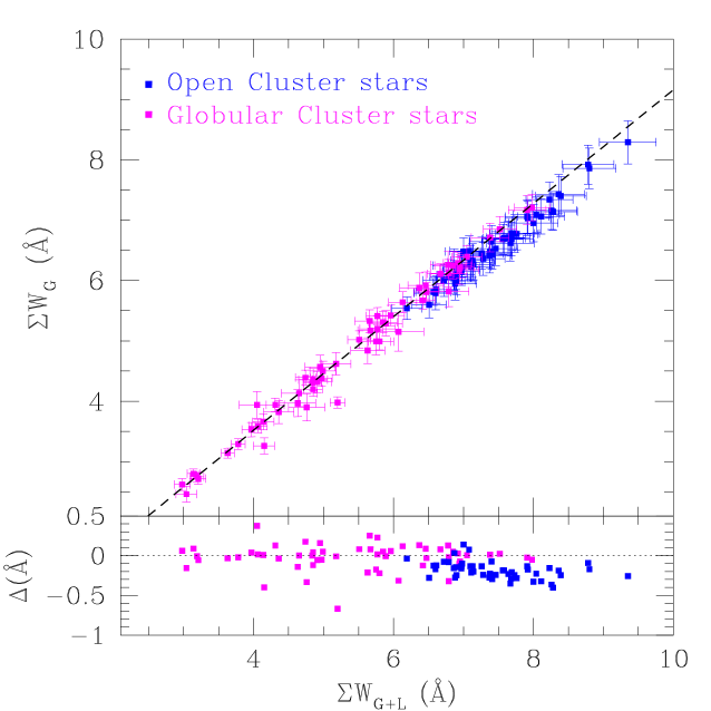
Figure 2: (Top panel) Summed equivalent widths of the 3 CaT lines measured using a Gaussian fit, compared to the same lines fit with the sum of a Gaussian and a Lorentzian function. The dashed line shows the best linear fit to the globular cluster stars. (Bottom panel) The residuals to the fit are plotted, showing how a Gaussian fit increasingly fails to measure the rising fraction of absorption in the far line wings as the lines get stronger.

The composite function fit provides a more satisfactory fit to the line shape, but does it change the resulting equivalent width measurement? We tested the effect of choice of fitting function by remeasuring our targets with the amplitude of the Lorentzian component equal to zero. Figure 2 shows the comparison. The relation between the Gaussian-fit equivalent width, $\Sigma$W_G, and the composite-fit, $\Sigma$W_G+L is linear over much of its range, but there is a change in slope at $\Sigma$W_G+L $\approx$ 6.5 Å. A least-squares fit to the globular cluster stars produces the relation

$$\Sigma W_{G}=0.940\,\Sigma W_{G+L}-0.241,$$ (2)

with r.m.s. scatter of 0.11 Å about the fit for the 57 globular cluster stars. This relation is plotted with a dashed line in the upper panel of Fig. 2. The bottom panel of the figure shows the residuals to this fit, demonstrating that the open cluster stars have similar scatter to the globulars, but are systematically offset by a mean residual of $-$0.2 Å ($\approx$ 2–3%) from the fit. This can be intuitively understood by noting that with increasing line strength, an increasingly larger fraction of the absorption occurs in the line wings, resulting in an ever-larger fraction of absorption missed by the Gaussian fit. The offset corresponds to a difference of 0.05-0.15 dex in the derived metallicities of strong-lined stars.

The “gross underestimation” of the strength of the line wings by a Gaussian fit was already noted by R97a. Because of the increasingly important contribution of the damping wings to the total line width for the strongest lines, we therefore consider only the equivalent widths derived from composite line fits in the remainder of this paper. In the next section, we show that with this choice, the CaT index maintains sensitivity over the range of metallicities considered here. However, the composite fit is noisier than the Gaussian fit because the line depth is small in the far wings. By adding artificial noise to one of our spectra and remeasuring the equivalent widths, we estimate that for signal-to-nosie ratios less than $\approx$ 15–20, there is no significant difference between the two profile shapes. Thus where spectra of low S/N and/or of low metallicity stars are concerned, a fit with fewer free parameters, such as a Moffat function (R97a) may be preferable.

2.4.2 Forming the CaT Index

Metallicity measurements using the CaT index use a linear combination of the three individual Ca II lines to form the line strength index $\Sigma$W (Armandroff & Da Costa, 1991). Various authors have used different procedures to form this index, depending on spectral resolution and signal-to-noise. Some authors have excluded the weakest ($\lambda$ = 8498 Å) line (e.g., Suntzeff et al., 1993; Cole et al., 2000). Others have used all three lines, either weighted (R97a, Smecker-Hane et al., 2003) or unweighted (Olszewski et al., 1991). Because of our extremely high signal-to-noise ratios, we use an unweighted sum of the three lines. The fractional errors on the individal lines are roughly equal, and variations within the sample make it inadvisable to apply a uniform weighting scheme. uniform weighting scheme for all clusters. It has been shown by R97b and Smecker-Hane et al. (2003) that the various means of creating $\Sigma$W produce well-defined linear mappings between the resulting index values. For the remainder of this paper, we adopt the convention

$$\Sigma W\equiv W_{8498}+W_{8542}+W_{8662}.$$ (3)

Stellar effective temperature and surface gravity play a strong role in forming the Ca II lines in red giants, and so the metallicity dependence is typically found using the so-called “reduced” equivalent width (Armandroff & Da Costa, 1991). This quantity is defined as

$$W^{\prime}\equiv\Sigma W+\beta\,(\mathrm{V-V_{HB}}),$$ (4)

where the definition exploits the empirical fact that in an individual globular cluster, all red giants at a given V magnitude have the same $\Sigma$W, and that $\Sigma$W (V) increases linearly up the RGB. V_HB here is the mean magnitude of the horizontal branch; its introduction removes any dependence on the cluster distance or reddening. Other parameterizations for W^′ are possible (e.g., Olszewski et al., 1991), but Equation 4 has the advantages that a huge amount of V band photometry is available in the literature, and that no additional color-dependence is introduced. R97a calibrated Equation 4 using data for 52 Galactic globular clusters and derived a slope $\beta$ = 0.64 $\pm$0.02 Å mag^-1, independently of metallicity, across the range $-$2.1 $\la$ [Fe/H] $\la$ $-$0.6. Consistency with this constant $\beta$ has been found in smaller studies including more metal-rich (open) clusters, such as Melotte 66 (Olszewski et al., 1991), NGC 2477 (Geisler et al., 1995), and M67 (Olszewski et al., 1991; Cole et al., 2000; Smecker-Hane et al., 2003). Defined as in Equation 4, every cluster can be assigned a single value of W^′ that is strongly correlated with metallicity. The relation is linear for the CG97 metallicity scale, but mildly nonlinear for other choices (R97b).

Because we use a different functional form to fit the Ca II lines of our stars, we also need to rederive $\beta$. We did so by deriving the slope for each cluster and taking the average, weighted by the error in the individual values. The resulting slope is $\beta$ = 0.73 $\pm$0.04. This value is higher than found for the globular cluster-only sample of R97a. For reference, the slope determined from our sample of five globulars alone is $\beta_{glob}$ = 0.66 $\pm$0.03, which is indistinguishable from the favored value of R97a, but $<$2$\sigma$ different from our value for all 10 clusters. From the models of Jørgensen et al. (1992), it can be inferred that an increase in $\beta$ with metallicity is in qualitative agreement with theory; direct comparison is difficult because of the interplay between abundance, gravity and temperature and how these quantities vary with age among RGB stars.

The equivalent width measurements for the individual stars are shown in Figure 3, with photometry drawn from the sources listed in Tables 2 & 4. Error bars are omitted so that the best-fitting line (with slope = 0.73) to each cluster can be clearly seen. Note that there is significant scatter about the cluster fiducials even for the well-studied globulars. The mean r.m.s. scatter about each fiducial is $\pm$0.24 Å, larger than our estimated measurement errors; the same effect was found by R97a in their sample. Note that some cluster pairs with metallicities that differ by $\sim$0.1 dex (Melotte 66 and Be 20; NGC 2141 and Be 39) have been plotted using a single point type and fiducial line for clarity. Clusters of such similar abundance are at the limit of our metallicity resolution.

3 Calibrating the Metallicity Scale

Most previous work has found a linear relationship between the reduced equivalent width and [Fe/H] (Armandroff & Da Costa, 1991; Olszewski et al., 1991; Suntzeff et al., 1993; Da Costa & Armandroff, 1995; Geisler et al., 1995; Rutledge et al., 1997b; Cole et al., 2000; Tolstoy et al., 2001; Smecker-Hane et al., 2003; Kraft & Ivans, 2003). The recent standard has been to calibrate to the relation between W^′ and [Fe/H] on the CG97 scale, as given by R97b. Given that we have derived W^′ on a totally different scale from R97b, we will need to rederive this relation.

Figure 4 shows the cluster reduced equivalent widths plotted against the reference abundance on the CG97/F02 scale. The best-fitting line through the data is shown, with the residuals to the fit shown in the bottom panel. The equation of the fit is

$$\mathrm{[Fe/H]^{F02}_{CG97}}=(-2.966\pm 0.032)+(0.362\pm 0.014)\,\mathrm{W^{\prime}},$$ (5)

with r.m.s. scatter $\sigma$ = 0.07 dex. With this set of reference abundances, there is no obvious age effect on the calibration, nor is there any dramatic deviation from the straight-line fit for metallicities beyond the range of the R97b calibration. The only cluster that deviates by as much as 1$\sigma$ from the fit is Be 39; we will discuss the effects of alternate metallicity scales in section 6 below.

Some curvature may be present, based on a predicted loss of CaT index sensitivity at high metallicity (Díaz, Terlevich & Terlevich, 1989). Evidence for just such an effect was presented by Carretta et al. (2001), who were driven primarily by upward revisions of the abundance of the metal-rich bulge globulars NGC 6528 and NGC 6553. If we follow Carretta et al. (2001) in adding a W^′2 term to equation 5, we find the coefficient of the quadratic term to be formally insignificant, and the scatter is not measurably reduced. We conclude that a linear relation suffices to reliably predict [Fe/H] on the currently adopted scale from our measurements of W^′. However, there are two caveats:

1. Homogeneous high-resolution abundances for the open clusters are not yet available, so upward revision of their reference metallicities could change this conclusion.

2. Age-metallicity effects could be conspiring to produce the observed linear relation, i.e., perhaps surface gravity and/or temperature effects cause a variation in W^′ with age that we do not observe because we lack the dynamic range in age at high metallicity to do so.

Both of these points are further discussed below.

4 The Open Cluster Trumpler 5

Trumpler 5 was discovered nearly 75 years go by visual inspection of photographic plates taken by E.E. Barnard in 1894 (Trumpler, 1930). The cluster lies in the Galactic plane $\approx$ 20^∘ from the anticentre, in a region of high and variable interstellar reddening that has complicated attempts to derive its fundamental parameters. Various CMD studies have been undertaken, focusing on the red giant branch in the 1970’s (e.g., Kalinowski et al., 1974), and reaching the unevolved main-sequence in the 1990’s (K98; Kim & Sung, 2003). Authors have converged on values near 3 kpc for the distance, E(B$-$V) = 0.6 for the reddening, and M_V = $-$5.8. K98 recognized that this makes it one of the most massive known open clusters in the Milky Way; we estimate it to be some 5 times as massive as M67, and within a factor of 10 of the massive, intermediate-age clusters of the Magellanic Clouds.

Tr 5 can thus be an important cluster for the study of intermediate-age stellar populations, cluster evolution, and population gradients in the Galaxy. However, no reliable metallicity measurement has yet been made. Kim & Sung (2003) estimate [Fe/H] = $-$0.3 based on the photometry of K98; K98 simply took the metallicity to be equal to that of M67. Because of age-metallicity degeneracy, the age is similarly uncertain; the problem is worsened by the effects of reddening. From the same photometry, K98 and Kim & Sung (2003) derive 4.1 Gyr and 2.4 Gyr, respectively, while the morphological age index of Janes & Phelps (1994) yields 4.9 Gyr.

We included Tr 5 in our observing plans for three reasons: 1) to obtain the first accurate metallicity assessment for this cluster; 2) to make a testable prediction on our calibration of the Ca II triplet method at high metallicities and intermediate ages; and 3) to lay the groundwork for subsequent use of red giants in Tr 5 as metallicity standards for application of the CaT method from 8–10 metre class telescopes (for which nearby clusters are inconveniently bright).

The observed stellar sample towards Tr 5 is given in Table 6, with the adopted V magnitudes, the derived radial velocities, and equivalent widths. No radial velocities have previously been published, so we were unsure whether or not we could reliably discriminate between cluster members and the field. However, we found a well-determined mean heliocentric radial velocity V_r = $+$54 $\pm$5 km sec^-1, where the uncertainty reflects the r.m.s. scatter of the member stars about the mean. This squarely assigns Tr 5 to the Galactic disc, but it may be lagging in rotation by 10–20 km sec^-1 compared to the thin disc– which is unsurprising, given its estimated age.

Two stars were excluded from further analysis based on their blueshifts of 40 and 60 km sec^-1 respectively relative to the cluster– consistent with them being dwarfs in the solar neighborhood. We initially chose our stars based on the 2MASS (K_S, J$-$K_S) CMD, but later inspection of the K98 (V, B$-$V) data showed that three of the stars in the southern part of the cluster appeared to be differentially reddened away from the main cluster RGB; these stars are identified and excluded from further analysis. Two of the stars near the observed tip of the red giant branch were treated with care because the cluster is known to harbor M giants, for which TiO veiling can bias the CaT-derived metallicities (Olszewski et al., 1991). However, any TiO bands must be weak, or they would have been obvious in our spectra. We decided to include the 2 possible early M stars because they don’t significantly change the cluster metallicity, so any continuum veiling bias must be small.

The equivalent widths and magnitudes of the ten remaining RGB stars are shown in Figure 5. From these measurements and Equation 5 we derive the metallicity of Trumpler 5 [Fe/H] = $-$0.56 $\pm$0.11. Lines corresponding to this value and range are shown in the figure. This is lower than the metallicities estimated from the K98 CMDs, but consistent with its large galactocentric radius ($\approx$ 11 kpc). A full re-analysis of the CMDs is beyond the scope of this paper, but we use isochrones from Girardi et al. (2000) interpolated to the correct metallicity to rederive the cluster age. Using the VI data, we find good agreement with the main-sequence, subgiant branch, and lower RGB for a distance of 2.8 kpc, a reddening E(B$-$V) = 0.66 mag, and an age of 3.0 $\pm$0.5 Gyr. The age is between the values reported by K98 and Kim & Sung (2003), for 10–14% higher reddening and 7–18% smaller distance.

Kalinowski et al. (1974) observed that the carbon star V493 Mon is projected within 2$\aas@@fstack{\prime}$5 of the cluster centre and has typical optical magnitudes for an N-type C star if assumed to lie at the cluster distance and reddening. This is also true if one considers the near-infrared photometry from Iijima & Ishida (1978). Assigning a membership probability will require precise radial velocities and proper motions; however, a highly discrepant radial velocity is sufficient to rule out membership. We find V_r = $+$46 km sec^-1, close to the cluster mean. Considering its projected distance within 1/4 of the cluster radius of the centre, the surface density of field carbon stars, the optical photometry, the infrared photometry, and the radial velocity, V493 Mon seems to be a more than likely member of Trumpler 5.

5 Application to Composite Populations

The CaT method is the best available route to metallicity measurements of RGB stars in nearby galaxies (e.g., Suntzeff et al., 1993; Tolstoy et al., 2001). There are two potential difficulties in its application. First, the reduced equivalent width, and its correlation with [Fe/H], are only defined and calibrated to stars older than $\sim$10 Gyr and more metal-poor than $\sim\frac{1}{3}$ solar. While this does not present severe problems for some of the smallest dwarf spheroidals (Draco, Ursa Minor, Tucana), most Local Group galaxies contain substantial populations that violate either the age or metallicity range of the R97b calibration (Mateo, 1998). We have begun to address this calibration issue with these data.

Second, star clusters give a strongly biased view of the star-formation history of a galaxy, so the field stars are of primary interest. Yet in a composite sample, the unknown mixture of ages and metallicities makes it impossible to assign a unique horizontal branch magnitude that is to be used in the abundance determination of an individual star. The observed horizontal branch (or more generally, red clump) is more extended in the field than the cluster, because of the variation of clump magnitude with age and metallicity (e.g., Cole, 1998; Girardi & Salaris, 2001).

A first approach to this problem was made by Da Costa & Hatzidimitriou (1998) in their study of SMC clusters. These authors measured the mean red clump magnitude in each cluster to create their reduced equivalent widths, and then applied a theoretically-derived correction factor to the metallicity, based on the variation of clump magnitude with age. The corrections were of order $-$0.05 dex for the age range from 3.5–10 Gyr, smaller than the precision of the abundances. We dispense with this type of correction here, because we have included younger clusters in our calibrations, and the variation of their red clump magnitude is thus folded into Equation 5.

Cole et al. (2000) estimated the bias introduced by the use of a composite V_HB in the calculation of W^′ for field stars, and found similar results to Da Costa & Hatzidimitriou (1998). We make a new, empirical measurement of the bias without recourse to theoretical models by considering all of our star clusters together (“mixed”), rather than individually (“unmixed”). We do this by shifting each cluster to a common apparent distance modulus (m$-$M)_V, and calculating the mean horizontal branch magnitude of the mixed population, $\langle{\mathrm{M}_{V}}\rangle=0.63$, with an r.m.s. scatter of 0.14 mag. Using new values of V$-$V_HB calculated with this mean HB magnitude, we recomputed the metallicities of each cluster.

The result of this exercise is shown in Figure 6. The difference between the mixed vs. the unmixed metallicities is plotted against the unmixed metallicities for the individual stars in each cluster. Since the difference is constant within a cluster, the clusters spread out along horizontal lines in this plot. The errorbars in the $y$-coordinate give the r.m.s. spread in metallicity of each cluster. Figure 6 clearly shows that the bias introduced by variation of horizontal branch/red clump magnitude with age is smaller than the intrinsic precision of the method. At low abundances, a trend with metallicity is apparent, but at the high end of the range, the effect is not clear, perhaps due to errors in the distances of the clusters, or perhaps due to a complicated interaction between age and metallicity effects. Figure 6 is empirically supportive of the theoretically-motivated corrections suggested by Da Costa & Hatzidimitriou (1998) and Cole et al. (2000). The small size of the offsets indicates that application of the CaT method to field populations of mixed age and metallicity does not introduce large biases in the derived metallicities, within the range of parameters considered here.

6 Summary & Discussion

In connexion with a programme to determine the age-metallicity relation and radial abundance gradient of field red giants in the LMC (Cole et al., 2000; Smecker-Hane et al., 2003, Cole et al. 2003 in preparation), we have obtained medium-resolution spectra of red giants in 11 Galactic star clusters at the near-infrared Ca II triplet (CaT) using the FORS2 multiobject spectrograph at the 8.2-metre VLT/UT4. Our spectra have extremely high signal-to-noise, ranging from 20 $\leq$ S/N $\leq$ 85. Following many previous authors (e.g., R97b) we have derived a linear relation between the equivalent width of the CaT and the cluster metallicities.

For the first time, our sample includes open clusters with a range of metallicities from $-$0.6 $\la$ [Fe/H] $\la$ $-$0.2 and ages from 2.5 $\la$ (age/Gyr) $\la$ 7. This allows an initial assessment of the effects of age on the metallicity measurement via the CaT. While there is is substantial scatter and the sample size is small, we find no evidence for a decrease in sensitivity of the CaT at young ages and high metallicities. This behavior is theoretically supported by non-LTE stellar atmosphere calculations (e.g., Jørgensen et al., 1992) and is in good agreement with comprehensive empirical calibrations of the CaT behavior over a wide range of stellar atmospheric parameters (e.g., Cenarro et al., 2002). However, our results disagree with earlier results based on more limited stellar samples (e.g., Jones, Alloin & Jones, 1984; Carter, Visnavathan & Pickles, 1986; Díaz, Terlevich & Terlevich, 1989). The fact that we see no loss of metallicity sensitivity above [Fe/H] $\approx$ $-$0.5 is interesting in light of the observed metallicity independence of calcium line strength in the integrated light of clusters and galaxies above this level (e.g., Vazdekis et al., 2003).

One difference between our analysis and earlier work is that we fit a composite function– the sum of a Gaussian and a Lorentzian– to the line profiles. This is mandated by the line shapes, which indicate that for abundance [Fe/H] $\ga$ $-$0.6, the damping wings of the lines are so strong and broad that we begin to resolve the line even at our resolution of $\sim$2.5 Å.

Using our data, we obtain a linear relation between the reduced equivalent width of a cluster, W^′, and metallicity on a scale formed by the high-dispersion results of CG97 for the globular clusters, and medium-dispersion Fe indices from F02 for the open clusters. There is no indication that a second-order term in W^′, as advocated by Carretta et al. (2001), is needed to fit the data. However, our sample does not include old, high-metallicity clusters (such as bulge globulars NGC 6528 and NGC 6553), clusters of supersolar metallicity (such as NGC 6791 and NGC 6253), or young clusters of very low abundance (such as the clusters of the Small Magellanic Cloud). Until such time as the age-metallicity plane is filled, we cannot definitively rule out an age effect on the calibration. Filling in the high-metallicity regime at a large range of ages will have important consequences for the determination of abundances in the M31 halo.

An important point is that the globular cluster metallicity scale is not absolutely established. The CG97 scale differs in a nonlinear way from the average of spectrophotometric indices compiled by Zinn & West (1984). In turn, CG97 may be superseded by abundance scales derived from Fe II lines, rather than Fe I lines, because of the newly-recognized importance of non-LTE effects (Kraft & Ivans, 2003). The open cluster abundances are even more uncertain, and will remain so until large-scale, homogeneous surveys for high-dispersion spectra can be undertaken. This type of analysis is presently available for only a small number of stars in a small number of clusters; among our sample, Melotte 66 and M67 have been analyzed. Photometric metallicity indicators based on DDO-system or Strömgren photometry (e.g., Twarog et al., 1997) often give quite different results from the indices tabulated by Friel and collaborators. The choice of metallicity scales will of course have a strong effect on the calibration of the CaT. We tabulate some alternate cluster metallicities in Table 8. Columns 1–4 give the cluster name, W^′ derived from Equation 4, the reference abundance from Table 1, and the derived metallicity using Equation 5. Alternate metallicities are given in column 5, sorted by origin, and referenced in the last column. Using the tabulated values of W^′ and [Fe/H]_alt, we derive the following relation (excluding Tr 5):

$$\mathrm{[Fe/H]_{alt}}=-2.629\,+0.058\,\mathrm{W^{\prime}}\,+0.037\,\mathrm{W^{\prime 2}}.$$ (6)

Significant curvature is introduced into the relationship because the globular cluster metallicities have been shifted down, while the open cluster metallicities, especially NGC 2141 and M67, have been shifted upwards. The cluster metallicities derived from Equation 6 are given in Table 8. We cannot comment on the correct choice of metallicity scales, but we note that although the linearity of the CaT calibration seems to be a fortuitous result of one such choice, the one-to-one correspondance between W^′ and [Fe/H] holds no matter the choice of reference metallicities (as already noted by Kraft & Ivans, 2003).

We have measured the bias introduced by taking the mean horizontal branch/red clump magnitude of a composite field population in determining the quantity V$-$V_HB. Shifting all 10 clusters to a common apparent distance modulus and taking the mean V_HB of the mixed population results in derived metallicities that shift by $\pm$0.05 dex relative to the unmixed results. This is negligible within the uncertainties, and shows that measurements of individual field red giants yield reliable metallicities despite the lack of a unique V_HB in that scenario– although the additional uncertainty should be considered in the error analyses. The mixed-population bias is clearly not random at the low-metallicity end of our calibration sample, where the age range is small. This is consistent with theoretical expectations for the variation of V_HB with metallicity (e.g., Girardi & Salaris, 2001). At the high-metallicity end, the picture becomes more complicated, with age and abundance effects combining with distance uncertainties to introduce additional scatter.

We have made the first measurement of the metallicity of the large, old open cluster Trumpler 5, finding [Fe/H] = $-$0.56 $\pm$0.11. While interesting in itself, this also represents a testable prediction of our calibration of the CaT. With our metallicity estimate, the most likely age for Tr 5 is 3.0 $\pm$0.5 Gyr. The relatively low metallicity of Tr 5 places the cluster in a category with objects such as Melotte 66. It somewhat diminishes the utility of Tr 5 as an intermediate-age, high-metallicity calibrator for the Ca II triplet, but makes it easier to theoretically understand the possible presence of a carbon star in the cluster. The carbon star, V493 Mon, has a radial velocity within 8 km sec^-1 of the cluster mean. Given the large number of independent data consistent with membership, it would be surprising if V493 Mon turned out to be a field interloper. However, more precise velocities, as well as proper motions, are needed to assign V493 Mon to Tr 5 for certain. This raises the exciting possibility that detailed study of the cluster will yield its turnoff mass ($\approx$ 1.14${}^{+0.09}_{-0.04}$ M_☉), and therefore a direct measurement of the mass of the progenitor of an intermediate-mass, moderate-metallicity carbon star.

We are further refining the empirical calibration of the CaT by enlarging the sample of high-metallicity, intermediate-age cluster giants with high signal-to-noise spectra. TLB and TSH have measured the spectra of numerous giants in several clusters, at both high- and low-dispersion, using the Shane 3-metre Telescope at Lick Observatory. The cluster sample spans the abundance range from $-$2.3 $\leq$ [Fe/H] $\leq$ $+$0.4 and ages $\ga$ 2 Gyr. In addition to the new CaT measurements, we will determine [Ca/H] abundances for the clusters using model atmosphere analyses of the strengths of the plentiful neutral calcium lines (which are theoretically much better understood) in the high-dispersion spectra. We will calibrate the relationship between the CaT index and [Ca/H], eliminating the need to assume a specific [Ca/Fe] vs. [Fe/H] relationship. This is an important step for application of the CaT technique across diverse environments which may have experienced very different histories of chemical evolution (e.g., dwarf galaxies Tolstoy et al., 2003).

Our results are a striking reaffirmation of the utility of the CaT for abundance measurements of red giants in intermediate-age field populations. Red giants are the brightest common stars among old stellar populations, and so they are currently the only practical targets for abundance analyses of stars aged $\approx$ 2–14 Gyr in Local Group galaxies beyond the Milky Way halo. In these systems, the typical magnitude of the RGB tip is I $\ga$ 20, and measurement of the CaT from low-resolution spectra is the most direct available method to accrue the large samples of abundance measurements needed to assess the chemical evolution of systems beyond the Milky Way halo.

Table 1: The Cluster Sample

Cluster	$\alpha$ (J2000)	$\delta$ (J2000)	[Fe/H]	Age (Gyr)	(m$-$M)V	VHB	Reference
NGC 104 (47 Tuc)	00:26:33	$-$71:51	$-$0.70 $\pm$0.07	10.7	13.37	14.06	1,2,3
NGC 1851	05:14:15	$-$40:04	$-$0.98 $\pm$0.06	9.2	15.47	16.09	2,3,4
NGC 1904 (M79)	05:24:12	$-$24:31	$-$1.37 $\pm$0.01	11.7	15.59	16.15	1,2,3
NGC 2298	06:48:59	$-$36:00	$-$1.74 $\pm$0.06	12.6	15.59	16.11	1,2,3
NGC 4590 (M68)	12:39:28	$-$26:45	$-$1.99 $\pm$0.10	11.2	15.19	15.68	1,2,3
Berkeley 20	05:32:34	$+$00:10	$-$0.61 $\pm$0.14	4.9	15.01	15.70	5,6
NGC 2141	06:03:00	$+$10:30	$-$0.33 $\pm$0.10	2.8	14.16	14.90	5,7
Melotte 66	07:26:28	$-$47:41	$-$0.47 $\pm$0.09	6.3	13.63	14.52	5,8
Berkeley 39	07:46:45	$-$04:41	$-$0.26 $\pm$0.09	7.2	13.78	14.28	5,8
NGC 2682 (M67)	08:51:25	$+$11:48	$-$0.15 $\pm$0.05	6.3	9.98	10.54	5,8
Trumpler 5	06:36:34	$+$09:27	$-$0.3:	4 :	14.40	15.13	9,10

References to metallicity, distance modulus, and V_HB values: (1) Carretta & Gratton (1997); (2) Salaris & Weiss (2002); (3) Harris (1996); (4) Rutledge et al. (1997b); (5) Friel et al. (2002); (6) MacMinn et al. (1994); (7) Rosvick (1995); (8) Sarajedini (1999); (9) Kałuzny (1998); (10) Kim & Sung (2003).

Table 2: Observed Stars: Globular Clusters

Star	V	Vr (km s-1)	$\Sigma$W (Å)
47 Tuc: Lee (1977)
L5309	12.21	-21.8 $\pm$7.6	7.98 $\pm$0.10
L5310‡	13.41	9.1 $\pm$7.6	6.46 $\pm$0.10
L5312	12.18	-12.3 $\pm$7.5	7.91 $\pm$0.10
L5418	15.33	-20.6 $\pm$7.9	5.77 $\pm$0.16
L5419	14.05	-22.2 $\pm$7.8	6.13 $\pm$0.12
L5422	12.47	-23.1 $\pm$7.6	7.38 $\pm$0.10
L5527	13.56	-25.5 $\pm$7.6	6.79 $\pm$0.09
L5528	14.40	-28.5 $\pm$7.6	6.37 $\pm$0.18
L5530	13.14	-18.6 $\pm$7.6	6.92 $\pm$0.08
‡ Radial velocity nonmember, excluded from analysis.
NGC 1851: Stetson (1981)
003	13.60	324.5 $\pm$7.4	7.52 $\pm$0.15
065	15.75	322.1 $\pm$7.5	5.67 $\pm$0.08
095	13.57	334.1 $\pm$7.4	6.94 $\pm$0.11
107	14.50	330.7 $\pm$7.5	6.78 $\pm$0.13
109	14.85	334.3 $\pm$7.4	5.96 $\pm$0.10
112	13.80	327.3 $\pm$7.4	6.85 $\pm$0.11
123	16.21	329.7 $\pm$7.4	4.99 $\pm$0.08
126	14.29	321.5 $\pm$7.5	6.95 $\pm$0.11
160	15.51	326.4 $\pm$7.7	5.85 $\pm$0.09
175	16.22	332.3 $\pm$7.9	6.07 $\pm$0.10
179	16.45	320.4 $\pm$7.8	5.66 $\pm$0.08
195	15.82	327.6 $\pm$7.5	5.75 $\pm$0.09
209	14.08	333.4 $\pm$7.6	7.05 $\pm$0.20
231	15.93	332.8 $\pm$7.8	5.89 $\pm$0.10
275	14.98	333.8 $\pm$7.6	6.79 $\pm$0.13
NGC 1904: Stetson & Harris (1977)
006	15.27	203.2 $\pm$7.4	4.91 $\pm$0.08
011	15.74	213.5 $\pm$7.5	4.85 $\pm$0.10
015	13.22	204.8 $\pm$7.5	6.67 $\pm$0.10
045	15.58	206.8 $\pm$7.8	4.95 $\pm$0.08
089	14.71	206.5 $\pm$7.8	5.51 $\pm$0.09
091	16.25	207.6 $\pm$7.8	4.76 $\pm$0.08
111	15.62	206.9 $\pm$7.6	5.18 $\pm$0.08
115	15.95	211.0 $\pm$7.7	4.65 $\pm$0.10
138	16.16	206.3 $\pm$7.8	4.36 $\pm$0.08
153	13.44	206.1 $\pm$7.4	6.47 $\pm$0.11
160	13.02	200.3 $\pm$7.5	6.42 $\pm$0.10
161	15.86	216.5 $\pm$7.8	4.05 $\pm$0.07
176	14.95	215.9 $\pm$7.6	4.74 $\pm$0.08
209	15.02	210.8 $\pm$7.5	5.63 $\pm$0.11
224	16.09	220.4 $\pm$7.9	4.63 $\pm$0.09
237	14.19	220.8 $\pm$7.5	5.77 $\pm$0.11
241	13.61	228.5 $\pm$7.5	5.80 $\pm$0.09

Table 3: continued

Observed Stars: Globular Clusters Star V V_r (km s^-1) $\Sigma$W (Å) NGC 2298: Alcaino & Liller (1986) 6 13.82 156.5 $\pm$7.6 4.97 $\pm$0.07 12 14.23 146.6 $\pm$7.5 4.84 $\pm$0.07 15 14.86 151.2 $\pm$7.6 4.31 $\pm$0.06 22 15.30 162.0 $\pm$7.4 4.06 $\pm$0.06 25 15.69 153.2 $\pm$7.5 4.15 $\pm$0.06 S156^⋆ 15.53 148.5 $\pm$7.6 4.14 $\pm$0.05 S172^⋆ 15.61 160.6 $\pm$7.7 3.97 $\pm$0.05 ^⋆ ID and magnitude from T. Smecker-Hane, unpublished. NGC 4590: Harris (1975) I-2 14.95 -96.0 $\pm$7.6 2.98 $\pm$0.04 I-49 14.62 -93.6 $\pm$7.8 3.04 $\pm$0.05 I-74 14.59 -103.7 $\pm$7.7 3.21 $\pm$0.05 I-119 13.62 -89.1 $\pm$7.6 3.78 $\pm$0.06 I-239 14.19 -86.0 $\pm$7.6 3.63 $\pm$0.05 I-256 12.64 -90.9 $\pm$7.6 5.20 $\pm$0.08 I-258 14.24 -90.2 $\pm$7.7 3.14 $\pm$0.05 I-260 12.52 -91.4 $\pm$7.5 4.85 $\pm$0.07 II-47 15.03 -85.8 $\pm$7.8 3.19 $\pm$0.05

Table 4: Observed Stars: Open Clusters

Star	V	Vr (km s-1)	$\Sigma$W (Å)
Berkeley 20: MacMinn et al. (1994)
05	14.80	73.9 $\pm$7.5	7.56 $\pm$0.12
08	15.15	79.2 $\pm$7.5	7.41 $\pm$0.12
12	16.21	83.8 $\pm$7.5	6.61 $\pm$0.12
22	16.90	74.6 $\pm$7.5	6.19 $\pm$0.13
29‡	17.14	42.1 $\pm$7.7	5.52 $\pm$0.17
‡ Radial velocity nonmember, excluded from analysis.
NGC 2141: Burkhead, Burgess & Haisch (1972); Rosvick (1995)
1-3-21	14.18	31.8 $\pm$7.5	8.04 $\pm$0.18
1-4-05	14.61	50.7 $\pm$7.5	7.58 $\pm$0.13
3-2-18	13.05	26.0 $\pm$7.5	9.35 $\pm$0.18
3-2-34	14.95	27.6 $\pm$7.5	7.26 $\pm$0.17
3-2-40	13.25	28.9 $\pm$7.4	8.80 $\pm$0.17
3-2-52	14.36	33.2 $\pm$7.5	7.67 $\pm$0.14
3-2-56‡	15.54	-11.3 $\pm$7.5	4.15 $\pm$0.09
4-08	14.80	23.2 $\pm$7.6	7.76 $\pm$0.13
4-09	13.27	28.7 $\pm$7.6	8.78 $\pm$0.14
4-13	15.15	32.1 $\pm$7.4	6.79 $\pm$0.14
4-14	15.52	28.8 $\pm$7.4	7.38 $\pm$0.12
4-24	14.77	31.4 $\pm$7.5	7.64 $\pm$0.13
4-25	14.13	31.3 $\pm$7.5	8.11 $\pm$0.18
5-09	14.62	33.0 $\pm$7.5	7.69 $\pm$0.14
5-13	13.96	32.0 $\pm$7.5	7.92 $\pm$0.15
5-13a	15.00	49.3 $\pm$7.4	7.00 $\pm$0.16
‡ Radial velocity nonmember, excluded from analysis.
Melotte 66: Anthony-Twarog, Twarog & McClure (1979)
1205	14.18	18.3 $\pm$7.5	6.86 $\pm$0.11
2107	14.70	14.9 $\pm$7.5	6.57 $\pm$0.11
2133	13.20	10.9 $\pm$7.5	7.91 $\pm$0.12
2226	14.08	18.9 $\pm$7.5	7.11 $\pm$0.19
2233	15.44	14.4 $\pm$7.4	6.51 $\pm$0.09
2244	14.47	16.4 $\pm$7.6	6.97 $\pm$0.09
2261	13.64	41.2 $\pm$7.5	7.46 $\pm$0.16
3101	14.98	15.6 $\pm$7.7	5.03 $\pm$0.10
3133	14.08	17.2 $\pm$7.6	6.98 $\pm$0.12
3229	13.93	7.7 $\pm$7.5	7.08 $\pm$0.31
3235	14.66	18.3 $\pm$7.7	6.89 $\pm$0.10
3260	14.56	16.2 $\pm$7.4	6.90 $\pm$0.12
4151	12.69	12.7 $\pm$7.6	8.23 $\pm$0.13
4265	14.07	7.4 $\pm$7.5	6.97 $\pm$0.12

Table 5: continued

Observed Stars: Open Clusters Star V V_r (km s^-1) $\Sigma$W (Å) Berkeley 39: Kałuzny & Richtler (1989) 002 13.09 56.5 $\pm$7.5 8.39 $\pm$0.18 003 13.55 61.0 $\pm$7.4 8.26 $\pm$0.18 005 13.88 56.5 $\pm$7.5 7.68 $\pm$0.16 009 14.23 56.7 $\pm$7.5 7.14 $\pm$0.13 012 14.34 55.9 $\pm$7.4 7.37 $\pm$0.14 013 14.35 58.2 $\pm$7.5 6.87 $\pm$0.16 016 14.48 61.4 $\pm$7.5 7.28 $\pm$0.15 017 14.75 54.0 $\pm$7.6 6.72 $\pm$0.12 018 14.76 57.9 $\pm$7.5 6.88 $\pm$0.14 028 15.40 58.9 $\pm$7.5 6.60 $\pm$0.15 M67^⋆: Johnson & Sandage (1955); Sanders (1977) F104 11.20 33.5 7.13 $\pm$0.16 F105 10.30 34.3 8.00 $\pm$0.16 F108 9.72 34.7 8.36 $\pm$0.17 F135 11.44 34.3 7.10 $\pm$0.13 F141 10.48 33.6 7.73 $\pm$0.14 F164 10.55 33.3 7.40 $\pm$0.15 F170 9.69 34.3 8.28 $\pm$0.19 1264^§ 11.74 34.9 5.83 $\pm$0.23 ^⋆ Radial velocities from Mathieu et al. (1986). ^§ Blend (Montgomery, Marschall & Janes, 1993); excluded from analysis.

Table 6: Observed Stars: Trumpler 5

Star†	V (mag)	Vr (km s-1)	$\Sigma$W (Å)	Note
K3763	14.54	-3.9 $\pm$7.5	7.71 $\pm$0.03	1
K3354	14.48	53.7 $\pm$7.5	6.85 $\pm$0.02
K3066	14.39	50.7 $\pm$7.4	7.04 $\pm$0.03
K2579	15.59	47.8 $\pm$7.5	6.37 $\pm$0.03
K2565	15.79	60.5 $\pm$7.5	6.12 $\pm$0.03
K2324	15.03	53.1 $\pm$7.5	6.70 $\pm$0.02
K2280	15.16	47.8 $\pm$7.4	6.54 $\pm$0.03
K1935	12.87	53.5 $\pm$7.5	8.63 $\pm$0.03	2
K1834	16.24	50.8 $\pm$7.7	6.21 $\pm$0.05
K1401	15.29	14.8 $\pm$7.5	6.60 $\pm$0.03	1
K1305	14.24	64.9 $\pm$7.5	8.12 $\pm$0.03	3
K1277	14.92	46.3 $\pm$7.2		4
K1214	13.91	55.7 $\pm$7.5	7.61 $\pm$0.03	2
K1026	14.73	52.0 $\pm$7.3	6.48 $\pm$0.10
K833	14.91	54.4 $\pm$7.4	6.53 $\pm$0.04	3
K488	16.51	57.1 $\pm$7.7	7.31 $\pm$0.05	3

^† From Table 3 of Kałuzny (1998).
Notes: (1) radial velocity nonmember; (2) weak TiO?; (3) Probably differentially reddened; (4) Carbon star $\equiv$ V493 Mon.

Table 7: Cluster Radial Velocities

	Vr	$\sigma$(Vr)	prev. Vr
Cluster	(km s-1)	(km s-1)	(km s-1)	Reference
47 Tuc	$-$22	5	$-$18.7	1
NGC 1851	329	5	320.5	1
NGC 1904	211	7	206.0	1
NGC 2298	154	6	148.9	1
NGC 4590	$-$92	6	$-$94.3	1
Be 20	78	5	70	2
NGC 2141	33	5	64	3
Mel 66	16	8	23	4
Be 39	58	2	55	2
M67			33	2
Tr 5	54	5

References: (1) Harris (1996); (2) Friel et al. (2002); (3) Friel, Liu, & Janes (1989); (4) Friel & Janes (1993).

Table 8: Cluster Metallicity Data

	W′	[Fe/H]	[Fe/H]	[Fe/H]†	[Fe/H]
Cluster	(Å)	(ref)	(Eqn. 5)	(alt.)	(Eqn. 6)	Reference
47 Tuc	6.36 $\pm$0.03	$-$0.70 $\pm$0.07	$-$0.66 $\pm$0.09	$-$0.88, $-$0.71	$-$0.77 $\pm$0.13	1,2
NGC 1851	5.55 $\pm$0.02	$-$0.98 $\pm$0.06	$-$0.96 $\pm$0.12	$-$1.19, $-$1.33	$-$1.17 $\pm$0.16	1,2
NGC 1904	4.40 $\pm$0.02	$-$1.37 $\pm$0.01	$-$1.37 $\pm$0.11	$-$1.64, $-$1.68	$-$1.66 $\pm$0.12	1,2
NGC 2298	3.54 $\pm$0.03	$-$1.74 $\pm$0.06	$-$1.69 $\pm$0.07	$-$2.07, $-$1.81	$-$1.96 $\pm$0.06	1,2
NGC 4590	2.48 $\pm$0.03	$-$1.99 $\pm$0.10	$-$2.07 $\pm$0.09	$-$2.43, $-$2.09	$-$2.25 $\pm$0.26	1,2
Be 20	6.91 $\pm$0.03	$-$0.61 $\pm$0.14	$-$0.47 $\pm$0.07	$-$0.4	$-$0.47 $\pm$0.11	3
NGC 2141	7.47 $\pm$0.02	$-$0.33 $\pm$0.10	$-$0.26 $\pm$0.10	$-$0.06	$-$0.14 $\pm$0.16	4
Mel 66	6.86 $\pm$0.03	$-$0.47 $\pm$0.09	$-$0.48 $\pm$0.06	$-$0.38, $-$0.35	$-$0.50 $\pm$0.10	5,4
Be 39	7.32 $\pm$0.03	$-$0.26 $\pm$0.09	$-$0.32 $\pm$0.09	$-$0.18	$-$0.24 $\pm$0.14	4
M67	7.68 $\pm$0.06	$-$0.15 $\pm$0.05	$-$0.19 $\pm$0.05	$-$0.05, 0.00	$-$0.01 $\pm$0.09	6,4
Tr 5	6.63 $\pm$0.03		$-$0.56 $\pm$0.11	$-$0.3	$-$0.62 $\pm$0.14	7

^† Values in roman type are from high-dispersion spectroscopy; values in italic type are from photometric or spectrophotometric indices.
References: (1) Kraft & Ivans (2003); (2) Zinn & West (1984); (3) Durgapal et al. (2001); (4) Twarog et al. (1997); (5) Gratton & Contarini (1994); (6) Shetrone & Sandquist (2000); (7) Kim & Sung (2003).

Figure 1: Sample spectra for stars in three clusters, representative of the range of line strengths in our targets. The spectra have been sky-subtracted, continuum-normalized, and Doppler-shifted to the rest frame for comparison. Each spectrum is offset by a constant amount from the one below. Stars are identified by cluster name and metallicity from Table 1, and ID from Tables 2 and 4. Most of the “noise” in the most metal-rich spectrum is due to the increasing strength of a large number of relatively weak atomic lines, mainly Fe I.

Figure 3: The CaT equivalent widths of RGB stars in 10 star clusters compared to their magnitude above their respective cluster horizontal branches. The solid lines show the best-fitting lines to each cluster, assuming the best common slope of 0.73 Å mag^-1. Clusters are represented by: closed squares (NGC 4590), open squares (NGC 2298), closed triangles (NGC 1904), open triangles (NGC 1851), crosses (47 Tuc), stars (Mel 66 and Be 20), open circles (NGC 2141 and Be 39), and closed circles (M67). The fit to NGC 4590 adopting the slope from R97a of 0.64 Å mag^-1 is shown for comparison (dotted line). Errorbars are omitted for clarity, but the typical 1$\sigma$ errors are shown at lower left.

Figure 4: (Top panel) The reference metallicity of the 10 clusters in Table 1 plotted against their reduced CaT equivalent width. The best linear fit to the data is shown. (Bottom panel) the residuals to the linear fit are plotted; the errorbars are 1$\sigma$ errors on the reference abundance.

Figure 5: CaT equivalent widths vs. V magnitude for 10 RGB stars in the old open cluster Trumpler 5. The lines corresponding to the best-fitting metallicity according to our calibration (solid), and the formal 1$\sigma$ rms scatter (dashed) are shown, with reference lines (dotted) corresponding to $-$0.2 and $-$1.0 dex.

Figure 6: The difference between “mixed” and “unmixed” abundance estimates for the 10 well-studied star clusters. The “mixed” estimates are made by shifting all clusters to a common (m$-$M)_V and using the combined average red clump $+$ horizontal branch magnitude to define V_HB. The errorbars show the rms scatter of the “unmixed” abundances of each cluster.

References

- Alcaino & Liller (1986) Alcaino G., Liller W., 1986, A&A, 161, 61
- Alonso et al. (1999) Alonso A., Arribas S., Martìnez-Roger C., 1999, A&A, 140, 261
- Anthony-Twarog, Twarog & McClure (1979) Anthony-Twarog B.J., Twarog B.A., McClure R.D., 1979, ApJ, 233, 188
- Armandroff & Da Costa (1991) Armandroff T.E., Da Costa G.S., 1991, AJ, 101, 1329
- Armandroff & Zinn (1988) Armandroff T.E., Zinn, R., 1988, AJ, 96, 92
- Burkhead, Burgess & Haisch (1972) Burkhead M.S., Burgess R.D., Haisch B.M., 1972, AJ, 77, 661
- Butcher (1977) Butcher H., 1977, ApJ, 216, 372
- Carretta & Gratton (1997) Carretta E., Gratton R.G., 1997, A&AS, 121, 95
- Carretta et al. (2001) Carretta E., Cohen J.G., Gratton R.G., Behr B.B., 2001, AJ, 122, 1469
- Carter et al. (1986) Carter D., Visnavathan N., Pickles A.J., 1986, ApJ, 311, 637
- Cenarro et al. (2001a) Cenarro A.J., Cardiel N., Gorgas J., Peletier R.F., Vazdekis A., Prada F., 2001a, MNRAS, 326, 959
- Cenarro et al. (2002) Cenarro A.J., Gorgas J., Cardiel N., Vazdekis A., Peletier R.F., 2002, MNRAS, 329, 863
- Cole (1998) Cole A.A., 1998, ApJL, 500, L137
- Cole et al. (2000) Cole A.A., Smecker-Hane T.A., Gallagher J.S., 2000, AJ, 120, 1808
- Cottrell & Sneden (1986) Cottrell P.L., Sneden C., 1986, A&A, 161, 314
- Da Costa & Armandroff (1995) Da Costa G.S., Armandroff T.E., 1995, AJ, 109, 2533
- Da Costa & Hatzidimitriou (1998) Da Costa G.S., Hatzidimitriou D., 1998, AJ, 115, 1934
- Díaz et al. (1989) Díaz A.I., Terlevich E., Terlevich R., 1989, MNRAS, 239, 325
- Durgapal et al. (2001) Durgapal A.K., Pandey A.K., Mohan V., 2001, A&A, 372, 71
- Friel & Janes (1993) Friel E.D., Janes K.A., 1993, A&A, 267, 75
- Friel et al. (1989) Friel E.D., Liu T., Janes K.A., 1989, PASP, 101, 1105
- Friel et al. (2002) Friel E.D., Janes K.A., Tavarez M., Scott J., Katsanis R., Lotz J., Hong L., Miller N., 2002, AJ, 124, 2693 (F02)
- Geisler et al. (1995) Geisler D., Piatti A.E., Clariá J.J., Minniti D., 1995, AJ, 109, 605
- Girardi & Salaris (2001) Girardi L., Salaris M., 2001, MNRAS, 323, 109
- Girardi et al. (2000) Girardi L., Bressan A., Bertelli G., Chiosi C., 2000, A&AS, 141, 371
- Gratton & Contarini (1994) Gratton R.G., & Contarini G., 1994, A&A, 283, 911
- Gustafsson et al. (1975) Gustafsson B.E., Bell R.A., Eriksson K., Nordlund A., 1975, A&A, 42, 407
- Harris (1975) Harris W.E., 1975, ApJS, 29, 397
- Harris (1996) Harris W.E., 1996, AJ, 112, 1487
- Hill et al. (2000) Hill V., François P., Spite M., Primas F., Spite F., 2000, A&A, 364, L19
- Iijima & Ishida (1978) Iijima T., Ishida K., 1978, PASJ, 30, 657
- Irwin & Tolstoy (2002) Irwin M., Tolstoy E., 2002, MNRAS, 336, 643
- Ivans et al. (2001) Ivans I.I., Kraft R.P., Sneden C., Smith G.H., Rich R.M., Shetrone M., 2001, AJ, 122, 1438
- Janes & Phelps (1994) Janes K.A., Phelps R.J., 1994, AJ, 108, 1773
- Johnson & Sandage (1955) Johnson H.L., Sandage A.R., 1955, ApJ, 121, 616
- Jones et al. (1984) Jones J.E., Alloin D.M., Jones B.J.T., 1984, ApJ, 283, 457
- Jørgensen et al. (1992) Jørgensen U.G., Carlsson M., Johnson H.R., 1992, A&A, 254, 258
- Kalinowski et al. (1974) Kalinowski J.K., Burkhead M.S., Honeycutt R.K., 1974, ApJ, 193, L77
- Kałuzny (1998) Kałuzny J., 1998, A&AS, 133, 25
- Kałuzny & Richtler (1989) Kałuzny J., Richtler T., 1989, AcA, 39, 139
- Kim & Sung (2003) Kim S.C., Sung H., 2003, JKAS, 36, 13
- Kraft & Ivans (2003) Kraft R.P., Ivans I.I., 2003, PASP, 115, 143
- Kurucz (1993) Kurucz R.L., 1993, ATLAS9 Stellar Atmosphere Programs (Kurucz CD-ROM No. 13)
- Lee (1977) Lee S.W., 1977, A&AS, 27, 381
- MacMinn et al. (1994) MacMinn D., Phelps R.L., Janes K.A., Friel E.D., 1994, AJ, 107, 1806
- Mateo (1998) Mateo M., 1998, ARA&A, 1998, 36, 435
- Mathieu et al. (1986) Mathieu R.D., Latham D.W., Griffin R.F., Gunn J.E., 1986, AJ, 92, 1100
- Montgomery et al. (1993) Montgomery K.A., Marschall L.A., Janes K.A., 1993, AJ, 106, 181
- Olszewski et al. (1991) Olszewski E.W., Schommer R.A., Suntzeff N.B., Harris H.C., 1991, AJ, 101, 515
- Osterbrock & Martel (1992) Osterbrock D.E., Martel A., 1992, PASP, 104, 76
- Osterbrock et al. (1996) Osterbrock D.E., Fulbright J.P., Martel A.R., Keane M.J., Trager S.C., Basri G., 1996, PASP, 108, 277
- Press et al. (1992) Press W.H., Teukolsky S.A., Vetterling W.T., Flannery B.P., 1992, Numerical Recipes, 2nd ed. Cambridge Univ. Press, Cambridge
- Rosvick (1995) Rosvick J.M., 1995, MNRAS, 277, 1379
- Rutledge et al. (1997b) Rutledge G.A., Hesser J.E., Stetson P.B., 1997b, PASP, 109, 907 (R97b)
- Rutledge et al. (1997a) Rutledge G.A., Hesser J.E., Stetson P.B., Mateo M., Simard L., Bolte M., Friel E.D., Copin Y., 1997a, PASP, 109, 883 (R97a)
- Salaris & Weiss (2002) Salaris M., Weiss A., 2002, A&A, 388, 492
- Sanders (1977) Sanders W.L., 1977, A&AS, 27, 89
- Sarajedini (1999) Sarajedini A., 1999, AJ, 118, 2321
- Shetrone & Sandquist (2000) Shetrone M.D., Sandquist E.L., 2000, AJ, 120, 1913
- Shetrone et al. (1993) Shetrone M.D., Sneden C., & Pilachowski C.A., 1993, PASP, 105, 337
- Skrutskie et al. (1997) Skrutskie M.F., et al., 1997, in Garzon F., et al., eds., The Impact of Large Scale Near-IR Sky Surveys. Kluwer, Dordrecht, p. 25
- Smecker-Hane et al. (2002) Smecker-Hane T.A., Cole A.A., Gallagher J.S., Stetson P.B., 2002, ApJ, 566, 239
- Smecker-Hane et al. (2003) Smecker-Hane T.A., Cole A.A., Mandushev G.I., Bosler T.L., Gallagher J.S., 2003, ApJ, submitted
- Sneden et al. (1992) Sneden C., Kraft R.P., Prosser C.F., Langer G.E., 1992, AJ, 104, 2121
- Sneden et al. (1994) Sneden C., Kraft R.P., Langer G.E., Prosser C.F., Shetrone M.D., 1994, AJ, 107, 1773
- Stetson (1981) Stetson P.B., 1981, AJ, 86, 687
- Stetson & Harris (1977) Stetson P.B., Harris W.E., 1977, AJ, 82, 954
- Suntzeff et al. (1993) Suntzeff N.B., Mateo M., Terndrup D.M., Olszewski E.W., Geisler D., Weller W., 1993, ApJ, 418, 208
- Tolstoy et al. (2001) Tolstoy E., Irwin M.J., Cole A.A., Pasquini L., Gilmozzi R., Gallagher J.S., 2001, MNRAS, 327, 918
- Tolstoy et al. (2003) Tolstoy E., Venn K.A., Shetrone M., Primas F., Hill V., Kaufer A., Szeifert T., 2003, AJ, 125, 707
- Tonry & Davis (1979) Tonry J., Davis M., 1979, AJ, 84, 1511
- Trumpler (1930) Trumpler R.J., 1930, Lick Obs. Bull., 14, 154
- Twarog et al. (1997) Twarog B.A., Ashman K.M., Anthony-Twarog B.J., 1997, AJ, 114, 2556
- Vazdekis et al. (2003) Vazdekis A., Cenarro A.J., Gorgas J., Cardiel N., Peletier R.F., 2003, MNRAS, 340, 1317
- Zinn & West (1984) Zinn R., West M.J., 1984, ApJS, 55, 45