An XMM–Newton Study of the Hard X–ray Sky

We report on the spectral properties of a sample of 90 hard X-ray selected serendipitous sources detected in 12 XMM–Newton observations with 1 $\;\buildrel<\over{\sim}\;$$F_{2-10}$$\;\buildrel<\over{\sim}\;$ 80 $\times$ 10^-14 erg cm^-2 s^-1. Approximately 40% of the sources are optically identified with 0.1 $\;\buildrel<\over{\sim}\;$$z$$\;\buildrel<\over{\sim}\;$ 2 and most of them are classified as broad line AGNs. A simple model consisting of power law modified by Galactic absorption offers an acceptable fit to $\sim$ 65% of the source spectra. This fit yields an average photon index of $\langle\Gamma\rangle\approx$ 1.55 over the whole sample. We also find that the mean slope of the QSOs in our sample turns out to remain nearly constant ($\langle\Gamma\rangle\approx$ 1.8–1.9) between 0 $\;\buildrel<\over{\sim}\;$$z$$\;\buildrel<\over{\sim}\;$ 2, with no hints of particular trends emerging along $z$. An additional cold absorption component with 10²¹ $\;\buildrel<\over{\sim}\;$N_H$\;\buildrel<\over{\sim}\;$ 10²³ cm^-2 is required in $\sim$ 30% of the sources. Considering only subsamples that are complete in flux, we find that the observed fraction of absorbed sources (i.e. with N_H$\;\buildrel>\over{\sim}\;$ 10²² cm^-2) is $\sim$ 30%, with little evolution in the range 2 $\;\buildrel<\over{\sim}\;$$F_{2-10}$$\;\buildrel<\over{\sim}\;$ 80 $\times$ 10^-14 erg cm^-2 s^-1. Interestingly, this value is a factor $\sim$ 2 lower than predicted by the synthesis models of the CXB. This finding, detected for the first time in this survey, therefore suggests that most of the heavily obscured objects which make up the bulk of the CXB will be found at lower fluxes ($F_{2-10}$ $<$ 10^-14 erg cm^-2 s^-1). This mismatch together with other recent observational evidences which contrast with CXB model predictions suggest that one (or more) of the assumptions usually included in these models need to be revised.

1 Introduction

Deep pencil–beam observations performed with the new generation X–ray telescopes, Chandra (Mushotzky et al. 2000; Brandt et al. 2001; Rosati et al. 2002) and XMM–Newton (Hasinger et al. 2001), have resolved the bulk of the hard (2–10 keV) cosmic X–ray background (CXB) into the integrated contribution from discrete sources, pushing the detection limit down to values which are several orders of magnitudes fainter than in previous surveys (Moretti et al. 2003). Moreover, their excellent angular resolutions have allowed the unambiguos identifications of most X–ray sources with active galactic nuclei (AGNs) (Hasinger 2003) providing a unique tool to investigate in detail the formation and evolution of accretion powered sources (i.e. black holes) over cosmic time as well as the physical connections between nuclear activity and the host galaxy (Silk & Rees 1998; Franceschini et al. 1999).

Stacked spectra of these faint sources exhibit a flat slope in full agreement with the spectral shape of the unresolved CXB in the 2–10 keV band ($\Gamma$ = 1.4; Gendreau et al. 1995), thus resolving the so–called “spectral paradox” (De Zotti et al. 1982). Surprisingly, the observed redshift distribution of these sources seems to peak at $z<$ 1 (Gilli 2003, Hasinger 2003), at odds with the expectations of most popular CXB synthesis models (Comastri et al. 1995; Gilli et al. 2001) which predict a peak at $z\sim$ 1.5–2.

Since the diffuse CXB emission is now definitively resolved into point sources, the general interest has moved to accurately constrain the physical and evolutionary properties of the different classes of X–ray sources. However, these extremely deep pencil–beam exposures detect the majority of the sources with a very poor counting statistics which prevents from inferring accurate object–by–object X–ray spectral properties: such information is nevertheless essential to reveal the physical conditions and the geometry of the matter in the circumnuclear region and, hence, how AGNs ultimately work.

We have therefore undertaken a wide–area search (Piconcelli et al. 2002; hereafter Paper I) aimed at exploring the individual spectral properties of moderate to faint hard X–ray selected sources. The best way to achieve this goal is to exploit the large collecting area of XMM–Newton imaging detectors in order to collect the largest number of targets with X–ray spectra of good quality. It is worth noting that our survey samples a 2–10 keV flux range ($F_{2-10}$ $\sim$ 10${}^{-14}\div$10^-13 erg cm^-2 s^-1) which is mostly uncovered by the ultradeep surveys designed to resolve the CXB at much fainter flux levels.

Table 1: Journal of the XMM-Newton observations.

No.	Field	R.A.	Dec.	Date	Obs. ID	Exposure (s)			Filter†
						PN	M1	M2	PN M1 M2
1	PKS0312$-$770a	03 11 55.0	$-$76 51 52	2000-03-31	0122520201	26000	25000	24000	Tc Tc Tc
2	MS1229.2$+$6430a	12 31 32.0	$+$64 14 21	2000-05-20	0124900101	22900	18600	22900	Th Th Th
3	IRAS13349$+$2438a	13 37 19.0	$+$24 23 03	2000-06-20	0096010101	$-$	41300	38600	–  Me Th
4	Abell 2690a	00 00 30.0	$-$25 07 30	2000-06-01	0125310101	21000	16600	15300	Me Me Me
5	MS 0737.9$+$744a	07 44 04.5	$+$74 33 49	2000-04-12	0123100101	15000	17800	26100	Th Th Th
6	Markarian 205a	12 21 44.0	$+$75 18 37	2000-05-07	0124110101	17000	$-$	14800	Me  –  Me
7	Abell 1835a	14 01 02.0	$+$02 52 41	2000-06-27	0098010101	22900	23700	26400	Th Th Th
8	PHL5200b	22 28 30.6	$-$05 18 32	2001-05-28	0100440101	40200	34900	35000	Tc Tc Tc
9	SDSSJ1044$-$0125b	10 44 31.8	$-$01 25 09	2000-05-21	0125300101	37500	28900	28800	Th Th Th
10	Lockman Holeb	10 52 43.0	$+$57 28 48	2000-04-27	0123700101	33500	27000	29900	Th Tc Th
11	NGC253b	00 47 37.1	$-$25 17 41	2000-06-03	0125960101	34100	31600	30300	Me Me Th
12	LBQS2212-1759b	22 15 30.9	$-$17 44 14	2001-11-17	0106660601	80500	$-$	$-$	Th  $-$  $-$

^†Optical blocking filters used during observations: Th=thin, Me=medium and Tc=thick.
References: ^a Paper I; ^b this work.

In Paper I we presented the first results of an initial sample of 41 serendipitous X–ray sources selected from seven XMM–Newton observations with moderate ($\sim$ 20–40 ks) exposures.

In this work, thanks to the addition of further five deeper XMM–Newton observations (up to $\sim$ 80 ks), we extend our detection limit down to $F_{2-10}$  $\sim$ 1 $\times$ 10^-14 erg cm^-2 s^-1. In this way, we have been reached values closer to the knee of the hard logN–logS distribution, i.e. where most of the sources accounting for the bulk of the CXB reside (Moretti et al. 2003). Accordingly, we are also able to place stronger constraints on some input/output parameters of synthesis models of the CXB than in Paper I. In particular, we are able to provide here a sounder estimate of the fraction of absorbed objects in the faint hard X–ray population.

2 XMM–Newton observations and data reduction

The present study is based on a set of 12 observations carried out by the XMM–Newton satellite (Jansen et al. 2001) from March 2000 to November 2001, including Performance/Verification phase, Target of Opportunity and Guest Program observations available in the XMM–Newton Science Archive. The imaging and spectroscopic measurements are taken by the European Photon Imaging Camera (EPIC) consisting of one PN back–illuminated CCD array (Struder at al. 2001) and two MOS front–illuminated CCD arrays (Turner et al. 2001). These fields are chosen for their high galactic latitudes ( $|b|$ $\;\buildrel>\over{\sim}\;$ 30 deg) and exposures ($\;\buildrel>\over{\sim}\;$ 15 ks) which enable us to collect a large sample of cosmic hard X–ray serendipitous sources without heavy contamination from our Galaxy.

Table 1 lists the name and the coordinates of the target sources, together with the epoch and the identification number for each of the 12 XMM–Newton observation. Results from the analysis of the first seven observations listed in Table 1 (i.e. from No. 1 to No. 7) are reported in Paper I.

For the five newly included EPIC observations (i.e. observations from No. 8 to No. 12 in Table 1) we have applied the same data reduction and detection procedures described in Paper I. Similarly, we have included in the final sample only those 49 hard X–ray selected serendipitous sources which satisfy the same selection criterion as used in Paper I (which provides at least $\;\buildrel>\over{\sim}\;$ 100 net counts in the 2–10 keV band once all the three EPIC cameras are taken into account). The final complete catalog of the 90 X–ray sources is listed in Table 2 together with their XMM–Newton coordinates. Approximately 40% of the sources (i.e. 37 out of 90) are optically identified with 0.1 $\;\buildrel<\over{\sim}\;$$z$$\;\buildrel<\over{\sim}\;$ 2 and most of them are classified as broad line AGNs.

We further create from this basic sample two subsamples: the BRIGHT sample which includes 42 X-ray sources with $F_{2-10}$  $\geq$ 5 $\times$ 10^-14 erg cm^-2 s^-1  and the FAINT sample with 22 sources having 2 $<F_{2-10}<$ 5 $\times$ 10^-14 erg cm^-2 s^-1. This latter sample has been obtained taking into account only the last 5 fields of Table 1, i.e. those with the longest exposures, for which we could estimate a flux limit of $F_{2-10}$ $\sim$ 2 $\times$ 10^-14 erg cm^-2 s^-1. This flux limit has been calculated from the shortest observation, i.e. the Lockman Hole with an exposure of 33.5 ks. By doing so, also the FAINT sample is therefore complete down to this flux limit.

Table 2: The hard X-ray selected sample.

N	Source name	R.A.	Declination	$z$	Classification	$R$(†)	$S_{1.4GHz}$ (‡)
		(J2000)	(J2000)			(mag)	(mJy)
PKS 0312-770 field
1	CXOUJ031015.9-765131	03 10 15.3	$-$76 51 32	1.187	BL AGNa	17.6	$-$
2	CXOUJ031209.2-765213	03 12 08.7	$-$76 52 11	0.89	BL AGNa	18.2	$-$
3	CXOUJ031238.9-765134	03 12 38.8	$-$76 51 31	0.159	Galaxya	17.7	$-$
4	CXOUJ031253.8-765415	03 12 53.5	$-$76 54 13	0.683	Red QSOa	22.0	$-$
5	CXOUJ031312.1-765431	03 13 11.5	$-$76 54 28	1.124	BL AGNa	18.3	$-$
6	CXOUJ031314.5-765557	03 13 14.2	$-$76 55 54	0.42	BL AGNa	19.1	$-$
7	XMMUJ030911.9-765824	03 09 11.6	$-$76 58 24	0.268	Sey 2b	19.1	$-$
8	XMMUJ031049.6-763901	03 10 49.5	$-$76 39 01	0.380	BL AGNb	18.6	$-$
9	XMMUJ031105.1-765156	03 11 05.1	$-$76 51 56	$-$	No cl.	$-$	$-$
MS1229.2+6430 field
10	XMMUJ123110.6+641851	12 31 10.6	$+$64 18 51	$-$	No cl.	18.7	$-$
11	XMMUJ123116.3+641114	12 31 16.3	$+$64 11 14	$-$	No cl.	$-$	$-$
12	XMMUJ123218.6+640309	12 32 18.6	$+$64 03 09	$-$	No cl.	20.0	$-$
13	XMMUJ123214.2+640459	12 32 14.2	$+$64 04 59	$-$	No cl.	$-$	$-$
14	XMMUJ123013.4+642505	12 30 13.4	$+$64 25 05	$-$	No cl.	15.9	$-$
15	XMMUJ123049.9+640845	12 30 49.9	$+$64 08 45	$-$	No cl.	18.6	$-$
16	XMMUJ123058.5+641726	12 30 58.5	$+$64 17 26	$-$	No cl.	20.0	$-$
IRAS13349+2438 field
17	XMMUJ133730.8+242305	13 37 30.8	$+$24 23 05	$-$	No cl.	19.39	$-$
18	XMMUJ133649.3+242004	13 36 49.3	$+$24 20 04	$-$	No cl.	19.97	$-$
19	XMMUJ133807.4+242411	13 38 07.4	$+$24 24 11	$-$	No cl.	18.17	$-$
20	XMMUJ133747.4+242728	13 37 47.4	$+$24 27 28	$-$	No cl.	19.5	$-$
21	XMMUJ133712.6+243252	13 37 12.6	$+$24 32 52	$-$	No cl.	$-$	$-$
Abell 2690 field
22	XMMUJ000031.7-255459	00 00 31.7	$-$24 54 59	0.283	BL AGNb	17.7	$-$
23	XMMUJ000122.8-250019	00 01 22.8	$-$25 00 19	0.968	BL AGNb	18.7	69.2(⋆)
24	XMMUJ000027.7-250441	00 00 27.7	$-$25 04 41	0.335	BL AGNb	18.6	$-$
25	XMMUJ000100.0-250459	00 01 00.0	$-$25 04 59	0.851	BL AGNb	21.9	130(⋆)
26	XMMUJ000102.5-245847	00 01 02.5	$-$24 58 47	0.433	BL AGNb	20.3	$-$
27	XMMUJ000106.8-250845	00 01 06.8	$-$25 08 45	$-$	$-$	$-$	$-$
MS 0737.9+744 field
28	1E0737.0+7436	07 43 12.5	$+$74 29 35	0.332	BL AGNc	16.4	$-$
29	XMMUJ074350.5+743839	07 43 50.5	$+$74 38 39	$-$	No cl.	$-$	$-$
30	1SAX J0741.9+7427	07 42 02.2	$+$74 26 24	$-$	No cl.	19.0	$-$
31	XMMUJ074351.5+744257	07 43 51.5	$+$74 42 57	$-$	No cl	20.0	$-$
32	XMMUJ074401.5+743041	07 44 01.5	$+$74 30 41	$-$	No cl.	$-$	87
Markarian 205 field
33	MS1219.9+7542	12 22 06.6	$+$75 26 14	0.238	NELGd	16.91	$-$
34	MS1218.6+7522	12 20 52.0	$+$75 05 29	0.646	BL AGNd	17.7	$-$
35	XMMUJ122258.3+751934	12 22 58.3	$+$75 19 34	0.257	NELGd	$-$	$-$
36	XMMUJ122351.3+752224	12 23 51.3	$+$75 22 24	0.565	BL AGNd	$-$	$-$
37	NGC4291	12 20 15.9	$+$75 22 09	0.0058	Galaxyd	11.7	$-$
Abell 1835 field
38	XMMUJ140127.7+025603	14 01 27.7	$+$02 56 03	0.265	BL AGNb	19.7	1.54(⋆)
39	XMMUJ140053.0+030103	14 00 53.0	$+$03 01 03	0.573	BL AGNb	19.7	$-$
40	XMMUJ140130.7+024529	14 01 30.7	$+$02 45 29	$-$	No cl.	$-$	$-$
41	XMMUJ140145.0+025330	14 01 45.0	$+$02 53 30	$-$†	Galaxyb,†	17.9	$-$
PHL 5200 field
42	XMMUJ222814.0-051621	22 28 14.0	$-$05 16 21	$-$	No cl.	19.73	$-$
43	XMMUJ222814.9-052418	22 28 14.9	$-$05 24 18	$-$	No cl.	$-$	$-$
44	XMMUJ222834.5-052150	22 28 34.5	$-$05 21 50	$-$	No cl.	$-$	$-$
45	XMMUJ222822.1-052732	22 28 22.1	$-$05 27 32	$-$	No cl.	$-$	$-$
46	XMMUJ222850.5-051658	22 28 50.5	$-$05 16 58	$-$	No cl.	$-$	$-$
47	XMMUJ222823.6-051308	22 28 23.6	$-$05 13 08	$-$	No cl.	$-$	$-$
48	XMMUJ222905.2-051432	22 29 05.2	$-$05 14 32	$-$	No cl.	$-$	$-$
49	XMMUJ222732.2-051644	22 27 32.2	$-$05 16 44	$-$	No cl.	19.92	3.1

Table 2: continued

N	Source name	R.A.	Declination	$z$	Classification	$R$(†)	$S_{1.4GHz}$(‡)
		(J2000)	(J2000)			mag	mJy
50	XMMUJ222826.7-051821	22 28 26.7	$-$05 18 21	$-$	No cl.	$-$	134
SDSS J1044-0125 field
51	XMMUJ104451.3-012229	10 44 51.3	$-$01 22 29	$-$	No cl.	$-$	$-$
52	XMMUJ104445.1-012420	10 44 45.1	$-$01 24 20	$-$	No cl.	$-$	$-$
53	2QZJ104424.8-013520	10 44 25.1	$-$01 35 20	1.57	BL AGN (e)	18.61	$-$
54	XMMUJ104509.4-012441	10 45 09.4	$-$01 24 41	$-$	No cl.	19.6	$-$
55	XMMUJ104456.0-012533	10 44 56.0	$-$01 25 33	$-$	No cl.	19.0	$-$
56	XMMUJ104441.9-012655	10 44 41.9	$-$01 26 55	$-$	No cl.	$-$	$-$
57	2QZJ104522.0-012845	10 45 22.3	$-$01 28 54	0.782	BL AGN (e)	18.5	$-$
58	XMMUJ104444.6-013315	10 44 44.6	$-$01 33 15	$-$	No cl.	18.4	3.74
The Lockman Hole field
59	RXJ105421.1+572545	10 54 21.1	$+$57 25 45	0.205	Sey 1.9 (f)	18.3	0.8
60	RXJ105316.8+573552	10 53 16.8	$+$57 35 52	1.204	BL AGN (f)	19.0	0.26⋆
61	RXJ105239.7+572432	10 52 39.7	$+$57 24 32	1.113	BL AGN (f)	18.0	0.14
62	RXJ105335.1+572542	10 53 35.1	$+$57 25 42	0.784	BL AGN (f)	19.78	$-$
63	7C 1048+5749	10 51 48.8	$+$57 32 48	0.99	NL AGN (f)	22.9	15.39⋆
64	RXJ105339.7+573105	10 53 39.7	$+$57 31 05	0.586	BL AGN (f)	19.4	$-$
65	XMMUJ105237.8+573322	10 52 37.8	$+$57 33 22	0.707	NL AGN (f)	22.6	59.45⋆
66	RXJ105331.8+572454	10 53 31.8	$+$57 24 54	1.956	BL AGN (f)	19.99	$-$
67	RXJ105350.3+572709	10 53 50.3	$+$57 27 09	1.720	BL AGN (f)	20.15	$-$
NGC 253 field
68	RXJ004759.9-250951	00 47 59.9	$-$25 09 51	0.664	BL AGN (g)	17.4	$-$
69	XMMUJ004722.5-251202	00 47 22.5	$-$25 12 02	$-$	No cl.	$-$	$-$
70	RXJ004722.9-251053	00 47 22.9	$-$25 10 53	1.25	BL AGN (g)	18.1	$-$
71	RXJ004647.2-252152	00 46 47.2	$-$25 21 52	1.022	BL AGN (g)	20.17	$-$
72	XMMUJ004818.9-251505	00 48 18.9	$-$25 15 05	$-$	No cl.	$-$	$-$
LBQS 2212-1759 field
73	XMMUJ221536.5-173357	22 15 36.5	$-$17 33 57	$-$	No cl.	18.0	$-$
74	XMMUJ221510.7-173644	22 15 10.7	$-$17 36 44	$-$	No cl.	$-$	$-$
75	XMMUJ221604.9-175217	22 16 04.9	$-$17 52 17	$-$	No cl.	20.42	$-$
76	XMMUJ221557.8-174854	22 15 57.8	$-$17 48 54	$-$	No cl.	$-$	$-$
77	XMMUJ221623.1-174055	22 16 23.1	$-$17 40 55	$-$	No cl.	$-$	13.6
78	XMMUJ221519.4-175123	22 15 19.4	$-$17 51 23	$-$	No cl.	$-$	$-$
79	XMMUJ221453.0-174233	22 14 53.0	$-$17 42 33	$-$	No cl.	$-$	$-$
80	XMMUJ221518.8-174005	22 15 18.8	$-$17 40 05	$-$	No cl.	$-$	$-$
81	XMMUJ221602.9-174314	22 16 02.9	$-$17 43 14	$-$	No cl.	$-$	$-$
82	XMMUJ221623.7-174722	22 16 23.7	$-$17 47 25	$-$	No cl.	20.99	$-$
83	XMMUJ221602.9-174314	22 16 02.9	$-$17 43 14	$-$	No cl.	$-$	$-$
84	XMMUJ221537.6-173804	22 15 37.6	$-$17 38 04	$-$	No cl.	$-$	$-$
85	LBQS 2212-1747	22 15 15.0	$-$17 32 24	1.159	BL AGN (e)	17.3	$-$
86	XMMUJ221623.5-174317	22 16 23.5	$-$17 43 17	$-$	No cl.	20.9	$-$
87	XMMUJ221550.4-175209	22 15 50.4	$-$17 52 09	$-$	No cl.	18.1	$-$
88	XMMUJ221533.0-174533	22 15 33.0	$-$17 45 33	$-$	No cl.	$-$	$-$
89	XMMUJ221456.7-175054	22 14 56.7	$-$17 50 54	$-$	No cl.	$-$	$-$
90	XMMUJ221523.7-174323	22 15 23.7	$-$17 43 23	$-$	No cl.	20.44	$-$

Optical classifications and redshifts are taken from: ^(a) Fiore et al. (2000), ^(b) Fiore et al. 2003 (F03; in preparation), ^(c) Wei et al. (1999), ^(d) AXIS (e.g. Barcons et al. 2001), ^(e) Veron–Cetty & Veron (2001), ^(f) Mainieri et al. (2002), ^(g) Vogler & Pietsch (1999). ${(\dagger)}$ There are two possible candidates for the identification of this sources: an elliptical galaxy at $z$ = 0.251 or an elliptical galaxy at $z$ =0.254 (F03). ^(†) Magnitude in the $R$ band. Photometric data are taken from the USNO catalog or F03 whenever available. ^(‡) Flux density at 1.4 GHz (i.e. 20 cm). Data are taken from FIRST and NVSS on–line catalogs. ^(⋆) Radio loud (RL) object.

3 Spectral analysis

In this Section we focus on the spectral analysis of the X–ray sources selected in the five new XMM–Newton observations i.e. sources from No. 42 to No. 90 in Table 2. Detailed results about the analysis of the first 41 sources listed in Table 2 can be found in Paper I. We have performed the spectral analysis in the 0.3–10 keV band, choosing the background region in the same detector chip and with the same extraction radius of the source region.

Table 3: Spectral fitting results – I. Fits with a single power law plus Galactic absorption model (SPL).

N	$\Gamma$	$\chi^{2}_{\rm red}$/(d.o.f.)	Best–fit
PHL 5200 field (N${}_{\rm H}^{\rm Gal}$= 5.3 $\times$ 1020 cm-2)
42	1.72${}^{+0.16}_{-0.16}$	0.63/(42)	Yes
43	1.87${}^{+0.44}_{-0.35}$	1.03/(26)	No
44	1.86${}^{+0.09}_{-0.09}$	1.54/(52)	Yes
45	1.00${}^{+0.20}_{-0.20}$	0.91/(42)	No
46	1.75${}^{+0.22}_{-0.22}$	0.66/(32)	Yes
47	1.84${}^{+0.12}_{-0.12}$	0.96/(65)	Yes
48	1.00${}^{+0.10}_{-0.10}$	1.45/(74)	No
49	1.84${}^{+0.09}_{-0.09}$	1.05/(191)	Yes
50	0.85${}^{+0.07}_{-0.07}$	1.35/(176)	No
SDSS J1044-0125 field (N${}_{\rm H}^{\rm Gal}$=4.2 $\times$ 1020 cm-2)
51	1.28${}^{+0.10}_{-0.10}$	1.01/(85)	No
52	1.53${}^{+0.13}_{-0.13}$	0.99/(44)	Yes
53	1.69${}^{+0.10}_{-0.10}$	0.93/(86)	Yes
54	2.05${}^{+0.12}_{-0.12}$	0.84/(88)	Yes
55	2.03${}^{+0.15}_{-0.15}$	0.85/(37)	Yes
56	0.42${}^{+0.24}_{-0.24}$	2.10/(19)	No
57	2.04${}^{+0.12}_{-0.12}$	0.73/(100)	Yes
58	0.66${}^{+0.28}_{-0.28}$	1.46/(28)	No
Lockman Hole field (N${}_{\rm H}^{\rm Gal}$= 5.5 $\times$ 1019 cm-2)
59	1.21${}^{+0.08}_{-0.08}$	1.54/(361)	No
60	1.79${}^{+0.05}_{-0.05}$	1.16/(178)	Yes
61	2.42${}^{+0.10}_{-0.10}$	1.28/(126)	Yes
62	2.02${}^{+0.08}_{-0.08}$	1.26/(135)	Yes
63	0.71${}^{+0.19}_{-0.19}$	1.10/(38)	No
64	2.34${}^{+0.11}_{-0.11}$	1.10/(121)	Yes
65	-0.22${}^{+0.40}_{-0.49}$	1.07/(11)	No
66	1.97${}^{+0.14}_{-0.14}$	1.16/(61)	Yes
67	1.74${}^{+0.28}_{-0.24}$	0.91/(29)	Yes
NGC 253 field (N${}_{\rm H}^{\rm Gal}$= 1.5 $\times$ 1020 cm-2)
68	1.58${}^{+0.09}_{-0.09}$	1.11/(119)	Yes
69	-0.24${}^{+0.48}_{-0.28}$	0.69/(17)	No
70	1.82${}^{+0.18}_{-0.18}$	1.00/(69)	Yes
71	1.80${}^{+0.17}_{-0.17}$	1.29/(85)	Yes
72	-0.20${}^{+0.48}_{-0.49}$	1.07/(14)	No
LBQS 2212-1759 field (N${}_{\rm H}^{\rm Gal}$= 2.4 $\times$ 1020 cm-2)
73	2.14${}^{+0.27}_{-0.27}$	1.10/(63)	Yes
74	-0.18${}^{+0.62}_{-0.62}$	0.60/(19)	No
75	2.08${}^{+0.25}_{-0.22}$	1.06/(60)	Yes
76	1.08${}^{+0.44}_{-0.36}$	0.83/(22)	No
77	0.71${}^{+0.31}_{-0.31}$	0.87/(31)	No
78	2.10${}^{+0.17}_{-0.17}$	1.15/(62)	Yes
79	1.62${}^{+0.25}_{-0.24}$	1.10/(32)	No
80	1.10${}^{+0.32}_{-0.32}$	1.02/(29)	No
81	2.26${}^{+0.11}_{-0.11}$	1.11/(40)	Yes
82	2.03${}^{+0.17}_{-0.17}$	1.08/(133)	Yes
83	2.04${}^{+0.24}_{-0.24}$	0.84/(49)	Yes
84	0.60${}^{+0.28}_{-0.28}$	1.73/(22)	No
85	2.62${}^{+0.09}_{-0.10}$	0.91/(162)	Yes
86	1.86${}^{+0.15}_{-0.15}$	0.97/(135)	Yes
87	2.22${}^{+0.13}_{-0.13}$	0.82/(88)	Yes
88	1.18${}^{+0.22}_{-0.22}$	1.21/(24)	No
89	1.06${}^{+0.14}_{-0.14}$	1.29/(63)	No
90	2.22${}^{+0.11}_{-0.11}$	0.88/(58)	Yes

We adopt as standard a circular extraction region of 35 arcsecs radius, both for PN and MOS, shortened if other X–ray sources or CCD gaps are present inside this region. If during the observation the optical filter of the two MOS cameras are the same we combine together their spectra. Whenever both datasets are available, a joint spectral fitting using the data of both PN and MOS is carried out. The XSPEC v.11.0.1 software package has been used to analyse all the background–subtracted source spectra. In order to permit $\chi^{2}$ fitting, we use a minimum spectral group size of 20 events per data points. However, in the case of faint sources with $<$ 400 counts in the broad band 0.3–10 keV, we rebin the data so that there are at least 15 counts in each bin and we applied the Gehrels weighting function in the calculation of $\chi^{2}$ (Gehrels 1986) since it is a better approximation in the calculation of $\chi^{2}$ when the number of net counts is small. For the spectral analysis we have used the latest known response matrices and calibration files (January 2002) released by the XMM–Newton Science Operations Centre, taking into account the type of optical filters applied at the top of the telescopes during the observations (see Table 1).

Throughout this paper we adopt $H_{0}$ = 50 km s^-1 Mpc^-1 and $q_{o}$ = 0 for the calculation of the luminosities. Unless stated otherwise, the errors refer to the 90% confidence level for one interesting parameter (i.e. $\Delta\chi^{2}$ = 2.71; Avni 1976).

3.1 Spectral fitting

3.1.1 Basic models

We begin the spectral analysis by fitting the spectra with a simple power law plus Galactic absorption (SPL) model. This basic spectral parameterization allows us to look for any evidence of absorption and/or excess emission features: it also provides useful indications about the mean slope of the continuum at these hard X–ray flux levels (see Sect. 6). Results of these fits are displayed in Table 3, while the spectrum of each source of the sample together with the relative data–to–model ratios can be found in Piconcelli (2003).

We find that the values of $\chi^{2}_{\rm red}$  are statistically acceptable in most cases, thus suggesting that the SPL model provides a reasonable description of the data for the majority (29 out of 49, i.e. 60%) of the sources. It must be borne in mind that for the faintest objects, the low quality data prevent a very detailed modeling of some features (i.e. lines, edges) which are possibly present in their spectra: as consequence the SPL model provides a good description of the overall spectral shape even if it is not the most appropriate.

Some sources are, however, clearly not satisfactorily fitted by the SPL model because either the data-to-model ratio residuals are present or $\chi^{2}_{\rm red}$ $\gg$ 1 (see Table 3). Furthermore, spectra with flat photon index ($\Gamma$$\;\buildrel<\over{\sim}\;$ 1.3–1.4) indicate the likely presence of intrinsic obscuring material which suppresses the soft X–ray continuum.

We have therefore refitted each spectrum applying a power law plus an additional absorption component (in source–frame if the redshift is known). This spectral model will be indicated as APL hereafter. In Table 4 we report the relative spectral parameters for those source spectra showing a significant improvement at $>$ 95% confidence level according to an $F-$test once compared to the SPL model fit. Values of the $F$–statistic and the corresponding significance level are also listed in this Table.

We also include in Table 4 three faint objects (i.e. No. 72, No. 74, No. 88) despite the fact that the APL model for them is not significantly better than SPL. Indeed their extremely flat SPL spectra strongly suggest the presence of heavy absorption but owing to the relatively poor statistics, it is not possible to accurately constrain this component.

In particular, the application of the APL model to source No.74 reveals strong obscuration (N_H $\simeq$ 2 $\times$ 10²² cm^-2) but the relative spectral index still remains very flat and loosely constrained because of a likely simultaneous contribution of several unresolved spectral components. We therefore fix the photon index $\Gamma$ = 1.9, i.e. the mean value observed in bright AGNs (Nandra & Pounds 1994), to obtain an estimate of the absorption column density value in this source (N_H $\sim$ 10^22-23 cm^-2, see Table 4).

Table 4: Spectral fitting results – II. Fits with a single power law plus extra absorption component model (APL).

N	$\Gamma$	NH	$F^{(\dagger)}$/C.l.(‡)	Best–fit
		(1021 cm-2)
45	1.61${}^{+0.61}_{-0.41}$	3.5${}^{+4.0}_{-1.9}$	4.8$/$96%	Yes
48	1.92${}^{+0.28}_{-0.23}$	5.4${}^{+2.0}_{-1.3}$	70$/>$99.9%	Yes
50	1.09${}^{+0.10}_{-0.10}$	1.8${}^{+0.9}_{-0.7}$	15.2$/$98.5%	No
51	1.94${}^{+0.14}_{-0.14}$	2.23${}^{+0.50}_{-0.50}$	49.6$/>$99.9%	Yes
56	1.74${}^{+0.31}_{-0.45}$	11.0${}^{+7.10}_{-4.9}$	19$/>$99.9%	Yes
58	1.18${}^{+0.49}_{-0.49}$	3.8${}^{+4.2}_{-2.1}$	4.5$/$97.5%	No
59	1.85${}^{+0.09}_{-0.09}$	2.1${}^{+0.3}_{-0.3}$	207$/>$99.9%	Yes
63	1.37${}^{+0.44}_{-0.51}$	23.8${}^{+20.7}_{-21.0}$	5.3$/$97%	No
65	1.68${}^{+0.72}_{-0.87}$	118.5${}^{+88.6}_{-109}$	4.8$/$96%	Yes
69	1.63${}^{+1.97}_{-1.40}$	5.12${}^{+7.88}_{-3.91}$	15.7$/>$99.9%	Yes
72	1.33${}^{+2.16}_{-1.77}$	$<$67.5	2.0$/$82%	No
74	1.9f.	31.6${}^{+181.8}_{-21.3}$	$-$/$-$	Yes
76	1.99${}^{+1.58}_{-0.97}$	3.3${}^{+7.5}_{-2.7}$	4.9$/$97%	Yes
79	3.03${}^{+1.52}_{-0.53}$	3.1${}^{+2.0}_{-1.3}$	12.4$/>$99.9%	No
84	1.89${}^{+1.31}_{-0.37}$	10.2${}^{+17.8}_{-6.2}$	7.6$/$98.5%	Yes
88	1.50${}^{+0.46}_{-0.46}$	1.1${}^{+1.4}_{-0.8}$	2.70$/$90%	Yes
89	1.91${}^{+0.48}_{-0.28}$	3.2${}^{+1.5}_{-1.2}$	19.4$/>$99%	Yes

^† $F$–statistic value. ^‡ Confidence level with respect to model SPL (see Table 3) using the $F$–statistic.

Using the APL model we find column densities spanning from $\sim$ 10²¹ to $\sim$ 2 $\times$ 10²³ cm^-2 (see Table 4): in particular, broad line objects have low amount of cold absorption (i.e., N_H $<$ 10²² cm^-2), similarly to what found in Paper I. Interestingly both 7C 1048$+$5749 and XMMU J105237.8+573322 (source No. 63 and No. 65, respectively) show X–ray luminosities exceeding 10⁴⁴ erg/s as well as a column density N_H $>$ 10²² cm^-2, thus becoming candidates to be type 2 QSOs (e.g. Sect. 5, Mainieri et al. 2002). Note that the values of spectral parameters $\Gamma$ and N_H derived by our analysis of the sources in the Lockman Hole field (i.e. sources from No. 59 to No. 67) fully agree with those obtained by Mainieri et al. (2002) using a longer ($\sim$ 100 ks) XMM–Newton observation.

As expected the introduction of an additional absorption component produces a significant steepening of the continuum slope in most of the sources listed in Table 4. However, a sizeable number of objects (5 out of 17) still have flat spectra with $\Gamma$$\;\buildrel<\over{\sim}\;$ 1.2 and/or exhibit residuals in their data–to–model ratios. Thus a further and more detailed analysis has been carried out in order to take into account also these additional spectral features (see Sect. 3.1.2).

Finally, as already done in Paper I, we also fit all the spectra with the APL model fixing $\Gamma$ = 1.9 (and $z$ = 1 for the optically unidentified sources) in order to overcome a possible underestimation of the intrinsic column densities in those sources with the lowest statistics and/or without redshift information. We choose $z$ = 1 on the basis of the findings reported in recent optical follow-ups of ultradeep X–ray surveys (Hasinger et al. 2003; Cowie et al. 2003) which suggest a peak at $z$ $\;\buildrel<\over{\sim}\;$ 1 in the redshift distribution of the sources making the CXB. Results of this spectral fitting will be discussed in Sect. 6 in the frame of the observational constraints on the predictions of the synthesis model of the CXB.

3.1.2 More complex models and peculiar sources

Although intrinsic absorption suppresses a sizeable fraction of the soft X–ray primary continuum, many Type 2 AGNs are characterized by a soft–excess component which is either originating in a circumnuclear diffuse starburst and/or is due to reprocessed emission scattered along our line of sight by a photoionized gas located just above the obscuring torus (Turner et al. 1997, Kinkhabwala et al. 2002). This is the case for seven X–ray sources in our sample (i.e. Nos. 50, 58, 63, 72, 77, 79 and 80; see Table 4), for which we have therefore included such a component (significant at $\;\buildrel>\over{\sim}\;$ 90% confidence level) in their best fit model. A thermal Raymond–Smith component (labelled with TM in Table 5) is required in source Nos. 79 and 80; while an additional power law (labelled with PL in Table 5) is added for the latter five remaining objects. The metallicity of the thermal component is fixed to the solar value while the spectral index of the second power law is put equal to the value found for the hard X–ray primary power law, as expected in the case of a scattered component (Turner et al. 1997). An example of an absorbed source (No. 50) for which we have applied an additional power law spectral parameterization is shown in Figure 1.

The resulting average increase of the intrinsic column density value due to the addition of a soft excess component is $\langle$N_H$\rangle$ $\approx$ 10²² cm^-2.

Table 5: Spectral fitting results – III. Fits with complex models.

Source No.	Model†	$\Gamma$	$N_{\rm H}$	Eedge/$k$T	$F-$statistic	C.l.‡
			(1021 cm-2)	(keV)
43	WA	2.08${}^{+0.36}_{-0.31}$	$\equiv$N${}_{\rm H}^{\rm Gal}$	0.55${}^{+0.08}_{-0.07}$	4.7	96%
50	PL	1.66${}^{+0.05}_{-0.05}$	14.3${}^{+3.3}_{-3.3}$	$-$	48.8	$>$99.9%
58	PL	1.41${}^{+0.26}_{-0.57}$	7.4${}^{+6.7}_{-5.9}$	$-$	2.8	90%
63	PL	1.64${}^{+0.43}_{-0.25}$	60${}^{+59}_{-51}$	$-$	3.3	93%
72	PL	1.90f.	53.3${}^{+50.4}_{-33.9}$	$-$	4.6	95%
77	PL	1.33${}^{+0.63}_{-0.87}$	7.7${}^{+20.1}_{-5.2}$	$-$	2.1	85%
79	TM	2.06${}^{+1.19}_{-0.55}$	2.9${}^{+6.9}_{-2.1}$	0.43${}^{+3.62}_{-0.23}$	0.4	35%
80	TM	1.90f.	7.8${}^{+6.7}_{-4.3}$	0.15${}^{+0.14}_{-0.10}$	2.6	90%

^† PL$=$SPL (or APL) + non-thermal model for the soft excess component; TM$=$SPL (or APL) + thermal model for the soft excess component; WA$=$SPL (or APL) + warm absorber features. ^‡ Confidence level with respect to model SPL (see Table 3) or model APL (see Table 4) using the $F$–statistic.

Figure 1: The EPIC (PN and MOS) spectrum of the unidentified source No. 50 in the PHL 5200 FOV with the soft–excess component fitted with a scattered power law model (PL in Table 5).

Finally, a clear warm absorber signature is present in the SPL spectrum of the unidentified source No. 43: we have therefore added in its fitting model an absorption edge to parameterize this feature. The improvement in the $\chi^{2}$ is significant at $\;\buildrel>\over{\sim}\;$96% confidence level with a resulting observed–frame energy for the edge E_edge = 0.55${}^{+0.08}_{-0.07}$ keV, likely due to highly ionized OVII/OVIII as commonly found in many Seyfert 1s (Reynolds 1997).

In Table 6 flux in the 0.5–2 keV and 2–10 keV band, 2–10 keV luminosity and best fit model are listed for all sources presented in this Section.

4 Results on the whole sample

Adding the five XMM–Newton exposures presented in Sect. 3 (i.e. observations Nos. 8 to 12 in Table 1), the number of hard X–ray selected sources in our sample has increased from 41 (in Paper I) to 90. In this Section we present the results obtained by taking into account the whole sample as listed in Table 2. The present XMM–Newton observations yield the first 0.3–10 keV spectrum of a large fraction of the X–ray sources investigated in this work, since most of them have not been detected by previous less sensitive X–ray telescopes.

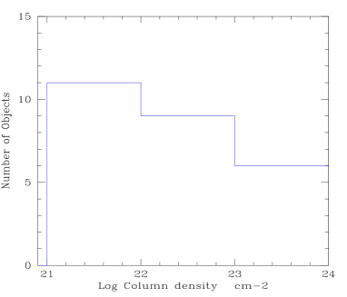
Figure 2: Distribution of the absorption column densities for the 26 sources in the sample requiring the introduction of a significant absorption component (see Table 4, Table 5; and Table 4 and 5 in Paper I).

Table 6: XMM–Newton properties of the 49 X–ray sources. Fluxes and luminosities are calculated for each source using the best–fit model listed in column 2 (see Table 5 for details).

N	Best–fit	$F_{0.5-2}^{(a)}$	$F_{2-10}^{(a)}$	$L_{2-10}^{(b)}$
	Model
42	SPL	2.08	3.79	$-$
43	WA	1.21	1.69	$-$
44	SPL	2.73	4.91	$-$
45	APL	1.78	4.38	$-$
46	SPL	1.63	2.91	$-$
47	SPL	3.18	5.01	$-$
48	APL	3.07	10.61	$-$
49	SPL	1.73	29.70	$-$
50	PL	4.39	28.1	$-$
51	APL	3.83	9.11	$-$
52	SPL	1.63	4.33	$-$
53	SPL	4.46	8.09	22.7
54	SPL	4.02	4.87	$-$
55	SPL	2.69	3.31	$-$
56	APL	0.52	3.88	$-$
57	SPL	1.71	2.11	10.8
58	PL	0.95	6.38	$-$
59	APL	36.0	76.0	1.6
60	SPL	10.64	16.55	2.2
61	SPL	7.07	4.08	7.6
62	SPL	8.97	9.82	5.1
63	PL	1.18	7.21	5.4
64	SPL	6.29	4.13	1.2
65	APL	0.12	3.98	1.7
66	SPL	3.63	4.36	27.1
67	SPL	2.00	3.40	11.5
68	SPL	5.92	13.41	3.6
69	APL	0.04	4.20	$-$
70	SPL	2.49	3.63	5.9
71	SPL	3.52	5.57	4.9
72	PL	0.23	6.76	$-$
73	SPL	1.19	1.14	$-$
74	APL	0.07	1.55	$-$
75	SPL	1.73	1.78	$-$
76	APL	0.50	1.18	$-$
77	PL	0.74	3.55	$-$
78	SPL	1.51	1.51	$-$
79	TM	1.07	1.03	$-$
80	TM	0.53	1.81	$-$
81	SPL	1.43	1.15	$-$
82	SPL	2.64	3.17	$-$
83	SPL	1.17	1.32	$-$
84	APL	0.38	2.16	$-$
85	SPL	5.12	2.49	5.8
86	SPL	3.04	4.41	$-$
87	SPL	3.27	2.76	$-$
88	APL	0.58	1.73	$-$
89	APL	1.92	5.07	$-$
90	SPL	1.96	1.65	$-$

^(a) in units of 10^-14 erg cm^-2 s^{-1  (b)} in units of 10⁴⁴ erg s^-1

The results inferred by the spectral analysis of the entire sample can be briefly summarized as follows. For about 65% (i.e. 60 out of 90) of the X–ray sources the SPL model represents an acceptable description of their spectra. 26 (out of 90) sources require the introduction of a significant absorption component (see Table 4, Table 5 and Paper I). The resulting N_H distribution is shown in Figure 2. Furthermore, 13 sources require a more complex fitting model than SPL or APL to account for a soft excess component (11 out of 13) or for the presence of warm absorber signatures (2 out of 13).

Measured values of the hard X–ray flux range from $\sim$ 1 to $\sim$ 80 $\times$ 10^-14 erg cm^-2 s^-1, with more than 50 out of 90 sources (i.e. 55%) at $F_{2-10}$ $\;\buildrel<\over{\sim}\;$ 5$\times$ 10^-14 erg cm^-2 s^-1  i.e. flux levels almost unexplored by the X–ray telescopes operating before XMM–Newton. As expected on the basis of our selection criterion, in the soft X–ray band we detect sources in a broader flux range i.e. from $F_{0.5-2}$ $\approx$ 70 down to $\approx$ 0.04 $\times$ 10^-14 erg cm^-2 s^-1. The absorption–corrected 2–10 keV luminosities span from $\approx$ 2 $\times$ 10⁴⁰ erg s^-1 to $\approx$ 5 $\times$ 10⁴⁵ erg s^-1  in agreement with the optical classification of the identified sources in the sample. All but one (i.e. NGC 4291, n. 37) sources have a $L_{2-10}$ $\;\buildrel>\over{\sim}\;$  10⁴² erg s^-1  typical of AGN: the two optically “dull” galaxies, i.e. source Nos. 3 and 41 (see Paper I), too.

Before drawing conclusions from the results of the X–ray spectral analysis, we have checked out the possible presence of systematic trends due to the source position in the detector plane which could affect photon index and/or X-ray flux measurements.

Fig. 3 shows the photon index obtained with the SPL model plotted against the hard X–ray flux: many sources have a $\Gamma$ $\sim$ 1.8–2 i.e. the typical value of unabsorbed AGNs (George et al. 2000; Nandra & Pounds 1994).

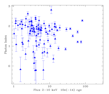
Figure 3: Photon index obtained with the SPL model as a function of the flux in the 2–10 keV band.

This matches well with the optical identifications as well as with the results obtained in the ASCA Large Sky Survey (Akiyama et al. 2000). On one hand, this plot shows that sources with flat slopes ($\Gamma\leq$ 1.3) are present at various flux levels and no trend of $\Gamma$ versus flux is evident in the data. On the other hand, despite the low number of objects at $F_{2-10}$ $\;\buildrel>\over{\sim}\;$ 10^-13 erg cm^-2 s^-1, very flat (i.e. $\Gamma$ $\;\buildrel<\over{\sim}\;$0.6) and inverted spectrum sources appear to be located in the region of the lowest fluxes as predicted by the CXB synthesis model and recently observed in Chandra deep surveys (Tozzi et al. 2001; Stern et al. 2002).

We have calculated the average SPL spectral indices in the 0.3–10 keV band for the BRIGHT and the FAINT subsamples (see Sect. 2) and obtained $\langle\Gamma\rangle$ = 1.54 $\pm$ 0.03 and $\langle\Gamma\rangle$ = 1.56 $\pm$ 0.05, respectively. These results and their comparison with the values obtained from other hard X–ray surveys will be extensively discussed in Section 6.1.

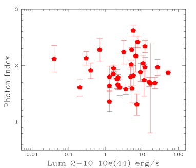
Figure 4: Spectral index, computed assuming the best fit model for all optically identified sources in the sample (except for NGC 4291), as a function of hard X–ray absorption–corrected luminosity.

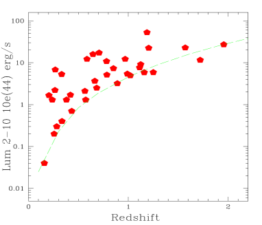
Figure 5: Intrinsic 2–10 keV X–ray luminosity plotted against redshift for the identified sources in the sample (except for NGC 4291). The dashed line indicates the “completeness” flux limit of our survey ($\sim$ 5 $\times$ 10^-14 erg cm^-2 s^-1) once all the FOVs are taken into account.

In Fig. 4 we plot the photon index as a function of the luminosity in the 2–10 keV band, as obtained applying the best fit model for each optically identified source in the sample. There is no apparent trend for spectral variations as a function of luminosity. However, a large dispersion in the slope values is present: this could either be due to intrinsic differences (George et al. 2000) or to the contribution from additional spectral components (i.e. reflection, soft–excess), unresolved here due to the limited statistics.

Fig. 5 shows the luminosity–redshift relation for the optically identified sources in the sample: as expected, the minimum and the maximum hard X–ray luminosity in each redshift bin increases with the redshift owing to a selection effect (most luminous sources are detected farthest). The present dataset is too small to disentangle any true luminosity dependence (as claimed in Barger et al. 2002) from any mere selection effects.

4.1 Multiwavelength properties of the sources

A classical approach (Maccacaro et al. 1988) extensively used in the X-ray surveys to infer some information about the nature of unidentified sources as well as to test the reliability of the optical identifications themselves is the so–called “$F_{X}$/$F_{Opt}$” diagnostic diagram. Since $R$ magnitudes are available for the majority of the sources in the sample (Table 2), we adopt this band to build such a diagnostic diagram. The relation between optical magnitude and hard X–ray flux is plotted in Fig. 6. The flux in the $R$ band is related to the $R$ magnitude by the following formula: $logF_{R}=-5.5-0.4\times R$ (Hornschemeier et al. 2001); hence, the relationship between optical flux and X–ray flux, obtained by Maccacaro et al. (1988) for the $V$ magnitude, becomes the following: $log(F_{X}/F_{R})=logF_{X}+5.5+R/2.5$.

The three dashed lines in Fig. 6 represent the X–ray to optical flux ratio of $log(F_{X}/F_{R})$ = 1, $-$1 and $-$2 (from top to bottom, respectively). They mark the regions occupied by different classes of X–ray sources as indicated in the Figure. A value comprised between $-$1 $<log(F_{X}/F_{R})<$ 1 is typical of the “standard” luminous AGNs, both of Type 1 and Type 2. As expected on the basis of the optical identifications, most of the identified sources (indicated with triangles in the Figure) are properly located in the AGN locus. Interestingly, also most of the unidentified sources (indicated with pentagons in the Figure) fall within the same region. This fact strengthens the results of our X–ray spectral analysis which indicated typical AGN–like spectra for all of them. These findings fully agree with results from hard X–ray surveys which found AGNs as the dominant population (e.g. Akiyama et al. 2000; Barger et al. 2002; Hasinger 2003).

However, there are a few sources that have values of $log(F_{X}/F_{R})$ outside the typical AGN locus. In particular, there are 4 objects (i.e. Nos. 25, 38, 63 and 65) that are notably faint in the optical with respect to their X–ray flux values. They are of particular interest because results from Chandra and XMM–Newton deep surveys (e.g. Alexander et al. 2001; Mainieri et al. 2002) suggest that this kind of sources are a mixture of “exotic” AGNs such as Type 2 QSOs, Extremely Red Objects (EROs, with $R-K$ $\;\buildrel>\over{\sim}\;$5), high redshift ($z\geq$ 3) galaxies which host a dust–enshrouded AGN and, possibly, QSOs at $z$ $\;\buildrel>\over{\sim}\;$  6.

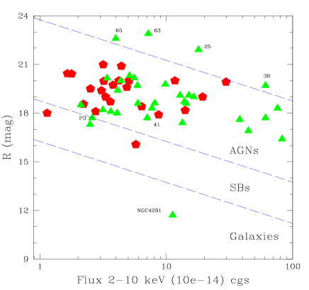
Figure 6: Plot of optical $R$ magnitude versus hard X–ray flux for those sources in the sample with available $R$ band photometry. The optically identified (unidentified) sources are indicated with triangles (pentagons). The dashed diagonal lines have been calculated following Hornschemeier et al. (2001) and represent the constant flux ratios $log(F_{X}/F_{R})=$ 1 (upper), $-$1 and $-$2 (lower). Labels show the typical $(F_{X}/F_{R})$ range observed for luminous AGN, starburst galaxies and normal galaxies in the local Universe. Peculiar sources (see text) are also indicated.

All the sources in the sample with $log(F_{X}/F_{R})>$ 1, i.e. optically–weak, are found indeed significantly X–ray absorbed as shown in Tables 4 and 5, and, interestingly, they are also all RL QSOs: two of these are also classified as narrow line QSOs of the class of EROs (i.e. Nos. 63 and 65), and the remaining two sources (i.e. Nos. 25 and 38) are optically classified as broad line QSOs. These latter show moderately flat X–ray spectra with best–fit photon indices $\Gamma\simeq$ 1.5–1.6 which are typically observed in core–dominated RL QSOs (Shastri et al. 1993; Sambruna et al. 1999; Reeves & Turner 2000). Photometric information in the $K$ band could be particularly useful to understand whether also these two QSOs could be classified as EROs as well.

At the fluxes currently sampled by our survey, the population of objects with low ($\;\buildrel<\over{\sim}\;$ –1) and very low ($<$ –2) values of $log(F_{X}/F_{R})$ are largely missed. Such kind of sources has been found to slowly emerge just below $F_{2-10}$ $\approx$ 10^-15 erg cm^-2 s^-1 and are thought to be mainly star–forming galaxies, LINERs and normal galaxies (Barger et al. 2002). These classes of sources are commonly detected in the soft X–ray band, where they are expected to be the dominat population at $F_{0.5-2}$$\;\buildrel<\over{\sim}\;$10^-17 erg cm^-2 s^-1 (Miyaji & Griffiths 2002). Three sources (Nos. 14, 73 and 85) in our sample show instead a ratio $log(F_{X}/F_{R})<$ $-$1. Among them, the first two are optically unidentified while the latter is a broad line QSO. The X–ray spectrum of this faint quasar ($F_{2-10}$ $\approx$ 2.5 $\times$ 10^-14 erg cm^-2 s^-1) is very steep ($\Gamma\sim$ 2.6, e.g. Table 3), with the source counts fairly dominated by the soft X–ray photons. This is probably the reason why we measure a value of $log(F_{X}/F_{R})$ slightly lower than unity.

As expected, the normal galaxy NGC 4291 (i.e. No. 37) is the only object with a $log(F_{X}/F_{R})<$ $-$2. Besides normal galaxies, also nearby Compton–thick AGNs usually exhibit such a low $log(F_{X}/F_{R})$ value (Comastri et al. 2003). Accordingly, it is worth noting that the peculiar sources No. 3 (the “P3” galaxy, e.g. Fiore et al. 2000) and No. 41 (that are optically identified as “normal” galaxies, see Paper I) are found to lie in the region of the diagram typical of AGNs. This finding further supports the obscured AGN nature of these two objects.

5 Hard X-ray selected QSOs

A meaningful product of our wide–angle survey consists in the opportunity of investigating at faint flux levels the spectral properties of hard X–ray selected quasars (hereafter HXSQs) and of comparing them with those derived from other studies of soft X–ray and/or optically selected QSOs.

Table 7: Properties of hard X–ray selected QSOs.

Objects	N.	$\langle\Gamma_{Best-fit}\rangle$	$\langle\Gamma_{SPL}\rangle$	$\langle L_{2-10}\rangle$a
All QSOs	30	1.87$\pm$0.04	1.66$\pm$0.03	8.97
QSOs at $z<$1	20	1.83$\pm$0.05	1.52$\pm$0.04	5.96
QSOs at $z\geq$1	10	1.96$\pm$0.05b	1.96$\pm$0.05b	14.98

^a Luminosity in units of 10⁴⁴ erg s^-1.
^b Excluding source No.85: $\langle\Gamma_{SPL}\rangle$$\equiv$$\langle\Gamma_{Best-fit}\rangle$=1.88$\pm$0.05.

In order to extract QSOs from the list of sources with optical identification, we select those showing an intrinsic 2–10 keV luminosity larger than 10⁴⁴ erg/s. In doing so, we create a sample of 30 HXSQs that is one of the largest sample of this kind available to date. Their redshifts range from $z$ = 0.205 to $z$ = 1.956 with a mean $\langle z\rangle$ $\sim$ 0.7; the vast majority of the objetcs are broad lines AGNs with the remarkable exceptions of source Nos. 63 and 65, which show an optical Type 2 classification (Table 2; Mainieri et al. 2002). The fraction of these HXSQs that turn out to be radio loud (i.e. with $\alpha_{OR}\geq$ 0.3) is 20% (i.e. 6 out of 30 sources) but, keeping in mind the incompleteness affecting the optical and radio coverage of our sample (see Table 2), this fraction should be considered only as a lower limit. Furthermore, we are able to split the sample of HXSQs in two subsamples having 10 and 20 objects each and redshift larger and lower than 1, respectively. The average properties drawn from the spectral analysis of these two samples of HXSQs (total and subsamples) are reported in Table 7, while the photon indices obtained with the SPL and with the best fit model found in each individual HXSQ are displayed in Fig. 7 and Fig. 8, respectively.

When the SPL model is applied we find a $\langle\Gamma\rangle$ = 1.66 $\pm$0.03 which rises to $\langle\Gamma\rangle$ = 1.87$\pm$0.04 using the best fit model instead. This effect can be easily explained by the presence of intrinsic absorption which suppresses the soft portion of the X–ray emission. In particular, only HXSQs at $z<$ 1, either radio–quiet (RQ) or radio–loud (RL), show this excess of absorption. Because of the limited number of HXSQs with $z>$ 1, the corresponding value of $\langle\Gamma\rangle$ appears to be biased by the very steep index of LBQS 2212–1759 (source No. 85). This source yields indeed a $\Gamma\sim$ 2.6, similar to what found by Brinkmann et al. (2003) in another bright RQ QSO: such a steep slope is reminescent of Narrow line Seyfert 1 galaxies, which usually show a strong soft excess component. However, any such soft excess component would be redshifted almost out of the EPIC energy range given the source redshift of $z$ = 1.159. In any case, a more detailed modeling of such soft excess component is not allowed due to the low photon statistics. Excluding source No. 85 from the sample, we obtain indeed an average index of $\langle\Gamma\rangle$ = 1.88$\pm$0.05, consistent with the average index found for the HXSQs at $z<$ 1. We can therefore conclude that the average X–ray spectral slope of HXSQs resulting from the present work is almost the same from $z\approx$ 0 to $z\approx$ 2 indicating no spectral evolution, i.e. no obvious variation of $\Gamma$ along the redshift (see Fig. 8).

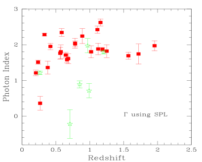
Figure 7: Plot of the full–band (0.3–10 keV) spectral index vs. redshift using SPL model for all the hard X–ray selected QSOs (HXSQs). The filled squares and the void stars are the “radio–quiet” HXSQs and the “radio–loud” HXSQs, respectively. It is worth stressing the incomplete radio coverage of our X-ray sample, so we include in “radio–quiet” HXSQs also some objects with unknown radio properties.

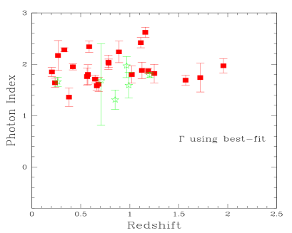
Figure 8: Same as in Figure 7, but with spectral indices derived using the best fit model for each source.

5.1 Comparison with previous works

The value of $\Gamma\approx$ 1.8–1.9 is similar to the mean slope of unobscured local Seyfert-like AGNs (i.e. $\Gamma$ = 1.86$\pm$0.05, Nandra et al. 1997; Perola et al. 2002; Malizia et al. 2003) and it matches well with previous X–ray studies of quasars carried out with different telescopes (Comastri et al. 1992; Lawson & Turner 1997). In particular, Reeves & Turner (2000) analysed a sample of 62 QSOs with ASCA, covering a redshift range from 0.06 to 4.3, and they also reported a comparable mean photon index $\langle\Gamma\rangle$ = 1.76$\pm$0.04. They also claimed a difference between the slopes of RQ QSOs ($\Gamma\sim$ 1.9) and RL QSOs ($\Gamma\sim$ 1.6), with the latter showing a flatter average photon index. This issue has been extensively discussed in Sambruna, Eracleous & Mushotzky (1999, hereafter SEM99): these authors concluded that since lobe–dominated RL QSOs have the same intrinsic photon indices of RQ QSOs, the observed harder X–ray spectra of core–dominated RL QSOs being likely due to the presence of a beamed extra–continuum component originating in the inner parts of the radio jet. For the six RL HXSQs in our sample we find a $\langle\Gamma\rangle$ = 1.66$\pm$0.17 which is slightly harder but still consistent with the typical value measured for RQ QSOs. However, it is worth noting that source Nos. 25 and 38, two bright objects with high–counting statistics, show flat photon indices ($\Gamma\sim$ 1.3 and 1.5, respectively) similar to those usually found in core–dominated RL QSOs; however in these two sources we also find that the flat spectrum is due to the presence of intrinsic absorption.

Our data also confirm that RL QSOs are characterized by absorption in excess to the Galactic value (Elvis et al. 1994): 4 out of our 6 RL objects are indeed obscured by column densities of $\approx$ 10^21-23 cm^-2. It has been suggested in other works (i.e. Cappi et al. 1997; SEM99), also on the basis of variability arguments, that such an absorber could be located in the inner nuclear regions of RL QSOs rather than associated with either the host galaxy or a surrounding cluster. Moreover, similar to our finding, SEM99 found that $\;\buildrel>\over{\sim}\;$50% of broad line RL QSOs in their sample suffered from significant intrinsic neutral absorption. These authors considered this fact at odds with simple orientation–based AGN unification models and suggested the possibility of different physical conditions of the gas around the central engine in RL QSOs, being colder in these objects than in RQ ones (George et al. 2000).

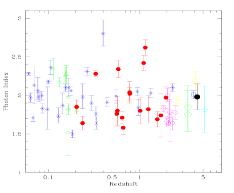
Figure 9: Photon index versus redshift for a collection of RQ QSOs observed with different X–ray telescopes. Data points are taken, respectively, from: ASCA (asterisks, Reeves & Turner 2000 and George et al. 2000), (void exagons, Vignali et al. 1999); BeppoSAX (void triangles, Mineo et al. 2000). Data from the present work are indicated with filled exagons: we have excluded the QSOs from the PKS 0312–770 field because of this field has no NVSS radio coverage. The void pentagons indicate XMMU J105144.6$+$572807 and XMMU J105125.3$+$573048 (both at $z\sim$ 3.4) which are the only RQ QSOs at $z>$ 3 from the XMM–Newton long–exposure of the Lockman Hole (Mainieri et al. 2002). The void circles represent two QSOs at $z$ = 2.64 and $z$ = 4.1 observed with XMM–Newton (Ferrero & Brinkmann 2003). The other three points at the highest redshifts correspond, respectively, to: APM 08279$+$5222 (void square; $z$ = 3.91, e.g. Hasinger et al. 2002), a joint spectrum of 9 Chandra QSOs with 4.09 $\;\buildrel<\over{\sim}\;$$z$$\;\buildrel<\over{\sim}\;$  4.51 plotted here at their average redshift (filled circle, Vignali et al. 2003) and CXO J123647.9$+$620941 (void star ; $z$ = 5.186, e.g. Vignali et al. 2002).

5.2 Spectral evolution

Concerning the evolution of the mean spectral shape, the value assessed for HXSQs by our analysis provides further support to the recent findings of Vignali et al. (2003). In fact, these authors invoke a universal X–ray emission mechanism for QSOs, i.e. indipendent from cosmic time and luminosity, on the basis of the analysis of nine high redshift ($z>$ 4) QSOs observed with Chandra. By a “stacked” spectral fitting, they found an average spectral slope of 1.98 $\pm$ 0.16 in the 2–30 keV rest–frame band (but see also Bechtold et al. 2002).

We report in Figure 9 a large compilation from literature of photon indices obtained from the spectral analysis of radio–quiet QSOs up to $z$ $\approx$ 5.2 observed with different X–ray telescopes that includes also the recent Chandra results mentioned above together with those found in the present work. No evident trend of the spectral slope appears to emerge along with the redshift from this plot, confirming that the accretion mechanism in RQ QSOs is the same at any redshift sampled to date.

6 Observational constraints for CXB synthesis models

Two main observational constraints on the predictions of synthesis models can be extracted from the present work: (1) the average slope of the sources making the CXB at intermediate flux levels and (2) the corresponding ratio of absorbed–to–unabsorbed sources. Both these parameters are essential in the definition of the average spectrum at a given flux level in order to estimate the relative contributions of individual classes of objects to the CXB.

6.1 Average slope at faint fluxes

The average photon index calculated over the 0.3–10 keV band with the SPL model is $\langle\Gamma\rangle$ = 1.59 $\pm$ 0.02. As expected, once the best fit model of each source is assumed, the resulting value of the average slope becomes steeper i.e. with a $\langle\Gamma\rangle$ = 1.80 $\pm$ 0.04. This value agrees with the typical one of unabsorbed AGNs found in previous works (e.g. Lawson & Turner 1997; Reeves & Turner 2000; Malizia et al. 2003) and it is in agreement with the classification as broad line AGNs for most of the identified sources (see Table 2).

By dividing the whole sample into the BRIGHT and the FAINT subsamples, both of which are complete at their flux limit ($F_{2-10}$ $\;\buildrel>\over{\sim}\;$ 5 $\times$ 10^-14 erg cm^-2 s^-1 and $F_{2-10}$ $\;\buildrel>\over{\sim}\;$ 2 $\times$ 10^-14 erg cm^-2 s^-1) we calculate in each case the average slope with the SPL model which turns out to be $\langle\Gamma\rangle$ = 1.54 $\pm$ 0.03 and $\langle\Gamma\rangle$ = 1.56 $\pm$ 0.05, respectively.

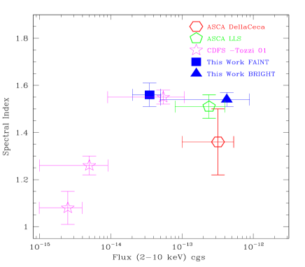
Figure 10: Average spectral index from a power model model (SPL) as a function of the hard X–ray flux. Data are taken from: Della Ceca et al. (1999; exagon), Ueda et al. (1999; pentagon), Tozzi et al. (2001; stars). The triangle (square) represents the value obtained in the present work for the BRIGHT (FAINT) subsample.

In Fig. 10 the average photon indices of the BRIGHT and FAINT samples are compared with those obtained by the most popular hard X-ray surveys carried out so far. It is worth noting that our data resulted from the spectral analysis of individual sources, whereas all other values were derived by the stacking technique. A good agreement between our values and those obtained in other works is evident from this plot.

At $F_{2-10}$ $\;\buildrel>\over{\sim}\;$1 $\times$ 10^-14 erg cm^-2 s^-1 the average slope appears still steeper than the integrated spectrum of the CXB, which has $\Gamma$ = 1.4, thus suggesting that the bulk of the flat spectrum (i.e. absorbed) sources has still to emerge at these flux levels. The measurements obtained by the Chandra Deep Field South survey (Tozzi et al. 2001; indicated as stars in Fig. 10) confirm indeed this suggestion, revealing a progressive and significative flattening of the average spectral index below $F_{2-10}$ $\;\buildrel>\over{\sim}\;$ 10 $\times$ 10^-14 erg cm^-2 s^-1, which is able to solve the “spectral paradox”.

As mentioned in Sect. 1, optical follow–up observations of X–ray deep surveys have recently pointed out that the bulk of the hard CXB is produced by a large number of narrow line active galaxies at $z\sim$ 0.7 having Seyfert–like luminosities. Consequently, we have performed a test to show how the spectral hardening occuring at $F_{2-10}$ $\sim$ 10^-15 erg cm^-2 s^-1  could be qualitatively explained by these sources. Accordingly, we have assumed a typical X-ray spectral template of a Seyfert 2 galaxy as suggested in Turner et al. (1997), i.e. a partial covering model with $\Gamma$ = 1.9, N_H = 10²³ cm^-2 and a hard X–ray (deabsorbed) luminosity of 10⁴³ erg s^-1. We have further assumed $z$ = 0.7 for the redshift value. The flux value calculated with these assumptions results to be equal to $F_{2-10}$ $\approx$ 4 $\times$ 10^-15 erg cm^-2 s^-1, i.e. well in the range where the spectral flattening has indeed been observed (Fig. 10). In addition, it is worth stressing that our simulations have shown that such a source would show a flat continuum if it were fitted with SPL model, i.e. as observed in an heavily absorbed object.

If the bulk of the hard CXB originates from a large population of Compton–thin low–redshift Seyfert 2–like galaxies, they could indeed account for the flattening of the average photon index observed by Chandra towards very faint flux levels.

6.2 Fraction of absorbed sources

Fig. 11 shows the fraction of absorbed (i.e. with an N_H $\;\buildrel>\over{\sim}\;$ 10²² cm^-2  in excess to the Galactic value) to unabsorbed sources that we find in the BRIGHT and FAINT subsamples together with those obtained by other hard X–ray surveys with different flux limits in the flux range from $F_{2-10}$ $\sim$ 10^-11 down to $F_{2-10}$ $\sim$ 10^-14 erg cm^-2 s^-1.

Interestingly, it appears from this Figure that the fraction of absorbed sources remains almost the same ($\sim$ 30%) in this wide range of hard X–ray fluxes.

It is worth noting that in order to calculate the fractions for both samples reported in this Figure we assume $\Gamma$ = 1.9 for all the sources and $z$ = 1 for the unidentified ones to overcome some biases which may affect our estimates, as mentioned in Sect. 3.1.1. The values reported in Fig. 11 can be therefore considered as conservative estimates of the fraction of absorbed sources in both samples.

6.2.1 Comparison with theoretical predictions

This finding is fairly unexpected since all synthesis models of the CXB (e.g. Gilli et al. 2001; Wilman & Fabian 1999; Comastri et al. 2001, hereafter C01) predict that as fainter fluxes are considered, more absorbed sources should be found.
In particular, in Figure 12 the theoretical predictions of the CXB synthesis model of C01 are plotted together with the fraction of absorbed sources in the 2–10 keV band found in our spectral survey.

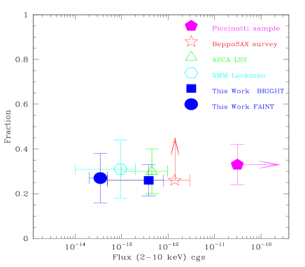
Figure 11: Fraction of absorbed sources (i.e. with N_H $\;\buildrel>\over{\sim}\;$10²² cm^-2) taken from different hard X–ray surveys. The filled square and the filled circle indicate the values found from our BRIGHT (60% optically identified, hereafter ID) and FAINT ($\sim$ 35% ID) samples, respectively. Other symbols represent the values from: Piccinotti sample (Comastri 2000, but also including 4 BL Lacs and M82 present in the original sample of Piccinotti et al. 1982; filled pentagon; 100% ID), BeppoSAX 2–10 keV survey (Giommi et al. 2000); void star), ASCA Large Area Survey (Akiyama et al. 2000; void triangle; 97% ID), and XMM–Newton survey in the Lockman Hole (Mainieri et al. 2002, void exagon; $\sim$ 90% ID). The horizontal error bars associated to the points represent the flux interval between the completeness limit and the highest flux sampled in each survey; the vertical error bars indicate instead the Poissonian errors for each fractional value.

For a better comparison we have splitted our measurement regarding the BRIGHT sample into three points. Moreover we have added the point relative to 9 $\times$ 10^-15 $\;\buildrel<\over{\sim}\;$ $F_{2-10}$ $\;\buildrel<\over{\sim}\;$  2 $\times$ 10^-14 erg cm^-2 s^-1 calculated taking into account all the sources selected in the field of LBQS 2212–1759 (this field has indeed the longest exposure time amongst the observations considered here, i.e. 80.5 ks, see Table 1) and those in the 100 ks exposure of the Lockman Hole presented in Mainieri et al. (2002).

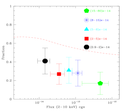
Figure 12: Fraction of absorbed sources (i.e. with N_H $\;\buildrel>\over{\sim}\;$10²² cm^-2) from our analysis vs. 2–10 keV flux compared to theoretical prediction of Comastri et al. (2001). For the calculation of our points we assumed a conservative spectral slope of $\Gamma$=1.9 for all sources and $z$ = 1 whenever the X–ray source was not optically identified. The value for the point at faintest flux has been calculated using sources selected in the deepest exposure of ours (i.e. the LBQS 2212$-$1759 filed, 80.5 ks) together with sources in the 100 ks exposure of the Lockman Hole analysed by Mainieri et al. (2002).

This figure shows that the fraction of absorbed sources predicted by the theory is a factor of $\sim$ 2 larger (with a $\approx$ 4.5$\sigma$ significance) than our observational data at comparable fluxes. We thus confirm and extend even to fainter fluxes the data–to–model mismatch found in Paper I. Our data suggest that unabsorbed (i.e.with N_H $\;\buildrel<\over{\sim}\;$ 10²² cm^-2) objects still largely dominate the source counts at $F_{2-10}$ $\;\buildrel>\over{\sim}\;$10^-14 erg cm^-2 s^-1, at odds with the theoretical expectations of about 50–60% of absorbed sources.

Despite this mismatch, the overall trend predicted by the model follows the observational data as if only the normalization was wrong.

Although very preliminary, also the results of the individual spectral analysis of the brightest X–ray sources in the HDFN (Bauer et al. 2003) seem to suggest a N_H distribution peaked towards low column density values with only few sources ($<$ 9%) obscured by N_H $\;\buildrel>\over{\sim}\;$ 10²³ cm^-2 whereas the synthesis models predict a value of $\sim$ 20%. Other works based on hardness ratios analyses further confirm such a scarsity of obscured objects above $F_{2-10}$ $\sim$ 10^-14 erg cm^-2 s^-1  (e.g. Baldi et al. 2002; Akiyama, Ueda & Otha 2002): in particular the latter authors reported a fraction of absorbed source with N_H $\;\buildrel>\over{\sim}\;$ 10²² cm^-2 and $L_{2-10}$ $>$ 10⁴⁴ erg s^-1 of $\sim$ 15%, i.e. a factor of 3 lower than expected.

Furthermore, the average photon index values at $F_{2-10}$ $\;\buildrel>\over{\sim}\;$ 10^-14 erg s^-1 reported in the present as well as in other works (Sect. 6.1) result to be steeper than the slope of the integrated CXB spectrum: this result is indicative of the fact that absorbed objects are not yet present in large quantities at these fluxes, as suggested instead by theoretical models.

Possible explanations for this observational mismatch will be extensively discussed in Sect. 7.

6.3 Comparison with the results from the 1Ms HDFN survey

Since this data/model mismatch on the fraction of absorbed sources has been claimed in Paper I and in the present paper for the first time, it requires further investigations before validation. We have thus used the data from the Chandra 1Ms Hubble Deep Field North survey published in Brandt et al. (2001) to estimate the fraction of absorbed versus unabsorbed objects at our flux levels and lower.

To this aim, from the entire X–ray source catalog only the sources detected in the 2–8 keV band (265) have been selected. Their fluxes span a very large range i.e. 1.4 $\times$ 10^-16 $\;\buildrel<\over{\sim}\;$ $F_{2-8}$ $\;\buildrel<\over{\sim}\;$  1.2 $\times$ 10^-13 erg cm^-2 s^-1. Of these 265 sources, Barger et al. (2002) presented the optical identification for 118 (i.e. $\sim$ 45%).

Since Brandt et al. (2001) used the source fluxes corrected for vignetting, we calculate source–by–source the “flux ratio” $FR$ rather than the commonly–used “hardness ratio”. This ratio is defined as follows:

$FR$ = ($F_{2-8}$ – $F_{0.5-2}$)/($F_{2-8}$ $+$ $F_{0.5-2}$)

Similarly to the “hardness ratio”, this quantity is indicative of the “flatness” of an X–ray spectrum. Accordingly, sources with $FR$ = 1 represent those without a positive detection in the soft X–ray band but seen in the hard X–ray band. We then compare the $FR$ value of every source with that (hereafter indicated with $FR_{z}$) obtained for an object with $\Gamma$ = 1.7, N_H = 10²² cm^-2 placed at the redshift of that source (or $z$ = 1 for an optically unidentified one). Accordingly, a source that shows $FR>$ $FR_{z}$ is X–ray obscured with an N_H $>$ 10²² cm^-2.

Following this procedure, it is possible to estimate the fraction of absorbed sources in the Chandra HDFN 1Ms exposure at different hard X–ray flux levels. These results are displayed in Figure 13 together with those derived from our analysis.

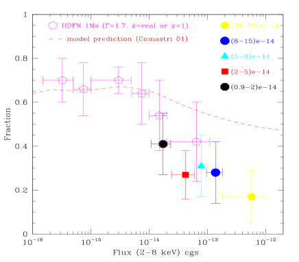
Figure 13: Ratios of absorbed (N_H $\;\buildrel>\over{\sim}\;$ 10²² cm^-2) to unabsorbed hard X–ray selected sources in our sample (filled symbols) and in the HDFN 1Ms exposures (void pentagons) as a function of the 2–8 keV flux compared to model predictions (dashed line; Comastri et al. 2001). Points from our analysis are the same as those plotted in Fig. 12, but at flux values smaller than a factor of 1.2 ($F_{2-10}$/$F_{2-8}\sim$ 1.2 with $\Gamma$ = 1.7) in order to provide a better comparison with HDFN data. The values from the HDFN has been derived taking into account X–ray and optical data from Brandt et al. (2001) and Barger et al. (2002), respectively. We obtained the fractions of absorbed sources in each flux bin by means the “flux–ratio”, i.e.: $FR$ =($F_{2-8}-$$F_{0.5-2}$)$/$($F_{2-8}+$$F_{0.5-2}$), analysis. We consider “absorbed” a source with an $FR$ value larger than that calculated assuming $\Gamma$ = 1.7, N_H = 10²² cm^-2 and the redshift proper of the source or $z$ = 1 if the X–ray source is not optically identified (see text for further details).

It appears from Figure 13 that at hard X–ray fluxes from $\approx$ 10^-14 erg cm^-2 s^-1 down to $\approx$ 10^-16 erg cm^-2 s^-1  the fraction calculated in the HDFN data matches very well with the model predictions. On the other hand, the two points at $F_{2-8}>$ 10^-14 erg cm^-2 s^-1  are consistent both with the theoretical values and our estimates. However, it is worth noting the large errors which affect the Chandra measurements: in fact, due to their lower number densities per deg², the number of objects detected at the brightest fluxes by this 1 Ms exposure is relatively small, with only 34 X–ray sources having $F_{2-8}>$ 10^-14 erg cm^-2 s^-1. Furthermore, some flat spectra could be due to warm absorber features rather than cold absorption material and unfortunately hardness ratio analysis does not allow to discriminate between the two.

The analysis of this ultra–deep Chandra observation therefore confirms only partially our finding. Unfortunately, it does not provide an efficient tool to disentangle the mismatch reported in Section 6.2.

This result is however very useful as it provides the most accurate estimate never published elsewhere for the fraction of absorbed sources at flux levels much fainter than those sampled in our survey ($\;\buildrel<\over{\sim}\;$10^-15 erg cm^-2 s^-1).

7 How to explain this data/model mismatch?

7.1 Observational biases

There are three main observational biases which may affect our estimate of the fraction of obscured sources, i.e.:

1. Poor statistics from the faintest sources. This fact may have lead in some cases to a possible underestimate of the real N_H value because of the possible presence of an unresolved soft–excess or reflection component.

   However, we consider that this bias is in large part taken into account by fixing the photon index to $\Gamma$ = 1.9 before re–estimating the amount of cold absorption column density (see Sect. 3.1.1). Moreover, as reported in Sect. 4.2.2 of Paper I, we performed simulations in order to rule out the possibility that we miss some obscured sources at fluxes above the completeness limit of our survey.

2. Incompleteness of the optical identifications. The column density measured in the optically unindentified sources would be certainly underestimated if they were placed at $z$ = 0 (see Sect. 3.1.1). Nevertheless, we estimate that we overcome this bias by assuming $z$ = 1 for such sources, i.e. by placing them just above the peak of the newly observed redshift distribution (e.g. Hasinger 2003; Barger et al. 2002) in order to provide a more conservative estimate of their N_H values.

3. Selection effect due to the PN effective area. The predictions shown in Fig. 12 and Fig. 13 have been calculated assuming a flat–response detector (C01). This is not the case of XMM–Newton, whose effective area, although the best to date, is affected by a degradation by about a factor of two between 4 and 9 keV. Hence, a convolution of the models with the response of EPIC would be very important in order to allow a proper comparison between the observational data and the theoretical expectations.

   Interestingly, if we rescrict the analysis to the 5–10 keV energy band and compare the fraction of absorbed objects resulting from the complete subsample of 22 sources with $F_{5-10}$ $\;\buildrel>\over{\sim}\;$ 5 $\times$ 10^-14 erg cm^-2 s^-1 with the model prediction in this band, we still notice that our value is $\sim$ 30%, i.e. a factor of 2 lower than expected by C01 ($\sim$ 60%).

7.2 Revision of some model assumptions

We address here the possibility that one (or more) of the assumptions usually included in synthesis models of the CXB need to be revised. The results presented here and the mismatch emerging in the optical follow–up of the deep X-ray surveys (Hasinger 2003) between the predicted and the observed redshift distribution of X–ray sources indeed suggest that some inputs of the CXB theoretical models should be updated.

The most critical assumptions usually made in theoretical works are three: the spectral template adopted for the X–ray sources, the distribution of absorption column densities and the slope, form and evolution of the X–ray luminosity function (XLF), which is almost unknown for Type 2 objects.

1. The X–ray spectral properties. Although the overall X–ray spectral shape of AGN is thought to be known (Mushotzky et al. 1993, Nandra & Pounds 1994), some details are still uncertain.

   For example, the average value of the high–energy cutoff (due to thermal Comptonization) is poorly constrained. Most theoretical models assume $E_{cutoff}$ = 320 keV (C01, Gilli et al. 1999), but this is certainly a rough approximation. On the basis of BeppoSAX observations Matt (2000), Perola et al. (2002) and, recently, Malizia et al. (2003) clearly showed that the average cutoff value is more around 120–180 keV.

   It is worth noting that the high–energy cutoff is one of the key parameters in reproducing the peculiar “bump–like” shape of the CXB. The ubiquitous presence of an upward curvature (the so–called soft–excess) rising steeply below 2 keV in the spectrum of unabsorbed AGNs is also uncertain (Matt 2000), especially in the case of luminous objects (Reeves & Turner 2000, George et al. 2000).

   All the above spectral properties are still to be well constrained for the brightest sources in the local Universe and, mostly, there is a evident lack of information about their possible evolution along $z$ and/or luminosity.

2. The N_H distribution. Gilli et al. (1999) and Gilli et al. (2001) assumed in their models a “fixed” distribution of the absorbing column densities for Type 2 objects. They used the distribution found by Risaliti et al. (1999) for a sample of nearby optically–selected Seyfert 2 galaxies. There are three main causes of uncertainty in their assumption: ($i$) the observed distribution is based on a limited luminosity range; ($ii$) it takes into account only “optical” Type 2 AGNs i.e. objects with narrow emission lines in their optical spectra (but, as extensively discussed in Paper I, a mismatch between optical and X–ray classification of AGN has been widely observed) and, most important, ($iii$) such distribution has been derived from sources in the local Universe (which are clearly not responsible for the bulk of the CXB). Consequently, the assumptions made in their model regarding the extension of the N_H distribution to higher redshifts could be erroneous, thus introducing an error in the final output of their estimation.

3. The XLF of Type 2 AGNs. Recent results from optical follow–ups of Chandra and XMM–Newton  deep surveys yield a source redshift distribution that, if confirmed, would require a substantial revision of the commonly assumed XLFs (Hasinger 2003; Cowie et al. 2003).

   The main uncertainty in all synthesis models of the CXB is indeed the XLF of obscured sources and its cosmological evolution, both of which are completely unknown. So far theoretical models have assumed the same XLF for Type 1 and Type 2 AGNs. However, on the basis of the above results (i.e. the bulk of the CXB originates from narrow line AGNs at $z$$\;\buildrel<\over{\sim}\;$ 1), it has been suggested that the evolution properties of Type 2 sources is likely to be different from that of Type 1s.

   Moreover, the commonly–used XLFs of Type 1 AGNs have been mainly derived from soft X–ray surveys and, in addition, their evolution with $z$ is still debated (Comastri 2000 for a complete review).

   An attempt to adapt the theory to the new observational evidences, has been recently done by Franceschini, Braito & Fadda (2002, hereafter FBF02). These authors have proposed a model for the CXB where the obscured AGNs closely follow the evolution of strongly evolving infrared starburst galaxies (as recently found by ISO surveys), which evolve steeply up to $z\sim$ 0.8 similarly to the X-ray sources detected in the deep surveys (Cowie et al. 2003). This approach is based on the fact that $\sim$ 65% of the sources (mostly AGNs) detected in the Lockman Hole survey in the 5–10 keV band have an IR counterpart at 15 $\mu$m. FBF02 therefore suggested two different evolutionary patterns for Type 1 and Type 2 AGNs: the former evolve as given by optical and soft X–ray surveys, whereas the latter evolve faster, as found in mid–IR surveys.

   However, this scenario seems to be more complicated than described by FBF02 (and subsequently refined by Gandhi & Fabian 2003): in fact, Gilli (2003) has shown that such a “starburst–like” evolution for Type 2 objects largely overestimates the ratio of obscured–to–unobscured objects at $z$ $\;\buildrel<\over{\sim}\;$ 1.

4. Space density evolution of different AGN types. Another hypothesis is that classes of AGN with different luminosity may evolve differently, contrary to what generally assumed in theoretical models, where the evolution is modeled only taking into account unabsorbed QSOs.

   In particular, Cowie et al. (2003) and Barger et al. (2003) have recently suggested on the basis of Chandra data that the space density evolution for Seyfert–like objects could be nearly constant (or, at most, slightly declining above $z>$ 0.7) up to $z$ $\sim$ 2.5, while that of high–luminosity QSO–like AGNs shall increase rapidly from $z\sim$ 0 up to $z\sim$ 3 in agreement with the evolution of optically–selected samples.

The need for more accurate XLFs both for obscured and unobscured sources clearly emerges from this discussion. This information is indeed a crucial input for all models aimed at achieving a correct and complete interpretation of the CXB phenomenon.

To date, it appears difficult to predict how all this new information obtained by Chandra and XMM–Newton will affect synthesis models of the CXB. It is beyond the goal of this paper to estimate what type of changes these new observational constraints (including our new measurement of the fraction of absorbed versus unabsorbed objects) will put on these models, but it will be clearly an important development for future theoretical works.

8 Conclusions

This work provides the first step in the detailed study of the X–ray spectral properties of hard X–ray selected sources detected at faint fluxes (i.e. $F_{2-10}$ $\;\buildrel<\over{\sim}\;$ 10^-13 erg cm^-2 s^-1) near the knee of the Log$N$–Log$S$ distribution. These are the sources that most contribute to the CXB.

Previously published works on this topic were based mainly on hardness ratio and/or stacked spectral analyses. Complementary to ultradeep pencil–beam surveys, our shallower survey addresses for the first time the analysis of each individual spectrum.

Results have been reported for a sample of 90 hard X–ray selected sources detected serendipitously in twelve EPIC fields. This is the largest ever made sample of this type. A detailed spectral analysis has been performed in order to measure source-by-source the 0.3–10 keV continuum shape, the amount of cold (and, possibly, ionized) absorbing matter and the strength of other spectral features such as soft excess and warm absorber components.

The most important results can be briefly outlined as follows:

1. Fluxes in the 2–10 (0.5–2) keV band span from 1 (0.04) to 80 (70) $\times$ 10^-14 erg cm^-2 s^-1. About 40% of the X–ray sources are optically classified from the literature. Most of them are broad line AGNs with redshift in the range 0.1 $\;\buildrel<\over{\sim}\;$ $z$ $\;\buildrel<\over{\sim}\;$ 2. The high luminosities found (10⁴² $\leq L_{2-10}\leq$ 10⁴⁵ erg s^-1) match well with these identifications except for two “optically dull” galaxies (see also Paper I).

2. Using a simple power law model with Galactic absorption we obtain $\langle\Gamma\rangle$ = 1.59$\pm$0.02. Considering only sources in the BRIGHT and FAINT subsamples we find $\langle\Gamma\rangle$ = 1.53$\pm$0.03 and $\langle\Gamma\rangle$ = 1.56$\pm$0.05, respectively. Both these values are in fairly good agreement with stacked spectral analysis obtained from ASCA and Chandra hard X–ray surveys.

3. 65% of the sources are well fitted with the SPL model; their average spectrum provides a photon index $\Gamma\sim$ 1.7$\div$2.0, i.e. typical of unabsorbed AGNs.

4. 30% of the sources require a column density larger than the Galactic value with N_H ranging from $\approx$ 10²¹ to $\approx$ 10²³ cm^-2 (Sect. 4). In particular, two narrow line AGNs turn out to be Type 2 QSOs since they are characterized by high luminosities ($L_{2-10}>$ 10⁴⁴ erg s^-1) and high column densities (N_H $>$ 10²² cm^-2).

5. The mean slope of hard X–ray selected QSOs in our sample remains nearly constant ($\langle\Gamma\rangle\approx$ 1.8–1.9) between $z\sim$ 0 and $\sim$ 2 (Sect. 5). By combining this result with other recent works on high–$z$ QSOs, we strengthen the suggestion that QSOs do not exhibit any spectral evolution and, hence, the type of accretion in these objects should be similar up to $z\approx$ 5.

6. While from the analysis of the sources detected in the 1Ms HDFN survey at faint fluxes ($F_{2-10}$ $<$ 10^-14 erg cm^-2 s^-1) the observed fraction of absorbed sources (N_H $\;\buildrel>\over{\sim}\;$ 10²² cm^-2) is consistent with the theoretical predictions, at the brighter fluxes ($F_{2-10}$ $\;\buildrel>\over{\sim}\;$ 10^-14 erg cm^-2 s^-1) considered in our survey it appears to be a factor $\sim$ 2 lower (with a $\approx$ 4.5$\sigma$ significance) than predicted by synthesis models of the CXB. This confirms and extends our previous results obtained in Paper I.

- (1) Akiyama, M., Ohta, K., Yamada, T., et al. 2000, ApJ 532, 700
- (2) Akiyama, M., Ueda, Y., & Ohta, K., 2002, Proc. of IAU Colloquium 184 ”AGN Surveys” (18-22 June 2001, Armenia)
- (3) Alexander, D.M., Brandt, W.N., Hornschemeier, A.E., et al., 2001, AJ 122, 2156
- (4) Baldi, A., Molendi, S., Comastri, A., et al., 2002, Proc. of “New Visions of the Universe in the XMM-Newton and Chandra era”, F. Jansen et al. (ed), (astro-ph/0201525)
- (5) Barger, A.J., Cowie, L.L., Brandt, W. N., et al., 2002, ApJ 124, 1839
- (6) Barger, A.J., Cowie, L.L., Capak, P., et al., 2003, ApJ 584, L61
- (7) Bauer, F.E., Vignali, C., Alexander, D.M., et al., 2003, AN, in press
- (8) Bechtold, J., Siemiginowska, A., Shields, J., et al., 2002, ApJ in press, (astro-ph/0204462)
- (9) Brandt, W. N., Alexander, D.M., Hornschemeier, A.E., et al., 2001, AJ 122, 2810
- (10) Brinkmann, W., Grupe, D., Branduardi-Raymont, G., Ferrero, E., 2003, A&A 398, 81
- (11) Cappi, M., Matsuoka, M., Comastri, A., et al., 1997, ApJ 478, 492
- (12) Comastri, A., Setti, G., Zamorani, G., et al., 1992, ApJ 384, 62
- (13) Comastri, A., Setti, G., Zamorani, G., & Hasinger, G., 1995, A&A 296,1
- (14) Comastri, A., 2000, Proc. of “X-ray Astronomy ’99: Stellar Endpoints, AGNs and the Diffuse X-ray Background”, (astro-ph/0003437)
- (15) Comastri, A., Fiore, F., Vignali, C., et al. 2001, MNRAS 327, 871
- (16) Comastri, A., Brusa, M., Mignoli, M., et al. 2003, AN 324, 28
- (17) Cowie, L.L., Barger, A.J., Bautz, M.W., et al. 2003, ApJ 584, 57
- (18) De Zotti, G., Boldt, E. A., Marshall, F. E., et al., 1982, ApJ 253, 47
- (19) Elvis, M., Fiore, F., Wilkes, B., et al., 1994, ApJ 422, 60
- (20) Ferrero, E., & Brinkmann, W., 2003, A&A, in press
- (21) Fiore, F., Comastri, A., La Franca, F., et al., 2001, Proc. of ESO Conference “Deep Fields”, (astro-ph/0102041)
- (22) Franceschini, A.,Hasinger, G., Miyaji, T., Malquori, D., 1999, MNRAS 310, L5
- (23) Franceschini, A., Braito, V., & Fadda, D., 2002, MNRAS 335, L51
- (24) Gandhi, P., & Fabian, A.C., 2003, MNRAS 339, 1095
- (25) Gehrels,1986, ApJ 303, 336
- (26) George, I.M., Turner, T.J., Yaqoob, T., et al., 2000, ApJ 531, 52
- (27) Gilli, R., Risaliti, G., Salvati, M., 1999, A&A 347, 424
- (28) Gilli, R., Salvati, M., & Hasinger, G., 2001, A&A 366, 407
- (29) Gilli, R., 2003, AN 324, 165
- (30) Giommi, P., Perri, M., & Fiore, F., 2000, A&A 362, 799
- (31) Hasinger, G., Altieri, B., Arnaud, M., et al., 2001, A&A 365 , L45
- (32) Hasinger, G., Schartel, N., & Komossa, S., 2002, ApJ 573, L77
- (33) Hasinger, G., 2003, Proc. of the 13th Annual Astrophysics Conference in Maryland (”The Emergence of Cosmic Structure”), Eds. Stephen M., Holt, S., & Reynolds, C.
- (34) Hornschemeier, A.E., Brandt, W.N., Garmire, G.P., et al., 2001, ApJ 554, 742
- (35) Jansen, F., Lumb, D. H., Altieri, B., et al., 2001, A&A 365, L1
- (36) Kinkhabwala, A., Sako, M., Behar, E., et al., 2002, Proc. of the symposium “New Visions of the X-ray Universe in the XMM–Newton and Chandra Era”, 26-30 November 2001, ESTEC, The Netherlands
- (37) Lawson, A.J., Turner, M.J.L., 1997, MNRAS 288, 920
- (38) Maccacaro, T., Gioia, I. M., Wolter, A., et al. 1988, ApJ 326, 680
- (39) Mainieri , V., Bergeron, J., Hasinger, G., et al. 2002, A&A 393, 425
- (40) Malizia, A., Bassani, L., Stephen, J.B., et al., 2003, ApJ in press, (astro-ph/0304133)
- (41) Matt, G., 2000, Proc. of “X-ray Astronomy ’99: Stellar Endpoints, AGNs and the Diffuse X-ray Background”, (astro-ph/0007105)
- (42) Mineo, T., Fiore, F., Laor, A., et al. 2000, A&A 359, 471
- (43) Miyaji, T., & Griffiths, R.E., 2002, ApJ 564, L5
- (44) Moretti, A., Campana, S., Lazzati, D., & Tagliaferri, G., 2003, ApJ in press
- (45) Mukai, K., 2000, PIMMS Version 3.0 Users Guide (Greenbelt: NASA/GSFC)
- (46) Mushotzky, R.F., Done, C., & Pounds, K.A., 1993, ARA&A 31, 717
- (47) Mushotzky, R.F., Cowie, L.L., Barger, A.J., & Arnaud, K.A., 2000, Nature 404, 459
- (48) Nandra, K., & Pounds, K.A., 1994, MNRAS 268, 405
- (49) Nandra, K., George, I.M., Mushotzky, R.F., et al., 1997,
- (50) Perola, C., Matt, G., Cappi, M., et al.,2002, A&A 389, 802
- (51) Piconcelli, E., Cappi, M., Bassani, L., et al., 2002, A&A, 394, 835 (Paper I)
- (52) Piconcelli, E., 2003, Ph.D. Thesis, Università di Bologna
- (53) Reeves, J.N., Turner, M.J.L., 2000, MNRAS 316, 234
- (54) Reynolds, C.S., 1997, MNRAS 286, 513
- (55) Rosati, P., Tozzi, P., Giacconi, R., et al., 2002, ApJ 566, 667
- (56) Sambruna, R.M., Eracleous, M., & Mushotzky, R.F., 1999, ApJ 526, 60
- (57) Shastri, P., Wilkes, B.J., Elvis, M., McDowell, J., 1993, ApJ.410, 29
- (58) Silk, J., & Rees, M.J., 1998, A&A 331, L1
- (59) Stern, D., Tozzi, P., Stanford, S.A., et al., 2002, AJ 123, 2223
- (60) Struder, L., Briel, U., Dennerl, K., et al., 2001, A&A 365, L18
- (61) Tozzi, P., Rosati, P., Nonino, M., et al. 2001, ApJ 562, 42
- (62) Turner,T.J., George, I.M., Nandra, K., & Mushotzky, R.F., 1997, ApJ 488, 164
- (63) Turner, M.J.L.T., Abbey, A., Arnaud, M., et al., 2001, A&A 365, L27
- (64) Vignali, C., Comastri, A., Cappi, M. et al., 1999, ApJ 516, 582
- (65) Vignali, C., Bauer, F., Alexander, D.M., et al., 2002, ApJ 580, L105
- (66) Vignali, C., Brandt, W.N., Schneider, D.P., et al., 2003, AJ 125, 418
- (67) Wilman, R.J., & Fabian, A. C., 1999, MNRAS 309, 862