Distribution of Faraday Rotation Measure
in Jets from Active Galactic Nuclei
I. Prediction from our Sweeping Magnetic Twist Model

Abstract

Using the numerical data of MHD simulation for AGN jets based on our “sweeping magnetic twist model”, we calculated the Faraday rotation measure (FRM) and the Stokes parameters to compare with observations. We propose that the FRM distribution can be used to discuss the 3-dimensional structure of magnetic field around jets, together with the projected magnetic field derived from the Stokes parameters. In the present paper, we supposed the basic straight part of AGN jet, and used the data of axisymmetric simulation. The FRM distribution we derived has a general tendency to have gradient across the jet axis, which is due to the toroidal component of the helical magnetic field generated by the rotation of the accretion disk. This kind of gradient in the FRM distribution is actually observed in some AGN jets (e.g. Asada et al. 2002), which suggests helical magnetic field around the jets and thus supports our MHD model. Following this success, we are now extending our numerical observation to the wiggled part of the jets using the data of 3-dimensional simulation based on our model in the following paper.

1 Introduction

To explain the formation of active galactic nucleus (AGN) jets and other astrophysical jets, various models have been proposed. Among them, magnetohydorodynamic (MHD) model is one of the most promising models, since it can explain both the acceleration and the collimation of the jets. Lovelace (1976) and Blandford (1976) first proposed the magnetically driven jet from accretion disks, and Blandford & Payne (1982) discussed magneto-centrifugally driven outflow from a Keplerian disk in steady, axisymmetric and self-similar situation. Uchida & Shibata (1985) performed a time-dependent, two-dimensional axisymmetric simulation in the case of star-forming outflows. They pointed out that large amplitude torsional Alfvén waves (TAW’s) generated by the interaction between the accretion disk and a large scale magnetic field play an important role (detail is described in section 2). In this paper, we refer this model as ”sweeping magnetic twist model”. Uchida & Shibata (1986) extended the treatment to the case of AGN jets. After this work, many authors have performed time-dependent, two-dimensional axisymmetric simulations (e.g. Stone & Norman 1994, Ustyugova et al. 1995, Matsumoto et al. 1996, Ouyed & Pudritz 1997, Kudoh, Matsumoto, & Shibata 1998). Acceleration mechanisms in MHD model were studied in detail by 1.5-dimensional MHD equations (Kudoh & Shibata 1997a, 1997b).

Using the numerical data of MHD model, observational quantities such as the Faraday rotation measure (FRM) or the Stokes parameters have been derived to compare with observations of AGN jets: Laing (1981) computed the total intensity, the linear polarization, and the projected magnetic field distributions, assuming some simple magnetic field configurations and high energy particle distributions in the cylindrical jet. Clarke, Norman, & Burns (1989) performed two dimensional MHD simulations in which a supersonic jet with a dynamically passive helical magnetic field was computed, and derived distributions of the total intensity, the projected electric field, and the linear polarization. Hardee & Rosen (1999) calculated the total intensity and the projected magnetic field distributions, using 3-dimensional MHD simulations of strongly magnetized conical jets. Hardee & Rosen (2002) calculated the FRM distribution and discussed that the radio source 3C465 in Abell cluster A2634 (Eilek & Owen 2002) suggests helical twisting of the flow.

The FRM is given by the integral of $n_{e}B_{\parallel}$ along the line-of-sight between the emitter and the observer (where $B_{\parallel}$ is the line-of-sight component of the magnetic field, and $n_{e}$ is the electron density there). It is, in principle, not possible to specify which part on the line-of-sight the contribution comes from. However, in recent high-resolution radio observations (e.g. Eilek & Owen 2002, Asada et al. 2002), the FRM distribution seems to have good correlation with the configuration of the jet; this suggests that the FRM variation is due to the magnetized thermal plasma surrounding the emitting part of the jet. In fact, sharp FRM gradients seen in 3C273 can not be produced by a foreground Faraday screen (Taylor 1998, Asada et al. 2002). If this is the case, we can get a new information, that is, the line-of-sight component of the magnetic field, and thus can predict the 3-dimensional configuration of the magnetic field around the jet, together with the projected magnetic field.

In this paper, we calculate the FRM, projected magnetic field, and total intensity from the numerical data of MHD simulation based on our “sweeping magnetic twist model”, and discuss these model counterparts comparing with some observations. Here we consider the straight part of the jet, and thus use the data of axisymmetric simulation. In section 2, we review the physics of our ”sweeping magnetic twist model”. We introduce the method to calculate model counterparts of observational quantities in section 3, and show the results in section 4. Comparisons of model counterparts with some observations are discussed in section 5.

2 Brief Review of Our “Sweeping Magnetic Twist Model”

In this section, we briefly review the results of 2.5-dimensional MHD simulations based on our “sweeping magnetic twist model” to discuss the magnetic field around the straight part of jets. In the following paper, we will extend our treatment to the wiggled part of jets, which we have given an interpretation using a 3-dimensional MHD simulation based on our model (Nakamura, Uchida, & Hirose 2001).

In the original MHD model (Uchida & Shibata 1985) for bipolar outflows in star-forming regions, they considered a gravitational contraction of magnetized gas to form a star (plus an accretion disk). They attributed the large scale magnetic field to the weak field in the Galactic arms. It is strengthened in the process of gravitational contraction of the interstellar gas to the star-forming core, and plays a critical role. The toroidal field is continuously produced from the poloidal field by the rotation of the accretion disk. This causes magnetic braking to the disk material, and the material which loses angular momentum falls gradually toward the central gravitator, and releases the gravitational energy. A part of the released gravitational energy is supplied to the jets along the magnetic field. The produced toroidal magnetic field propagates into two directions along the bunched large scale magnetic field as large amplitude TAW’s. These TAW’s serve to collimate the large scale poloidal field into the shape of a slender jet by dynamically pinching it in the propagation (“sweeping pinch effect”). This process, verified in the simulation, was proposed by Uchida & Shibata (1985) as a generic magnetic effect operating in the formation of astrophysical jets utilizing gravitational energy.

The mechanism was applied to the case of AGN jets (Uchida & Shibata 1986) by supposing that a large scale intergalactic magnetic field plays the role in the case of the formation of a protogalaxy and a giant black hole at its core. They argued that the same process as in the star formation case is applicable to the AGN jet cases with more or less similar set up (having accretion disk around the central gravitator etc.), due to the similarity of the basic equation system. One of the possible differences between AGN jets and the star formation jets may be the relativistic effects. The effect of general relativity will be appreciable very close to the central giant black hole comparable to the Schwarzschild radius (Koide, Shibata, & Kudoh 1998). There are regions in which the special relativity should be taken into account when the Alfvén velocity estimated in the classical definition is close to or exceed the velocity of light. Here in this paper, we concentrate ourselves on the essential physical process in the production and collimation of the jet in the non-relativistic range.

The problem was treated with the non-linear system of MHD equations in a time dependent way for the first time when they proposed this model in 1985. The numerical approach was so-called axial 2.5-dimensional approximation, where the quantities are axisymmetric, but the azimuthal components of vectors are included to allow them play very essential roles such as centrifugal effect or pinch effect. Thus the authors were able to deal with the physical driving and collimating mechanism they proposed to be in operation for astrophysical jets.

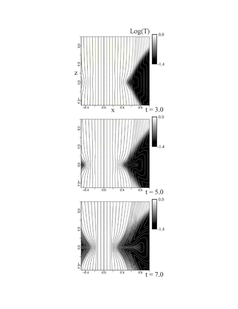
Figure 1: Time development in the $r-z$ plane in our 2.5-dimensional MHD simulation near the central core. The distribution of logarithmic temperature is shown in gray-scale. Curves represent the poloidal magnetic field.

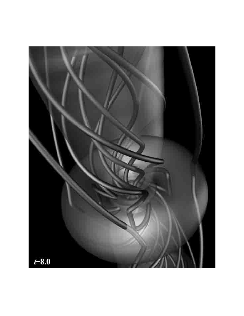
Figure 2: 3-dimensional presentation of the magnetic field with the accretion torus and jets (Meier, Koide, & Uchida 2001, Front page of Science).

Figure 1 shows the time development in the 2.5-dimensional MHD simulation based on our model. The rotating gas pulls the magnetic field gradually inward, which twists up the magnetic field because the rotational velocity is faster as close to the center (Figure 2). This continuously supplies large amplitude TAW’s (Poynting flux) along the external magnetic field, which pinch the poloidal magnetic field into the shape of a slender jet as discussed in the above. The gas in the surface of the torus is swirled out into two directions along the axis, both by the magnetic pressure gradient and the centrifugal effect. Thus the propagation of the torsional Alfvén wave accelerates the gas in the surface of the disk into the spinning jets.

It is noted that the accretion toward the central gravitator takes place in the form of avalanches from upper and lower surfaces of the geometrically thick torus (Matsumoto et al. 1996), because the transfer of angular momentum to the external magnetic field is most efficient there. The magnetic fields of opposite polarity, brought with the accretion flows avalanching on the surfaces of the disk, make reconnection at the innermost edge of the disk in the equatorial plane (Figure 1). This process will contribute to the supply of the “seed high energy particles” into the jet. Such particles will be re-accelerated through the Fermi-I acceleration process when two TAW fronts trapping the particles in between them approach to each other, for example, as the foregoing one is decelerated due to an encounter with high density gas blob remaining in the collapse (Uchida et al. 1999).

3 Method of Calculation of Model Counterparts

Using the numerical data of the 2.5-dimensional simulation explained in the previous section, we computed the distributions of the FRM, the projected magnetic field, and the total intensity with some viewing angles.

We computed the FRM distribution by integrating $n_{e}B_{\parallel}$ along the line-of-sight (Hardee & Rosen 2002). To calculate the Stokes parameters, we assume the following: (1)radiation process is synchrotron radiation, (2)synchrotron self absorption is negligible, (3)the spectral index, $\alpha$, is equal to unity, and (4)the projected magnetic field is perpendicular to the projected electric field. The emissivity of the synchrotron radiation is given by $\epsilon=p|B\sin\psi|^{\alpha+1}$, where $B$ is the local magnetic field strength, $\psi$ is the angle between the local magnetic field and the line-of-sight, and $p$ is the gas pressure. In our simulation the relativistic particles are not explicitly tracked, therefore we assume that the energy and number densities of the relativistic particles are proportional to the energy and number densities of the thermal fluid (Clarke et al. 1989, Hardee & Rosen 1999, 2002). The total intensity is then given by the integration of the emissivity along the line-of-sight as $I=\int\epsilon ds$. Other Stokes parameters are given by $Q=\int\epsilon\cos 2\chi^{{}^{\prime}}ds$ and $U=\int\epsilon\sin 2\chi^{{}^{\prime}}ds$, where the local polarization angle $\chi^{{}^{\prime}}$ is determined by the direction of the local magnetic field and the direction of the line-of-sight. Using these $U$ and $Q$, the polarization angle $\chi$ is given by $\chi=(1/2)\tan^{-1}(U/Q)$. Finally the projected magnetic field is determined from the polarization angle $\chi$ and the polarization intensity $\sqrt{Q^{2}+U^{2}}$.

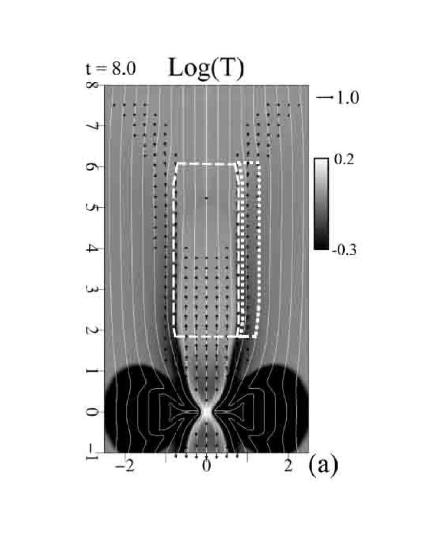
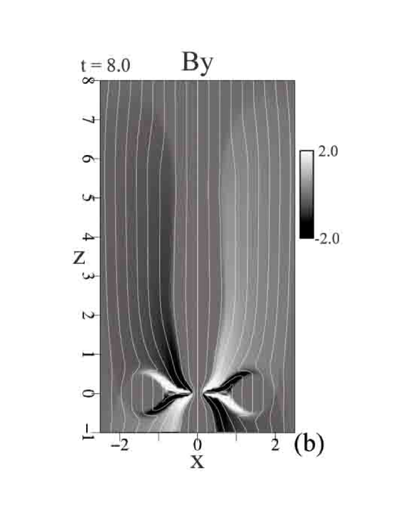
Figure 3: (a) The distribution of logarithmic temperature (gray-scale, dark is lower temperature) together with the poloidal field (white curves) and poloidal velocity field (arrows) in the $x-z$ plane. The white box with dotted lines, and that with dashed lines are assumed to be the Faraday rotation screen, and the emission region, respectively. (b) The poloidal magnetic field and the toroidal magnetic field ($B_{y}$) (gray-scale, white is plus and dark is minus).

Here we separate the Faraday rotation screen and the emitting region, and we performed the integrations only in the emitting region for the Stokes parameters, and only in the Faraday rotation screen for the FRM. We assumed this separation on the basis of the fact that linear dependence of the observed polarization angle on wavelength-squared holds in some observations (Perley, Bridle, & Willis 1984, Feretti et al. 1999, Asada et al. 2002); this would not be the case if the Faraday rotation is caused in the emitting region (Burn 1966). Figure 3 shows the emitting region (the region in the box of dashed lines) and the Faraday rotation screen (the region in the box of dotted lines) assumed in our calculations. The cylindrical shell outside the emitting region is assumed to play the main role of the Faraday rotation screen, because the temperature is lower and the toroidal field is stronger there (Figure 3) compared with those in the tenuous clouds in the intergalactic space.

We consider two types of the emitting regions; one is the layer type (type L: high energy particles exist only in the skin part of the dashed box in Figure 3(a)), and the other is the column type (type C: high energy particles fill the whole region of the dashed box). The former corresponds to the idea that the high energy particles are injected into the inner skin part of the jet due to the magnetic reconnection at the inner edge of the accretion disk as described in the previous section. The latter may happen if the high energy particles come from the pair plasma creation in the black hole magnetospheres.

4 Results of Numerical Observations

4.1 Faraday Rotation Measure

The model counterparts of the FRM distribution with different viewing angles are shown in Figure 4. When we see the jet from the direction perpendicular to its axis ($\theta=90^{\circ}$, $\theta$ is the angle between the jet axis and the line-of-sight), we see only the toroidal component of the helical field and thus the value of the FRM is almost antisymmetric with respect to the axis (it is not perfectly antisymmetric because the radial component of the magnetic field is not equal to zero). The distribution of the FRM is distorted from antisymmetry as the viewing angle varies, but it always shows gradient across the jet axis (Figure 4-2); this gradient across the jet axis can be interpreted as the sum of the antisymmetric part due to the toroidal component of the helical field and a base-value due to the longitudinal component. When $|\theta-90^{\circ}|$ is larger than the pitch angle of the helical field, this longitudinal component dominates (Figure 4-1).

4.2 Projected Magnetic Field and Total Intensity

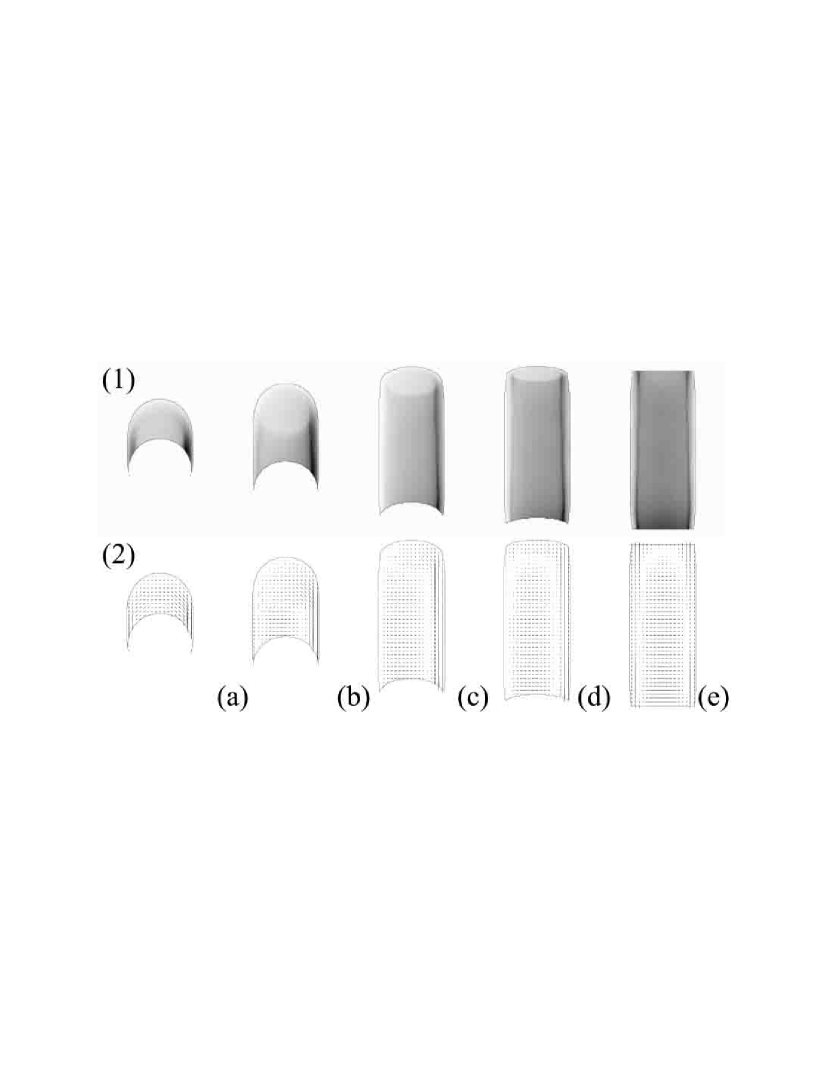
Figure 5: Calculated model counterparts for the total intensity and the projected magnetic field in the case of the type L emitting region, when seen at (a) $15^{\circ}$, (b) $30^{\circ}$, (c) $60^{\circ}$, (d) $75^{\circ}$, and (e) $90^{\circ}$, from the axis. The black in the gray scale indicates the maximum and the white indicates the minimum.

Figure 5 shows the distributions of the projected magnetic field and the total intensity with different viewing angles in the case of the type L emitting region. When $\theta$ is equal to $90^{\circ}$, the total intensity is nearly constant, but has an edge-brightening; this is because the emissivity becomes smaller away from the axis and the integration depth of the emitter has a maximum at edges. In other cases, the distribution of the total intensity is asymmetric, since the emissivity changes as $|\sin\left(\theta-\zeta\right)|^{\alpha+1}$ at the left edge and $|\sin\left(\theta+\zeta\right)|^{\alpha+1}$ at the right edge, where $\zeta$ is the pitch angle of the clockwise (seen from the jet origin) helical field. Therefore, for example, it becomes dark at the left edge when $\theta$ is nearly equal to $\zeta$. As for the projected magnetic field, it is perpendicular to the jet axis in the almost entire region, which does not depend on the viewing angle. This is because the the toroidal magnetic field is dominant in the emitting region.

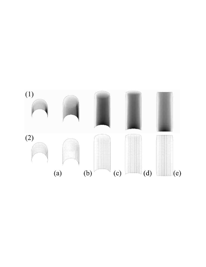
Figure 6: Calculated model counterparts for the total intensity and the projected magnetic field in the case of the type C emitting region, when seen at (a) $15^{\circ}$, (b) $30^{\circ}$, (c) $60^{\circ}$, (d) $75^{\circ}$, and (e) $90^{\circ}$, from the axis. The black in the gray scale indicates the maximum and the white indicates the minimum.

Figure 6 shows the distributions in the case of the type C emitting region. In this case, the intensity has the peak on the axis when $\theta=90^{\circ}$, because the integration depth has a maximum at the center of the jet. When the viewing angle is not so small, the projected magnetic field is parallel to the jet axis, which corresponds to the poloidal magnetic field in the emitting region. When the viewing angle is small (e.g. $\theta=15^{\circ}$), the distributions of the total intensity and the projected magnetic field are almost same as those in the type L. This is because the fraction of the magnetic field perpendicular to the line-of-sight, which contributes to the synchrotron radiation, is small in both cases.

5 Summary and Discussion

We calculated the FRM and the Stokes parameters using numerical data of 2.5-dimensional MHD simulation based on our “sweeping magnetic twist model”. The distribution of the FRM always has a gradient across the jet axis, which is caused by the toroidal magnetic field generated by the disk rotation. In calculating the Stokes parameters, we assumed two types of emitting regions, the column type and the layer type. In the former, the projected magnetic field tends to be parallel to the jet axis and the total intensity has the peak at the jet center. On the other hand, in the latter, the projected magnetic field is perpendicular to the axis; the total intensity has “edge-brightening”, which is observed in Centaurus A (Clarke, Burns, & Feigelson 1986), M87 (Biretta, Owen, & Hardee 1983, Junor, Biretta, & Livio 1999). In the following, we discuss the 3-dimensional magnetic field structure around the observed jets using these results of our numerical observations, especially focusing on the FRM distribution.

Figure 7 shows a recent observational result for 3C273 jet obtained by Asada et al. (2002) by using the VLBA Archive Data. In this case, the FRM distribution has a systematic gradient in the direction perpendicular to the jet axis, which can be interpreted as the sum of an antisymmetric distribution and a base value (a constant over the source). It is not likely that the foreground magnetized cloud at a large distance from the jet has a very sharp variation of either magnetic field or the density, just along the projected very thin jet (Taylor 1998, Asada et al. 2002). One likely interpretation may be that the antisymmetric contribution is due to the toroidal component of the helical magnetic field as stated in the above. The base-value may come either from the foreground large scale magnetized clouds at large distances, or from the longitudinal component of the helical magnetic field. The latest observation of the 3C273 jet shows that the systematic FRM gradient persists along a more significant length of the jet (Asada, private communication), which would be a strong evidence for the above idea.

The projected magnetic field in 3C273 is generally tilted somewhat from the axis of the jet, and the tilt angle becomes large at the blob called “anomaly”. Asada et al. (2002) attributed this to the shocks created on encountering non-uniformity. Another possibility is that the jet is bent at that point so that the jet axis has less angle from the line-of-sight; the change of the FRM value can be explained with our model counterparts of different viewing angles (see the change, for example, from (c) to (b) in Figure 4(1)).

The observation of the jet from the AGN core of NGC6251 (Perley et al. 1984) is shown in Figure 8. This may be a bit weaker evidence, but still considerably positive evidence for the systematic twist in the magnetic field. In this case, the contour lines of the FRM are nearly parallel in the central region up to 40″; therefore the distribution of the FRM has a systematic antisymmetry with a gradient in the direction perpendicular to the jet axis, if we subtract the possible contribution from the spherically condensed gas cloud probably associated with the central part of the host galaxy. The projected magnetic field is aligned and this would be consistent with the propagation of the torsional Alfvén waves.

The systematic and gradual change of the FRM value across the jet axis as seen in the above examples might suggest the existence of helical magnetic field. In the MHD models, it is naturally explained as the results of the interaction between the large-scale magnetic field and the disk rotation. Non-magnetic models may not be able to explain the FRM gradient. Although hydrodynamic models can include magnetic field as a passive ingredient, the magnetic field in such a case is expected to be carried around passively by the motions of non-magnetic gas dynamics. Such passively distorted magnetic field will produce the Faraday depolarization, rather than showing clear systematic FRM distribution.

The FRM distribution, when the Faraday rotation occurs in the external medium around the jet, can be useful to determine the 3-dimensional magnetic field structure around the jet, together with the projected magnetic field. We have demonstrated that the characteristic distribution of the FRM (systematic gradient perpendicular to the jet axis) in the straight part of some AGN jets can be explained by our “sweeping magnetic twist model”. On the basis of this success, we are extending our numerical observation to the wiggled part of jets, which can be explained as a structural helix produced by MHD kink instability in the regime of our model (Nakamura et al. 2001). The results will be reported in the following paper.

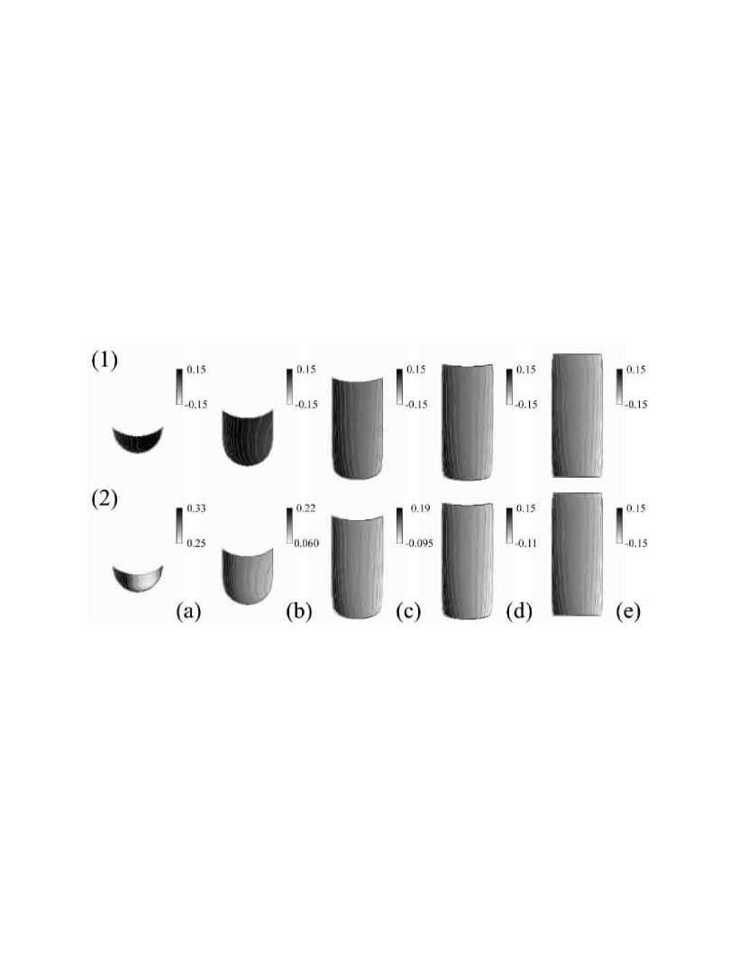
Figure 4: Calculated model counterparts for the FRM distribution, when seen at (a) $15^{\circ}$, (b) $30^{\circ}$, (c) $60^{\circ}$, (d) $75^{\circ}$, and (e) $90^{\circ}$, from the axis (ahead of the jet). Only those corresponding to the upper part of the jet ($z>0$) are shown. The direction of the jet coincides with that of the longitudinal magnetic field. The gray-scale range of the FRM distribution is fixed in the 1st row, while it is determined in each viewing angle in the 2nd row. The accretion disk is lower side in these pictures.

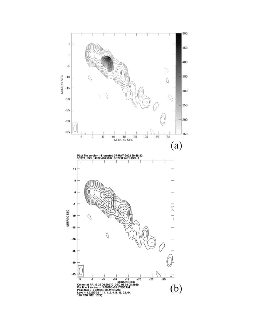
Figure 7: The distributions of (a) the Faraday rotation measure (this was modified from color picture to monochrome by courtesy of the authors), and (b) the direction of projected magnetic field, in the 3C273 jet (Asada et al. 2002).

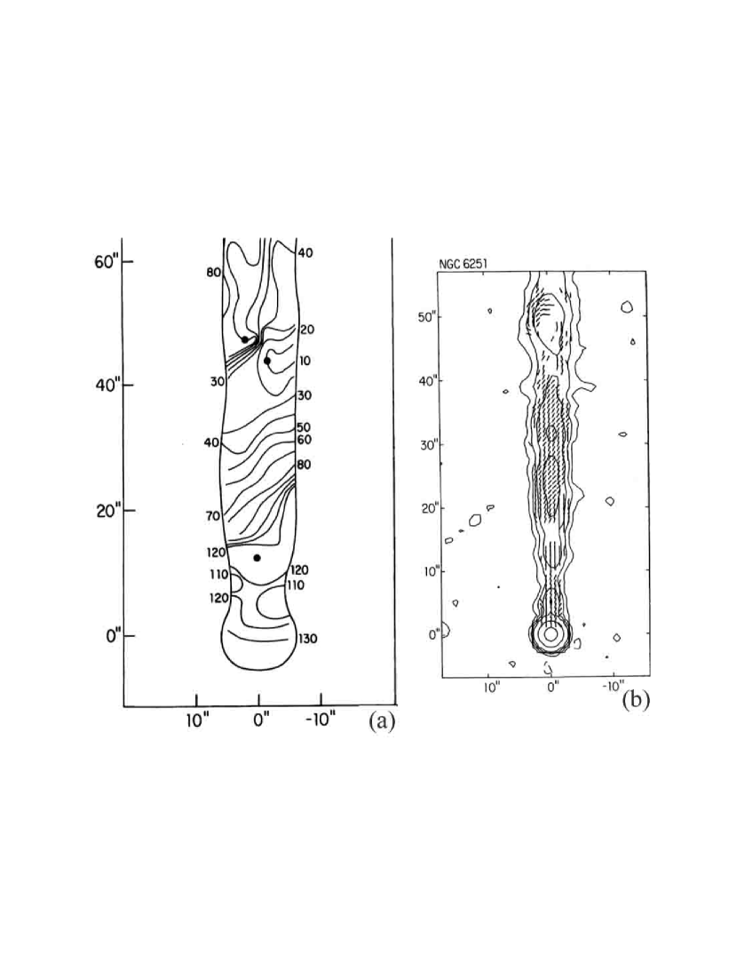
Figure 8: The distributions of (a) the Faraday rotation measure, and (b) the direction of projected magnetic field, in NGC 6251 jet (Perley et al. 1984).

References

- Asada et al. (2002) Asada, K., Inoue, M., Uchida, Y., Kameno, S., Fujisawa, K., Iguchi, S., & Mutoh, M. 2002, PASJ, 54, L39
- Biretta et al. (1983) Biretta, J. A., Owen, F. N., & Hardee, P. E. 1983, ApJ, 274, L27
- Blandford (1976) Blandford, R. D. 1976, MNRAS, 176, 465
- Blandford & Payne (1982) Blandford, R. D., & Payne, D. G. 1982, MNRAS, 199, 883
- Burn (1966) Burn, B. J. 1966, MNRAS, 133, 67
- Clarke et al. (1986) Clarke, D. A., Burns, J. O., & Feigelson, E. D. 1986, ApJ, 300, L41
- Clarke et al. (1989) Clarke, D. A., Norman, M. L., & Burns, J. O. 1989, ApJ, 342, 700
- Eilek & Owen (2002) Eilek, J. A., & Owen, F. N. 2002, ApJ, 567, 202
- Feretti et al. (1999) Feretti, L., Perley, R., Giovannini, G., & Andernach, H. 1999, A&A, 341, 29
- Hardee & Rosen (1999) Hardee, P. E., & Rosen, A. 1999, ApJ, 524, 650
- Hardee & Rosen (2002) Hardee, P. E., & Rosen, A. 2002, ApJ, 576, 204
- Junor et al. (1999) Junor, W., Biretta, J. A., & Livio, M. 1999, Nature, 401, 891
- Koide et al. (1998) Koide, S., Shibata, K., & Kudoh, T. 1998, ApJ, 495, L63
- Kudoh & Shibata (1997a) Kudoh, T., & Shibata, K. 1997a, ApJ, 474, 362
- Kudoh & Shibata (1997b) Kudoh, T., & Shibata, K. 1997b, ApJ, 476, 632
- Kudoh et al. (1998) Kudoh, T., Matsumoto, R., & Shibata, K. 1998, ApJ, 508, 186
- Laing (1981) Laing, R. A. 1981, ApJ, 248, 87
- Lovelace (1976) Lovelace, R. V. E. 1976, Nature, 262, 649
- Matsumoto et al. (1996) Matsumoto, R., Uchida, Y., Hirose, S., Shibata, K., Hayashi, M., Ferrari, A., Bodo, G., & Norman, C. 1996, ApJ, 461, 115
- Meier et al. (2001) Meier, D. L., Koide, S., & Uchida, Y. 2001, Science, 291, 84
- Nakamura et al. (2001) Nakamura, M., Uchida, Y., & Hirose, S. 2001, New Astronomy, 6, 61
- Ouyed & Pudritz (1997) Ouyed, R., & Pudritz, R. E. 1997, ApJ, 482, 712
- Perley et al. (1984) Perley, R. A., Bridle, A. H., & Willis, A. G. 1984, ApJS, 54, 291
- Stone & Norman (1994) Stone, J. M., & Norman, M. L. 1994, ApJ, 433, 746
- Taylor (1998) Taylor, G. B. 1998, ApJ, 506, 637
- Uchida & Shibata (1985) Uchida, Y., & Shibata, K. 1985, PASJ, 37, 515
- Uchida & Shibata (1986) Uchida, Y., & Shibata, K. 1986, Can.J.Phys., 64, 507
- Uchida et al. (1999) Uchida, Y., Nakamura, M., Hirose, S., & Uemura, S. 1999, Ap&SS, 264, 195
- Ustyugova et al. (1995) Ustyugova, G. V., Koldoba, A. V., Romanova, M. M., Chechetkin, V. M., & Lovelace, R. V. E. 1995, ApJ, 439, L39