Exploring spiral galaxy potentials with hydrodynamical simulations

Abstract

We study how well the complex gas velocity fields induced by massive spiral arms are modelled by the hydrodynamical simulations we used to constrain the dark matter fraction in nearby spiral galaxies (Kranz et al. 2001, 2003) . More specifically, we explore the dependence of the positions and amplitudes of features in the gas flow on the temperature of the interstellar medium (assumed to behave as a one-component isothermal fluid), the non-axisymmetric disk contribution to the galactic potential, the pattern speed, $\Omega_{\rm p}$ and finally the numerical resolution of the simulation. We argue that, after constraining the pattern speed reasonably well by matching the simulations to the observed spiral arm morphology, the amplitude of the non-axisymmetric perturbation (the disk fraction) is left as the primary parameter determining the gas dynamics. However, due to the sensitivity of the positions of the shocks to modeling parameters, one has to be cautious when quantitatively comparing the simulations to observations. In particular, we show that a global least squares analysis is not the optimal method for distinguishing different models as it tends to slightly favor low disk fraction models. Nevertheless, we conclude that, given observational data of reasonably high spatial resolution and an accurate shock-resolving hydro-code this method tightly constrains the dark matter content within spiral galaxies. We further argue that even if the perturbations induced by spiral arms are weaker than those of strong bars, they are better suited for this kind of analysis because the spiral arms extend to larger radii where effects like inflows due to numerical viscosity and morphological dependence on gas sound speed are less of a concern than they are in the centers of disks.

1 Introduction

Because gas responds strongly to nonaxisymmetries in a gravitational field, it was recognized more than two decades ago as a sensitive tracer of galactic potentials. Therefore, a model for such a potential can be tested by simulating the gas flow within it, and comparing the resulting morphology and kinematics to observations. The earliest efforts to apply such a method used general forms for the potential derived either from N-body simulations (Huntley 1978) or from analytic considerations (Sanders and Tubbs 1980). The parameters of these model potentials were then constrained by comparing results from hydrodynamical simulations performed with the beam scheme (Sanders and Prendergast 1974) to the morphology and kinematics of NGC 5383. The aim was to understand how the general features of the gas in a typical SBb(s) galaxy arose. Since NGC 5383 was being used as a representative of SBb(s) galaxies, Duval and Athanassoula (1983) recognized the importance of doing a careful observational study of it and hence obtained more complete spectral and photometric data for it. However using better data did not resolve the discrepancies between modeled and observed kinematics. They blamed it both on an inhomogeneity of the observations and an inadequacy of the models. Subsequent efforts to constrain disk galaxy potentials via hydrodynamical simulations have benefited from improvements in hydrocodes and have focused on deriving galactic potentials from specific galaxies rather than assuming a general form for them (England 1989, Garcia-Burillo, Combes & Gerin 1993, Sempere, Garcia-Burillo, Combes, & Knapen 1995, Sempere, Combes, & Casoli 1995, Lindblad, Lindblad and Athanassoula 1996, Lindblad and Kristen 1996, Sempere & Rozas 1997).

Interest in this approach has recently resurfaced with the defined goal of discerning the dark matter content of disk galaxies. For the case of barred galaxies, where gas motion in the inner region is strongly non-circular, with velocity gradients on the order of hundreds of kilometers a second, Weiner, Sellwood & Williams 2001 argued that model fits to the observed velocity fields could unequivocally differentiate between maximal and submaximal disks. With the same goal in mind, we undertook an investigation to break the disk-halo degeneracy in any spiral galaxy by studying the response of gas flow to the weaker perturbations induced by spiral arms. We began the study with the spiral galaxy NGC 4254 (Kranz, Slyz & Rix (2001, hereafter Paper I) and then applied the method to a sample of four additional high-surface brightness, late-type spiral galaxies (NGC 3810, NGC 3893, NGC 5676 and NGC 6643) (Kranz, Slyz & Rix 2003). To summarize, the studies were based upon the assumption that provided the dark matter halo is axisymmetric, all non-axisymmetric features observed in the velocity field of the gaseous disk have to be generated by the stellar mass component. Therefore, while completely smooth rotation curves do not betray any information about the dark and baryonic fractions of galaxies, non-axisymmetric features in rotation curves might break the baryonic/dark matter degeneracy.

We expected that when gas in our simulations would cross a spiral feature in the potential there would be a “wiggle” in the velocity field whose amplitude would be proportional to the local stellar mass fraction. Ideally, the simulated velocity wiggles would correlate well with those measured in the observed gas velocity field if the gravitational potential used for the simulations was derived from the observed mass distribution. However in modelling the gas flow in different galaxies we found that we could not account for every feature observed in the H$\alpha$ gas kinematics. The identifications of kinematical features in the simulations with those in the observations were often ambiguous. Kinematical features in the simulations sometimes appeared to be displaced, and/or to have a different profile, or amplitude.

Before considering the addition of more physics to our simulations, such as self-gravity or a multiphase interstellar medium sustained by star formation, supernovae and stellar winds, we propose in this paper to take a closer look at how the gas flow in a model of one of our sample galaxies, NGC 4254, changes as a function of our model parameters. More specifically, we investigate how much of the mismatch that we see is due to the coarseness of our parameter space exploration and how sensitive the positions, amplitudes, and profiles of features in the gas flow are to the parameters. In parallel, we also search for systematic measurements that can gauge the accuracy of a model potential. This allows us to estimate the numerical error associated with our simple hydrodynamical model, and therefore to assess the robustness of our result for the disk fraction of NGC 4254, namely that it is $\leq$ 85 per cent of its maximal value, implying that $\geq$ 1/3 of the total mass within 2.2 $K$-band disk scale length is dark (Paper I).

Hence, the paper is organized as follows. Section 2 gives a brief description of the hydrodynamical method we use and it introduces the parameter space we explore in this paper. It further describes the initial and boundary conditions of our models, addresses the question of whether the gas flow in our simulations reaches a quasi steady-state, explores the choice of the initial gas density profile and grid resolution. Section 3 proceeds to examine how the gas flow in the spiral potential depends on the modeling parameters, namely the contribution of the non-axisymmetric component to the galaxy potential, the gas sound speed and the potential’s pattern speed. Section 4 deals with the mass inflow as a function of the examined parameters and the hydrodynamical method. Section 5 gives our interpretation of the parameter study based on two different approaches to determine the quality of match between observations and simulations. Finally section 6 presents our conclusions.

2 Hydrodynamical Modeling

Our simulations are carried out using the BGK (Bhatnagar-Gross-Krook) hydrocode, a code based on gas-kinetic theory (Prendergast and Xu 1993, Slyz and Prendergast 1999). This is a high-resolution, Eulerian, grid-based hydrodynamics code. At each grid wall, BGK computes time-dependent hydrodynamical fluxes from velocity moments of a distribution function which is a local solution to a model of the collisional Boltzmann equation, namely the BGK equation. Because the BGK scheme evolves gas flow through an equation that includes particle collisions, the fundamental mechanism for generating dissipation in gas flow, the BGK flux expressions carry both advective and dissipative terms. If the grid is not fine enough to resolve a shock, then the collision time which is recomputed at each wall of the grid and with each timestep is enlarged to increase the viscosity and heat conduction at that particular location. Thereby even when the dissipation is put in for numerical reasons, it is added into the fluxes in exactly the same way that the physical dissipation is put into the code, hence there is no source term for either the physical or artificial dissipation. The code has been extensively tested on standard 1D and 2D test cases of discontinuous nonequilibrium flows (see Xu 1998 for a review). It has been used to solve Navier-Stokes problems in smooth flow regions both with (Slyz et al. 2002) and without (Xu and Prendergast 1994) gravity, and it has been tested for its long-term stability and convergence to the equilibrium solution in a fixed external gravitational field (Slyz and Prendergast 1999).

One reason for carrying out the disk simulations with this code, is its low diffusivity, a property that is critical not only to capture the shocks that form when the gas orbits in the non-axisymmetric potential, but also to properly model the loss of angular momentum and hence the resulting radial inflow of the gas due to the strong shear in the underlying differentially rotating disk. Slyz et al. (2002) showed that if an isothermal gas is initialized to be in centrifugal equilibrium within a purely axisymmetric galactic potential, simulation with the BGK scheme produces the steady-state Navier-Stokes solution to a high degree of accuracy. The tests were carried out for parameters which are relevant for galaxy studies: an asymptotically flat rotation curve with $v_{\rm max}=$ 220 $\,{\rm{\ }km{\ }s^{-1}}$ , a sound speed of $c_{\rm s}=$ 10 $\,{\rm{\ }km{\ }s^{-1}}$ , i.e. a highly supersonic (Mach $\approx$ 20) shear flow throughout most of the disk. The success of BGK in giving viscous radial flows on the order of 1 $\,{\rm{\ }km{\ }s^{-1}}$ in a disk rotating differentially at 220 $\,{\rm{\ }km{\ }s^{-1}}$ is a technical success which insures that when studying the kinematics of the gas in a galactic disk, with a decent grid resolution, one does not have to worry about artificial dissipation.

The number of grid cells, i.e. the spatial resolution of a simulation, is one of the parameters whose variation we study in this paper. In addition to the dissipation introduced by the BGK algorithm, there is the inevitable dissipation arising from the fact that the code only saves cell averages at the end of each iteration. Hence the larger the cells, the less information the code retains. To keep this numerical dissipation which is proportional to the cell dimensions at a constant value throughout the grid, we perform our simulations on an evenly spaced Cartesian grid. Our runs in Paper I were performed on a 201 $\times$ 201 grid giving a resolution element of about 115 pc on a side. For comparison, in this paper we look at runs done at half (101 $\times$ 101) and double that resolution (401 $\times$ 401).

There are three other parameters we explore in our modeling. As already stated in the introduction and described in Paper I, for our numerical investigation of the solutions for gas flow in the gravitational potential of NGC 4254 we use a potential derived from observations. The mass-to-light ratio corrected $K$-band image provides us with a stellar density map from which we compute the form of the non-axisymmetric component of the gravitational potential, and the rotation curves from observed long-slit H-alpha kinematics give us a measurement of the total gravitational potential of the galaxy. By assuming an axisymmetric isothermal profile for the dark halo we construct a series of potentials of different values for the strength of the stellar contribution, $f_{\rm d}$ (cf. eqns. 9 and 10, Paper I), which all match the observed rotation curve. Constraining the parameter $f_{\rm d}$ is our main scientific objective. Note that we do not work with a self-consistent model. We dynamically follow the gas, neglecting its self-gravity, in a fixed external potential which represents the combined gravitational effect of stars and dark matter.

Another parameter which plays the most important role in shaping the gas morphology in our simulations is the pattern speed, $\Omega_{\rm p}$, of the external potential. We assume the entire potential rotates rigidly with the same time-independent pattern speed and we perform the simulations in this rotating reference frame. We choose the direction of pattern and gas rotation to be clockwise so that inside corotation the gas enters the spiral arms from the concave side. Figure 1 shows how the locations of the resonances change with the different $\Omega_{\rm p}$ that we use.

We keep away from the difficult question of how the spiral formed, and we do not look for time-dependent solutions. Instead we study only steady or quasi-steady flows in NGC 4254’s fixed external gravitational potential. In the time-independent case, the gas flow must satisfy:

$$\vec{u}\cdot\nabla\vec{u}+2\Omega_{\rm p}\times\vec{u}=-\nabla p/\rho\pm\nabla\Phi$$ (1)

$$\nabla\cdot(\rho\vec{u})=0$$ (2)

where $\Phi$ is the potential of the combined centrifugal and gravitational forces. This system of equations must be completed by an equation of state and this introduces the last parameter of the problem: the gas sound speed. Because we do not know the effective equation of state of interstellar matter, the simplest thing to do is to assume an isothermal equation of state $p=K\rho$, where K $={c_{\rm s}}^{2}/\gamma$, $\gamma$ being the ratio of specific heats of the gas, and $c_{\rm s}$ is its constant sound speed. To study how the gas flow responds to changes in ${c_{\rm s}}$, we simulate the gas with sound speeds of 10, 15, 20 and 30 $\,{\rm{\ }km{\ }s^{-1}}$ .

Since the scale height of gas and stars in a typical non-interacting late type disk galaxy is about 1/40 to 1/75 the diameter of the visible galactic disk (e.g., Schwarzkopf & Dettmar 2000), we restrain this study to two-dimensions. More specifically we approximate the disk as a thin sheet, and only compute the gas flow in the two dimensions of the disk plane. Alternatively, one can view this approximation as an integration over the disk thickness perpendicular to the plane, and our physical variables as mean values in this direction.

Table 1 summarizes the parameters we use for the simulations and indicates the parameters of our fiducial simulation in boldface.

2.1 Initial conditions

We initialize the gas density profile to be exponential with a scale length which is on the order of the observed disk’s stellar scale length, namely 3.86 kpc. Upon estimating the total mass of the galaxy from the observed rotation curves, we set the mass of the gaseous disk to be 5 per cent of this total mass. The gas is therefore moving in a potential produced by a mass much greater than itself which means that, even in the densest regions (spiral arms), the neglect of its self-gravity will translate into a modest underestimate of its density (Berman, Pollard and Hockney 1979).

Figure 1: Plot of NGC 4254’s angular velocity $\Omega(R)$ (thick solid line) derived from an axisymmetric fit to its rotation curve. Overplotted are the angular velocities, $\Omega_{\rm p}$, of the different rigidly rotating reference frames which we explore (solid horizontal lines), and curves showing $\Omega-\kappa/m$ where m is 2 (dotted curves) and 4 (dashed curves).

Table 1: Specifications of the hydrodynamical simulations. Values for fiducial run given in boldface.

Simulation Parameters
grid length (kpc)	23.2
$\rm{v}_{\rm max}$ ($\,{\rm{\ }km{\ }s^{-1}}$ )	152
Initial Gas Mass	$3.14\cdot 10^{9}$${\rm M_{\odot}}$
number of grid cells	$101^{2}$,${\bf 201^{2}}$,$401^{2}$
time to turn on full potential ($\rm{t}_{\rm FP}$)	$20{\ }\rm{t}_{\rm s}$,$40{\ }\rm{t}_{\rm s}$,$80{\ }\rm{t}_{\rm s}$
time for entire simulation	$\rm{t}_{\rm FP}+2{\ }\rm{t}_{\rm dyn}$
gas sound speed ($\,{\rm{\ }km{\ }s^{-1}}$ )	10, 15, 20, 30
$\Omega_{\rm p}$ ($\,{\rm{\ }km{\ }s^{-1}}$ /kpc)	26.8, 19.9, 18.3, 15.2
${\rm R}_{\rm c}$ (kpc) (corotation radius)	5.6, 7.58, 8.5, 10
${\rm f_{\rm d}}$ disk fraction (%)	20, 44, 60, 85, 100

Figure 2: The axisymmetric potential subtracted from the potential of NGC 4254. Contours are shown on the left with the force vectors, computed from the difference in the two potentials, overplotted. A filled contour plot is shown on the right, with the peaks of the potential given in white and the valleys in black.

As for the initial dynamics of the gaseous disk, the simulations begin with the gas flowing on circular orbits in inviscid centrifugal equilibrium with respect to the axisymmetric gravitational potential which best fits the observed rotation curves. The non-axisymmetric perturbations are then gradually turned on to avoid transient structures (Sorensen & Matsuda 1982). The criteria for the time in which the full potential is turned on, ($t_{\rm FP}$), is based on the sound crossing time across the diagonal of a grid cell ($t_{\rm s}$). For the 201 $\times$ 201 grid, we set $t_{\rm FP}=40{\ }t_{\rm s}$. Since the sound crossing time depends on the length of the grid cell, and for comparison’s sake we want $t_{\rm FP}$ and the total running time of each simulation to be identical, this implies $t_{\rm FP}=20{\ }t_{\rm s}$ for the 101 $\times$ 101 grid, and $t_{\rm FP}=80{\ }t_{\rm s}$ for the 401 $\times$ 401 grid. In terms of the dynamical time of the outer edge of the disk (${\rm t}_{\rm{dyn}}=\frac{2\pi R_{\rm{disk}}}{V_{c}}\approx$ 480 Myr for a rotational velocity of about 152 $\,{\rm{\ }km{\ }s^{-1}}$ at ${\rm R}_{\rm{disk}}=11.6$ kpc), for the case where the sound speed is 10 $\,{\rm{\ }km{\ }s^{-1}}$ and the grid is 201 $\times$ 201, this means that we turn on the full potential in 1.3 ${\ }{\rm t}_{\rm{dyn}}$. After the full potential is turned on, we continue to run the simulations for another two dynamical times. Figure 2 shows the non-axisymmetric component of the gravitational potential of NGC 4254 displayed on the 201 $\times$ 201 grid.

Figure 3: Contour maps showing three time steps separated by a Gyr of the simulated gas density for our fiducial run in order to demonstrate that the gas flow reaches a steady-state. The shaded plot in the lower right hand corner shows the density as a function of the azimuth along a circle of radius $R=3.8\,\rm{kpc}$ (indicated by a thick solid line on the contour plot at 3 Gyr) as a function of time. The solid vertical line in this plot indicates the time, $\rm{t_{\rm FP}}$, at which the full potential is turned on in the simulation. After $\rm{t_{\rm FP}}+\rm{t_{\rm dyn}}$ ($\approx 1.1$ Gyrs) the simulation yields a very stable pattern.

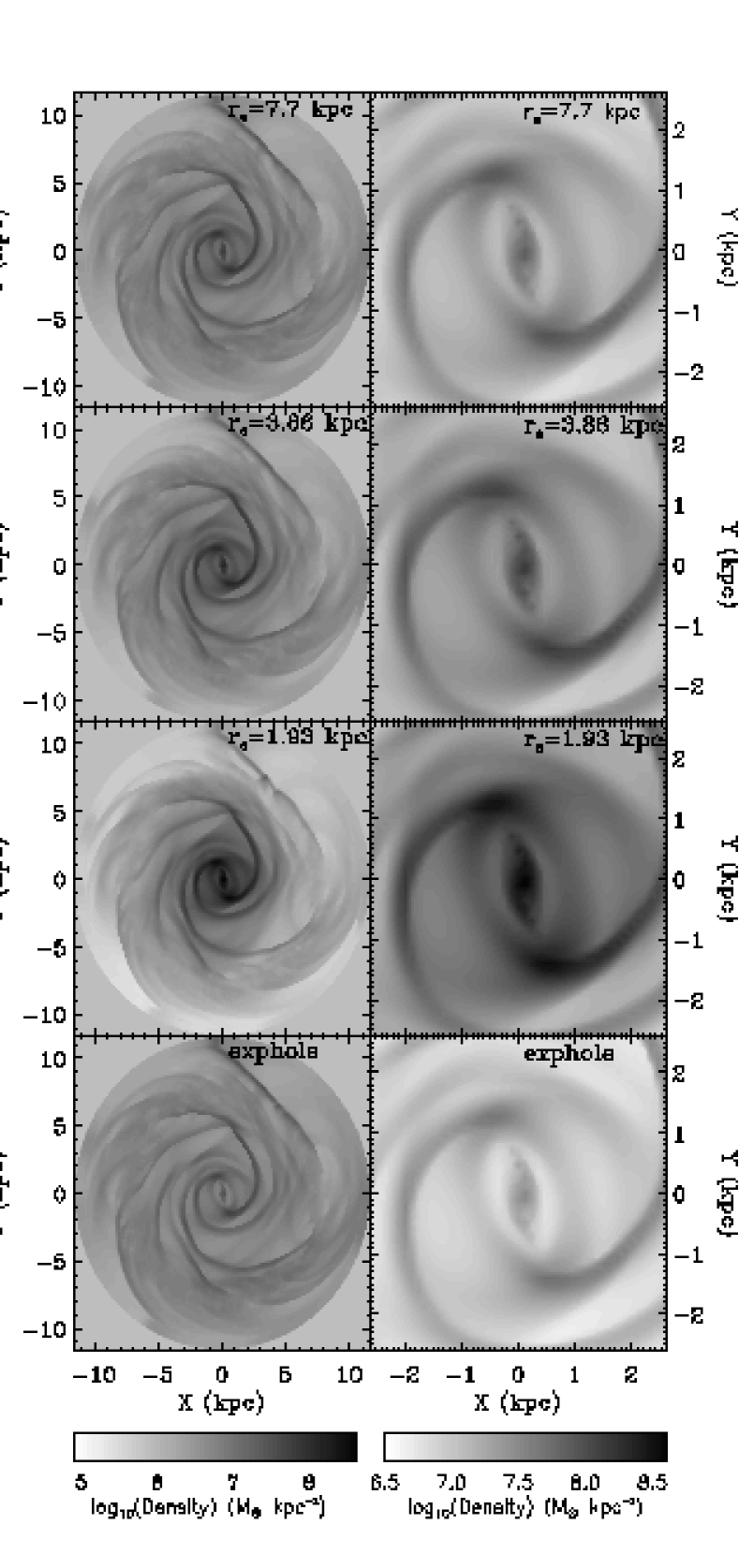
Figure 4: Grey scaled maps of the log of the density from simulations with our fiducial parameters and with different initial gas density profiles. The entire simulated region is shown in the left column and the inner 2.6 kpc² region is shown in the right column.

Figure 5: Natural logarithm of the average density (top panel) and density averaged radial velocity (bottom panel) at time $t=\rm{t}_{\rm FP}+2{\ }\rm{t}_{\rm dyn}\approx$1.6 Gyr for runs differing only in their initial density profile. The other parameters in the simulation are the fiducial ones.

2.2 Boundary conditions

Since we perform our computations on a Cartesian grid, the center of the disk (r = 0) is not a singular point, and therefore does not require special treatment via an inner boundary condition. Instead, the gas flow is computed through this point exactly as it is computed throughout the grid.

An outer boundary condition is, however, unavoidable. To tackle this issue, we keep two “rings” of one cell thick ghost cells outside of a radius of $R_{\rm disk}$. Beyond these ghost cells we do not follow the evolution of the gas. Hence we have effectively carved a circular grid out of the square Cartesian grid. At the end of each simulation timestep we update the values of the hydrodynamic quantities (mass, momentum and energy) in the ghost cells by performing a bilinear interpolation to the cells in the vicinity of the ghost cell. To be more specific, for each ghost cell in the inner ring for example, we compute the coordinates of the intersection of the line extending radially from the center of the disk to the ghost cell with the circle bounding the true flow region of the grid. We then find the four cells surrounding this intersection (some of which might be other ghost cells). After fitting a surface to the hydrodynamic quantities in these four cells we assign the ghost cell the value the fitted surface has at the intersection. By filling up the ghost cells via constant radial extrapolation that varies azimuthally around the disk, we are better able to handle situations in which there is a significant non-axisymmetry near the outer boundaries. For example, from the map of NGC 4254’s potential (Figure 2), one can see that the potential is quite non-axisymmetric near the upper boundaries thereby requiring an outer boundary condition which can take into account the possiblity that the flow in the outer regions of the disk may also be non-axisymmetric.

For the sake of completeness, we point out that we apply this boundary condition procedure directly to the mass densities. For the velocities, we take the additional steps of converting the Cartesian velocity components back to the non-rotating frame, then constructing the radial and tangential components of the velocity from the Cartesian components, and performing the bilinear interpolation and radial extrapolation procedure on these components. By performing the interpolation and extrapolation on the radial and tangential components in the non-rotating frame, we first set the boundary conditions for quantities that are easier to interpolate and extrapolate: namely the tangential velocity which is nearly flat (constant in x and y) and the radial velocity which is nearly zero in the disk’s outer regions in the nonrotating frame.

We stress that our boundaries allow gas flow across them. For different runs, mass loss/gain after about 1 $\rm t_{\rm dyn}$ ranges from $\approx$ 2 per cent for runs performed in the non-corotating frame or slowly corotating frames, to at most $\approx$ 15 per cent for the fastest corotating frame we simulated, i.e. when corotation is at $\approx$ 5 kpc.

2.3 Steady State ?

Before proceeding to an examination of how different physical parameters change the gas’ response to the underlying gravitational potential, we consider the question of whether our conclusions depend on the specific snapshot in time for which we analyze the simulation. For this we look at (fig. 3) the long term evolution of our “fiducial” model for NGC 4254. Displayed are the density contours at times 1, 2, and 3 Gyr. In terms of dynamical time, this corresponds to 2.1 $\rm t_{\rm dyn}$, 4.2 $\rm t_{\rm dyn}$, and 6.4 $\rm t_{\rm dyn}$. We see that the density field adjusts to the force input within a couple of dynamical times. Therefore, our simulations are even applicable to spiral arms which are not long-lived features, i.e. with ($t\approx t_{\rm dyn}$). To illustrate the steadiness of the features in time, we present a greyscale plot (lower right hand corner of figure 3) of the density as a function of both time and azimuth along a circle of $\approx$ 3.8 kpc radius (indicated by a thick solid line in the contour plot at 3 Gyr). The solid vertical line in the greyscale plot indicates the time at which the full potential is turned on in the simulation, i.e. $\rm t_{\rm FP}\approx$ 1.3 $\rm t_{\rm dyn}\approx$ .62 Gyr. Shortly after this moment (about 0.5 Gyr later), the morphology of the density distribution becomes nearly time-independent. The contour plots show that even the orientation of the very inner region which we are not trying to model in detail since it may have a different pattern speed from the outer spiral pattern, seems to be steady in time. What is true for the densities applies also to the velocities. They also reach a near steady state (cf. Fig. 6.3, Kranz 2002).

2.4 Influence of Initial Density Profile

To confirm that a specific choice of initial gas density profile does not introduce a bias in our study, we perform simulations with initial density profiles of double (7.72 kpc) and half (1.93 kpc) our fiducial initial scalelength of 3.86 kpc, as well as with an initial density profile which has a “hole” in the central region ($\rho_{\rm 0}(1+\frac{r}{r_{\rm c}})\exp(-\frac{r}{r_{\rm s}})$, where $r_{\rm c}=\rm 4.46$ kpc and $r_{\rm s}=\rm 7.72$ kpc). Figure 4 and the top panel of figure 5 reveal that while the density contrast depends on the initial density profile, the morphology of the final gas distribution is almost unaffected. The bottom panel of figure 5 further shows that the density averaged radial velocity is also very nearly independent of the initial density profile, except in a small region centered around the corotation radius (in this case $R_{\rm c}=7.58$ kpc). Note however that even in this region differences between models are slight.

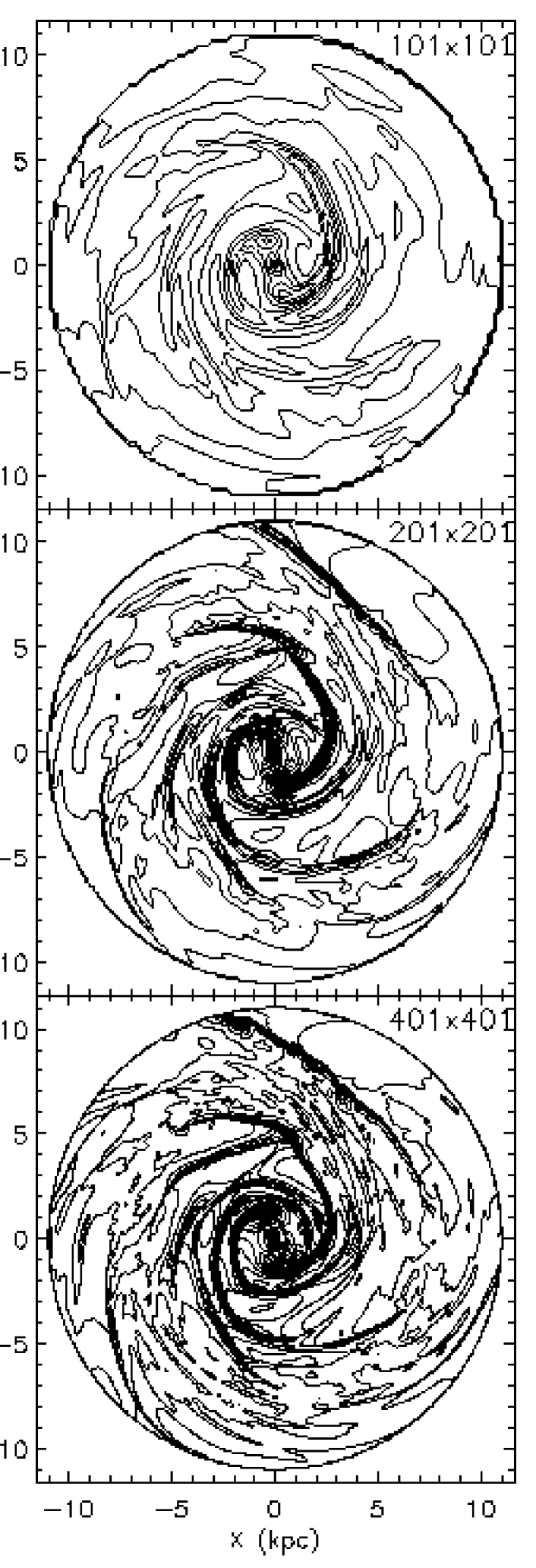
Figure 6: Contour maps of the density from simulations with $c_{\rm s}=10$ $\,{\rm{\ }km{\ }s^{-1}}$ , 60 per cent disk fraction, $R_{\rm c}=7.58$ $\rm{kpc}$, and with increasing grid resolution. The full potential is turned on in 20 cell sound crossing times for the 101 $\times$ 101 grid, 40 $t_{\rm s}$ for the 201 $\times$ 201 grid, and 80 $t_{\rm s}$ for the 401 $\times$ 401 grid. The result is shown after 1590 Myr ($\sim$ 3.3 $t_{\rm dyn}$) have elapsed.

Figure 7: The gas density and amplitude of the velocity as a function of azimuth for $R\approx$ 3 kpc, for simulations performed with $f_{\rm d}=60$ per cent, $R_{\rm c}=7.58$ $\rm{kpc}$, $c_{\rm s}=10$$\,{\rm{\ }km{\ }s^{-1}}$ and different grid resolutions.

2.5 Resolution

Results from any numerical study are also subject to the choice of grid resolution. Paper I was based on simulations performed with an evenly spaced grid of 201 cells in x and in y of length $\approx$ 115 pc per cell. Such a resolution quite closely matched the observed kinematics obtained from the long-slit spectra. Here, we run experiments using a grid with half and double this number of cells. We find that results have fairly well converged for the 201 $\times$ 201 grid. A plot of the density over the entire x-y plane, figure 6, for the sequence of increasing grid resolutions shows that the simulation performed on the 101 $\times$ 101 grid is missing many of the features present in the simulations on the 201 $\times$ 201 and the 401 $\times$ 401 grids.

More detailed examination of gas profiles in plots of the radial density profile for $\vartheta=202.5^{\circ}$ (figure 9) and of the azimuthal density profile for $r\approx$ 3 kpc (figure 7) reveals that the amplitudes of the density maxima for the 201 $\times$ 201 grid have nearly converged to their values on the 401 $\times$ 401 grid. There are however noteable differences between the profiles on the different resolution grids. Firstly, the phases of the density maxima are fairly well matched for the strong density maxima but less so for the lower density contrast ones. For example, as shown near $R\approx 6$ kpc on figure 9 higher resolution simulations tend to shift small density maxima to larger radii. Secondly, as can be seen on figs. 7 and 9, the shape of the density and velocity profiles changes with resolution. The lowest resolution grid yields the smoothest and most symmetrical gas profiles. However with a grid resolution of 201 $\times$ 201 one already recognizes the characteristic profiles described analytically by Roberts (1969). The profiles are asymmetric with a rapid density rise followed by a gradual decline (see fig. 7).

Interestingly, even though the numerical viscosity increases with lower grid resolution, implying higher numerical gas inflow into the center, we find that the density at $r=0$ for the 101 $\times$ 101 grid (figure 9) is actually lower than the central densities of the higher resolution simulations. We will discuss this result in more detail in section 4 but conclude here that the numerical errors associated with a 201 $\times$ 201 grid represent an $\approx$ 10 % contribution to the shape, amplitude, and position of the features of our discs.

3 Parameter Study

Following these considerations about resolution, initial conditions and the attainment of a quasi-steady state in the simulation, we focus on how the nature of gas flow in the potential is effected by changes in the three parameters enumerated in section 2: the amplitude of the disk contribution to the potential $f_{\rm d}$, the gas temperature $c_{\rm s}$, and the pattern speed $\Omega_{\rm p}$. We explore only variations in each of these three parameters individually, keeping the other ones fixed at their fiducial values (given in boldface in Table 1).

3.1 Different Disk Fractions

At first we examine how increasing the non-axisymmetric stellar mass component of a gravitational potential influences the simulated gas density distribution and the velocity field. The total potential, $\Phi_{\rm{tot}}$, was assembled in the following way:

$$\Phi_{\rm{tot}}({\bf R}\mid f_{\rm d})=f_{\rm d}\Phi_{\rm{stellar}}({\bf R})+\Phi_{\rm{halo}}({\bf R}\mid f_{\rm d})$$ (3)

adopting the values 0.2, 0.45, 0.6, 0.85 and 1 for $f_{\rm d}$. $\Phi_{\rm{stellar}}$ is the stellar potential with the maximal stellar mass-to-light ratio and $\Phi_{\rm{halo}}$ is the potential of the dark halo which is constrained by the observed rotation curve. For a fair comparison, all the simulations in this series of increasing disk fraction were run for the same amount of total time, namely $\sim$ 1.6 Gyr.

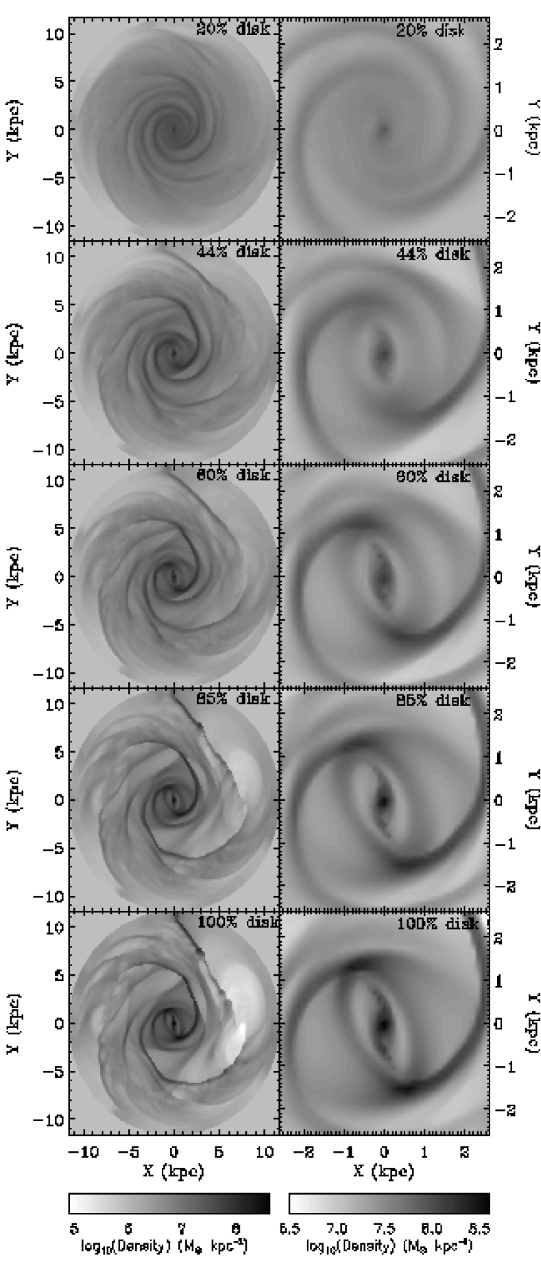
Figure 8: Grey scaled maps of the log of the gas density from simulations on a 201 $\times$ 201 grid, with $c_{\rm s}=$ 10 km $\rm{s}^{-1}$, and $R_{\rm c}=$ 7.58 $\rm{kpc}$, and with increasing disk contribution to the total galactic potential. The left column shows the entire simulated region, and the right column shows only the inner 2.6 kpc² region.

Figure 9: Cuts along an azimuth of $\vartheta=\rm 202.5^{\circ}$ of the log of the density for runs with $R_{\rm c}=$ 7.58 $\rm{kpc}$. Top panel shows results from a simulation performed on a 201 $\times$ 201 grid with $c_{\rm s}=10$$\,{\rm{\ }km{\ }s^{-1}}$ and varying disk fraction. Middle panel shows results from a simulation on a 201 $\times$ 201 grid, with a disk fraction of 60 per cent and varying sound speed. Lower panel shows results from a run with 60 per cent disk fraction, a sound speed of 10 $\,{\rm{\ }km{\ }s^{-1}}$ , and varying grid resolution. Each curve is displayed for the simulation at time $t=\rm{t_{\rm FP}}+2{\ }\rm{t_{\rm dyn}}$ ($\approx 1.6$ Gyrs).

A logarithmic plot (figure 8) of the gas density for the sequence of simulations, shows that the density contrast of the non-axisymmetric features in the gas increases as the disk fraction increases. This corroborates Figure 21 in this paper and Figure 8 of Paper I which quantified this trend by taking the average of the amplitude of the velocity deviations from axisymmetry, and found that this average increases more or less linearly with the disk fraction. In addition to the change in the density contrast, figure 8 shows that features become more “angular” with increasing disk fraction. For example, in the lowest disk fraction case (20 per cent disk), the spiral arms appear to be rounded and smooth in their curvature. As the disk fraction is increased to 85 per cent, the lower spiral arm develops a squareness which is even more pronounced for the 100 per cent disk fraction case.

To display these changes in amplitude and morphology in more detail, figure 9 plots the density profile along an azimuthal cut through the disk at a position angle $\vartheta=\rm 202.5^{\circ}$. The top panel of this figure shows that the smaller amplitude density peak (lower spiral arm) located at $R\approx$ 6 kpc moves outwards with increasing disk fraction suffering larger shifts in position with changing disk fraction than the larger amplitude peaks at smaller radii ($R<$ 2 kpc). To further quantify this, we plot the gas density and velocity amplitude as a function of azimuth for $R\approx$ 3 kpc (figure 10). In agreement with Woodward’s (1975) analytic calculations (his figure 7), we find that the location of the density peak moves towards larger azimuths with increasing perturbation strength. Figure 9 also indicates that as the disk fraction increases, regions of increasingly lower gas density appear immediately adjacent to the gas density peaks in the arms. Hence to differentiate between models with different $f_{\rm d}$ a code has to perform well in the low density regions, which is one of the strengths of grid codes over particle codes in general and of the BGK scheme in particular.

Figure 10: The gas density and amplitude of the velocity as a function of azimuth for $R\approx$3 kpc, for simulations performed on a 201 $\times$ 201 grid with $c_{\rm s}=10$$\,{\rm{\ }km{\ }s^{-1}}$ , $R_{\rm c}=7.58\rm{kpc}$ and different values for $f_{\rm d}$.

Figure 11: Cuts along different position angles of the difference between the velocity amplitude for runs with different disk fractions compared to a ’fiducial’ run with a 60 per cent disk fraction. All simulations referred to in this plot are done on a 201 $\times$ 201 grid, with a sound speed of 10 km $\rm s^{-1}$ and $R_{\rm c}=7.58$ kpc. The dash-dot-dot-dot line is for the 20 per cent disk, the dotted line is for the 44 per cent disk, the dashed line is for the 85 per cent disk and the dash dotted line is for the 100 per cent disk.

Morphological changes with increasing disk fraction are not limited to spiral arms: they are also present in the inner region of the galaxy. Even at the resolution of our study, the grey-scale maps of the inner regions of the disk (right column of figure 8), reveal the development of off-axis shocks, the emergence of an oval ring around the inner region, and the strengthening of the 4/1 shock at the endpoints of this oval ring.

Since we are ultimately comparing the kinematical information in the simulations to observations in order to constrain the dark matter fraction of the galaxy, we plot in figure 11 the difference between velocity amplitudes ($\sqrt{{v_{x}}^{2}+{v_{y}}^{2}}$) measured in each model and those measured in our fiducial run ($\rm f_{\rm d}=60$ per cent) along four position angles ($\vartheta=\rm 135^{\circ},\rm 180^{\circ},\rm 225^{\circ},\rm 270^{\circ})$. As already seen in figures 8,  9 as well as in figure 7 of paper I, there are significant variations in the models depending on the assumed value for $\rm f_{\rm d}$. The additional information contained in figure 11 is that changing $\rm f_{\rm d}$ has a greater impact on the central region of the disk where the differences in velocities between different models can reach 70 $\,{\rm{\ }km{\ }s^{-1}}$ . However there are also large velocity variations (10 - 40 $\,{\rm{\ }km{\ }s^{-1}}$ ) throughout the rest of the disk.

Another feature which reacts to the changing disk fraction is the shock touching the boundary in the upper right hand quadrant. It becomes more inclined towards the center of the disk and increases in length with increasing $\rm f_{\rm d}$, raising the concern that it might interact with other features in the disk. It is hard to discount this shock as artificial because Figure 2 indicates that there is a minimum in the potential in the upper quadrants of the grid. However it is likely that whatever structure forms in that area of the grid, may be affected by the outer boundary conditions.

3.2 Different Sound Speeds

Figure 12: Grey scaled maps of the log of the density from simulations on a 201 $\times$ 201 grid, with 60 per cent disk fraction, $R_{\rm c}=$ 7.58 kpc, and with increasing sound speed. The entire simulated region is shown in the left column and the inner 2.6 kpc² region is shown in the right column.

Figure 13: The gas density and amplitude of the velocity as a function of azimuth for $R\approx$3 kpc, for simulations performed on a 201 $\times$ 201 grid with $f_{\rm d}=60$ per cent, $R_{\rm c}=$ 7.58 kpc and different values for $c_{\rm s}$.

Figure 14: Cuts along different position angles of the difference between the velocity amplitude for runs with different sound speeds compared to a ’fiducial’ run with a sound speed of 10 km s^-1. All simulations referred to in this plot are done on a 201 $\times$ 201 grid, with a disk fraction of 60 per cent and $R_{\rm c}=$7.58 kpc. The dash-dot-dot-dot line is for $c_{\rm s}=15$$\,{\rm{\ }km{\ }s^{-1}}$ , the dotted line is for $c_{\rm s}=20$$\,{\rm{\ }km{\ }s^{-1}}$ , and the dashed line is for $c_{\rm s}=30$$\,{\rm{\ }km{\ }s^{-1}}$ .

Because it is thought that the interstellar cloud medium can be crudely approximated by an isothermal gas if the clouds have an equilibrium mass spectrum (Cowie 1980) maintained by supernovae which both destroy and create gas clouds, most simulations of gas flows in disk galaxies treat the gas as isothermal where the sound speed represents the rms velocity of the interstellar clouds. Simulations treating the gas as multi-phase are starting to be run (Colina & Wada 2000, Wada & Koda 2001, Slyz et al. 2003). Given the caveats in modeling a multi-phase interstellar medium, we find it prudent to keep the simple assumption of a uniform ISM for these global disk simulations, since, as already remarked in the Introduction, for our study in Paper I we are trying to match velocity wiggles in the observations to those in simulations in as much detail as possible. As a matter of fact it is virtually impossible to model star formation and feedback processes in our simulations in such a way as to match the velocity wiggles in the velocity spectra. In other words, our working hypothesis is that these wiggles arise from variations in the gravitational potential and therefore that an isothermal equation of state is a good description of the ISM. We are then left with examining the effect on our results of different assumptions for the uniform sound speed of the gas.

Typically authors assert that their hydrodynamical calculations are insensitive to reasonable changes in the sound speed (Lindblad, Lindblad, & Athanassoula 1996, Lindblad & Kristen 1996, Weiner et al. 2001). Given that flow velocities of the gas relative to the bar and/or spiral pattern greatly exceed the velocity dispersion of the interstellar medium throughout almost the entire disk of a galaxy, it indeed seems reasonable to think that there should be no strong dependence of the flow on the sound speed. At larger values of the sound speed ($\approx$25 km s^-1) however, detailed investigations of gas flows in strongly barred galaxies (Englmaier & Gerhard 1997; Patsis & Athanassoula 2000), show that the structure of the flow changes markedly.

The first effect of increasing the sound speed that one expects to find is that the gas should respond less strongly to the forcing pattern, since at higher sound speeds the pressure of the gas starts to become more important. This effect is evident in figure 12 where in a sequence of simulations differing only in their sound speed we see the non-axisymmetric features in the gas gradually fade with increasing sound speed. By $c_{\rm s}=30$ km s^-1 the spiral structure does not extend as far as it does in the colder gas runs even though traces of some of the larger spiral features are still present. We emphasize that sound speeds of 25 or 30 km s^-1 throughout the entire disk are unrealistically high. Results from simulations at these high values are merely included to illustrate trends of increasing sound speeds.

A close-up view (right hand column of figure 12) of the interior region of the simulation shows even more striking morphological differences between simulations at different sound speeds. Firstly we notice that the prominent spiral arm on the right side of the galaxy winds up more tightly with increasing sound speed. Secondly we see that the spiral arms reach further and further into the center of the disk until by $c_{\rm s}=$ 30 km s^-1 they are completely connected to the centermost region. The last principle morphological change we see is that the 4/1 shocks fade with increasing sound speed until they vanish by 25 km s^-1. Although the gravitational potential we are working with is different from the one used by Englmaier & Gerhard (1997) and Patsis & Athanassoula (2000), some of these changes that we see, namely the disappearance of the off-axis shocks and the fading of the 4/1 shocks, are similar to those they describe.

For a more detailed view of the influence of changing sound speed on the gas flow, we display the density profiles for the different runs at $\vartheta=\rm 202.5^{\circ}$ (figure 9). As expected the density profile for the simulation at $c_{\rm s}=$ 30 km s^-1 is everywhere much smoother than the density profiles for the other simulations. The density maximum in the middle of the disk ($R\approx 4-5$ kpc) is present for all the runs but it progressively shifts radially inwards with increasing sound speed which is a manifestation of the stronger winding of the spiral structure for larger sound speeds that was already mentioned above. Features between 2 and 3 kpc which are present for $c_{\rm s}=10$ km s^-1 are essentially gone by $c_{\rm s}=$25-30 km s^-1. Another effect seen in this figure, is that at $r=0$, the simulations with sound speeds between 10-20 km s^-1 achieve effectively the same density, but the density for the run with $c_{\rm s}=30$ km s^-1 is higher by a factor of $\approx 1.09$ in log-space.In a similar way as in figure 10 for the disk fractions, we plot the gas density and amplitude of the velocity for changing sound speed in figure 13. The density peak is systematically shifted towards larger azimuths for increasing sounds speeds again reflecting a tighter winding of the spiral, with a shift of $\approx 20^{\circ}$ between the smallest (10 km s^-1) and largest (30 km s^-1) sound speed we considered which is larger than the $15^{\circ}$ shift induced by changes in $f_{\rm d}$. However changing the disk fraction from 20 per cent to 100 per cent results in a difference of 53 $M_{\odot}$ $\rm{pc}^{-2}$ in density amplitude, as compared to a difference of 16 $M_{\odot}$ $\rm{pc}^{-2}$ for a variation in sound speed between 10 and 30 km s^-1. Thus the simulations are less sensitive in this respect to a change in $c_{\rm s}$ as compared to changes in $f_{\rm d}$.

Figure 14 shows the difference between velocity amplitudes for runs with different sound speeds compared to the run with $c_{\rm s}=10$ $\,{\rm{\ }km{\ }s^{-1}}$ , for the same four position angles used in figure 11. As was the case for the different $f_{\rm d}$ models, changing the sound speed has the greatest impact on the centermost region of the galaxy with velocity variations of up to $\approx$ 40 km s^-1. This is worrisome because it is similar to the variation in this region between the models for different disk fractions . However, if one excludes the centermost region of the disk, then variation in the velocity amplitudes as one changes the sound speed is much lower than the variations between the models for different disk fractions (at most $\approx 15$ km s^-1 as compared to $\approx 40$ km s^-1) This lower sensitivity to changes in sound speed in the face of uncertainties in how to model the interstellar medium, suggests that the gas response in the outer regions, as opposed to the inner regions, of the disk may more reliably trace the gravitational potential. Furthermore since a sound speed of 10 km s^-1 for the interstellar medium is physically motivated, we maintain that for simplicity’s sake, it is a good choice for these kind of studies.

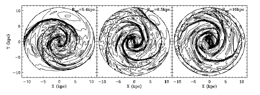
Figure 15: Density contours for 3 simulations differing in their pattern speed. The value for the corotation radius is marked in the upper right hand corner. All the simulations are performed for a model with 60 per cent disk fraction, $c_{\rm s}=10$ km s^-1 and on a 201 $\times$ 201 grid.

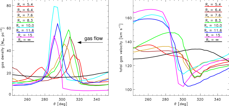
Figure 16: The gas density and amplitude of the velocity as a function of azimuth for $R\approx$3 kpc, for simulations performed on a 201 $\times$ 201 grid with $c_{\rm s}=10$$\,{\rm{\ }km{\ }s^{-1}}$ , $f_{\rm d}=60$ per cent, and a range of values for $R_{\rm c}$.

3.3 Different Pattern Speeds

Bar simulations have already shown that the most significant parameter in controlling the structure of the gas flow in a disk is its angular pattern speed, $\Omega_{\rm p}$ (e.g. Hunter et al. 1988). Given this sensitivity of the gas morphology to the pattern speed (see figures 15 and 16), matching the simulated density to an observation of the galaxy surface density may be a powerful way to constrain it (see e.g. Garcia-Burillo et al. 1993, Garcia-Burillo et al. 1994, Sempere et al. 1995, Mulder & Combes 1996, Paper I).

To elaborate, simulations in a fixed gravitational potential show that one of the things that the pattern speed and hence the corotation radius determines is the radial extent of the spiral pattern in the gas. This is easy to understand because the corotation radius is the radius at which the pattern speed $\Omega_{\rm p}$ is equal to the orbital frequency $\Omega$. Hence at the corotation resonance (see figure 1) the gas rotates along with the spiral perturbations and therefore the non-axisymmetric forcing vanishes. This causes spiral disturbances to be highly damped at corotation (see figure 15 for three cases of $\Omega_{\rm p}$). Outside corotation the spiral structure may resume. In light of this, it is expected (Shu, Milione & Roberts 1973) that at the corotation radius star formation cannot get excited by the density wave and should not be observed in a quiescent galaxy. Our best matching simulation for NGC 4254 (see Paper I) is consistent with this signature for corotation. It gave a corotation radius beyond which star formation, i.e. the occurrence of H II regions, was largely reduced.

Nevertheless, a major caveat of both this approach for determining the pattern speed, and of our assumption of a single pattern speed when we perform simulations to determine the disk fraction of spirals is that spiral galaxies have a unique pattern speed which is constant in time. If spiral patterns are transient as indicated by some N-body simulations (e.g. Sellwood & Carlberg 1984; Sellwood 2000) then the concept of established resonances is less important, and the corotation radius might change very rapidly. Since we model the gas flow in a fixed potential, we cannot explore the time evolution of the spiral patterns. However in view of the well ordered spiral structure of NGC 4254, and the fact that the simulated gas density distribution accurately matches the observed galaxy morphology, the assumption that the spiral pattern is not undergoing a massive rapid reorganization seems reasonable. We therefore conclude that a stellar spiral pattern rotating at a unique speed $\Omega_{\rm p}$ is a sensible assumption for our simulations.

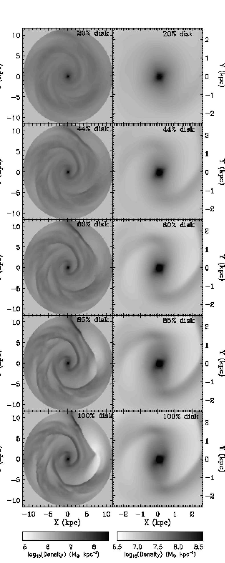
Figure 17: Grey scaled maps of the log of the density from simulations with the beam scheme on a 201 $\times$ 201 grid, with 60 per cent disk fraction, $R_{\rm c}=$7.58 kpc, $c_{\rm s}=10$$\,{\rm{\ }km{\ }s^{-1}}$ and with different disk fractions. The entire simulated region is shown in the left column and the inner 2.6 kpc² region is shown in the right column.

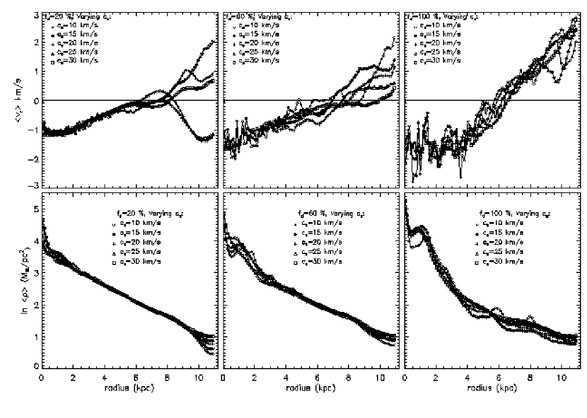
Figure 18: Plots of the density averaged radial velocity (top row) and corresponding natural logarithm of the average density (bottom row) for simulations on a 201 $\times$ 201 grid, with 20, 60 and 100 per cent disk fraction, $R_{\rm c}=$7.58 kpc, and $c_{\rm s}$ ranging from $10$$\,{\rm{\ }km{\ }s^{-1}}$ to $30$$\,{\rm{\ }km{\ }s^{-1}}$ .

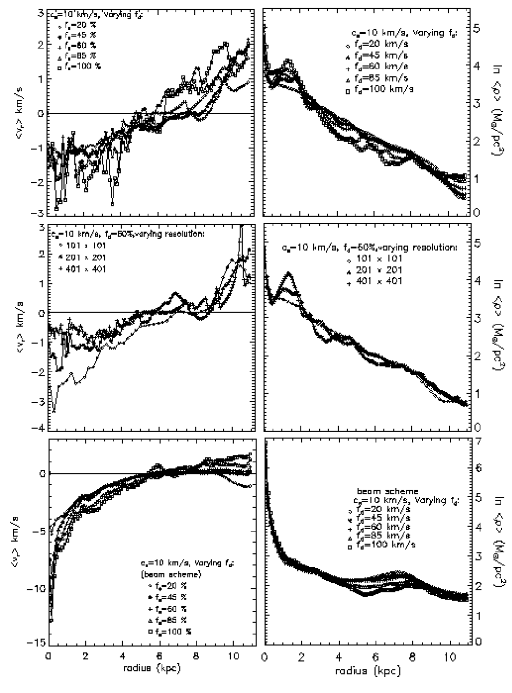
Figure 19: Plots of the mass–averaged radial velocity (left column) and corresponding natural logarithm of the average density (right column) for simulations on a 201 $\times$ 201 grid with $R_{\rm c}=$ 7.58 kpc and $c_{\rm s}=10$$\,{\rm{\ }km{\ }s^{-1}}$ . Top and bottom rows show results from simulations with disk fraction ranging from 20 per cent to 100 per cent performed with the BGK and beam scheme respectively. Middle row shows results from the BGK scheme for the 60 per cent disk case, with different grid resolutions.

4 Mass Inflow

Another way to quantify the influence of the different simulation parameters is to consider the mass inflow rates. As pointed out by Athanassoula (1992), a good indicator of the mean inflow rate is the mass-averaged radial velocity, $<v_{r}>$. Hence we compute it (fig. 18, top row; fig. 19, left column) as a function of radius for different simulations. We also plot the average densities, $<\rho>$, (fig. 18, bottom row; fig. 19, right column) so as to illustrate the net effect of the radial inflow velocity on the gas mass distribution.

Fig. 18 shows that changing the gas sound speed affects the simulations with a high disk fraction more than the simulations with a low disk fraction. More specifically, the scatter about the average radial velocity is $\approx$ 1 $\,{\rm{\ }km{\ }s^{-1}}$ for the 100 per cent disk case as opposed to $\approx$ 0.1 $\,{\rm{\ }km{\ }s^{-1}}$ for the 20 per cent disk case. The figure also shows that the maximum of $<v_{r}>$ varies from $\approx$ –1 $\,{\rm{\ }km{\ }s^{-1}}$ for the 20 per cent disk case to $\approx$ –2 $\,{\rm{\ }km{\ }s^{-1}}$ for the 100 per cent disk case. The larger $|<v_{r}>|$ for the higher disk fraction cases can be explained by the fact that increasing the disk fraction increases the strength of the spiral shocks. This in turn increases the amount of dissipation and hence angular momentum loss that the gas suffers as it slams into the shocks during its rotation about the galactic center

Fig. 18 also shows that the shape of the $<v_{r}>$ profile changes with increasing disk fraction. More specifically for the 100 per cent disk simulations the region of the disk where $|<v_{r}>|$ is maximum extends from the center to $\approx$ 3.5 kpc. As a consequence of this high inflow up to large distances the average scale length of the density distribution for the region interior to $\approx$ 3.5 kpc is much smaller than the initial gas radial scale length. In contrast, for the 20 per cent disk fraction case only the region contained within the inner 2 kpc of the disk departs in shape from the initial condition.

In addition to sensitivity to disk fraction and sound speed, the mass inflow rates, as pointed out by Prendergast (1983), are incredibly sensitive to code and grid spacing. To explore this issue, we measured $<v_{r}>$ and $<\rho>$ for simulations with different grid resolutions and also for a set of simulations done with a different code. As a worst case scenario for a diffusive grid code we took the beam scheme (Sanders and Prendergast 1974) which was used extensively in the earliest galactic disk simulations (Huntley 1978, Sanders & Tubbs 1980, Duval & Athanassoula 1983 ). Like BGK, the beam scheme is a gas-kinetic hydrocode, i.e. fluxes are computed by taking moments of a velocity distribution function, $f$. Both schemes arbitrarily choose $f$ at the beginning of each updating time-step but the beam scheme evolves it through the collisionless Boltzmann equation whereas the BGK scheme solves for the time evolution of $f$ throughout an updating time-step using the BGK equation which is a model of the collisional Boltzmann equation. By assuming instantaneous relaxation of $f$ to a Maxwellian velocity distribution at the beginning of the updating time-step, the beam scheme endows the gas with a mean collision time equivalent to the updating time-step. In the BGK scheme, on the other hand, collisions are active throughout the updating time-step and for hydrodynamical applications the BGK scheme demands that the collision time be much smaller than the updating time-step. Since dissipation parameters are proportional to the collision time, $\tau$, e.g. the dynamical viscosity $\eta=\tau$ p , we easily see that an overestimation of the collision time will lead to a very diffusive scheme. Indeed, fig. 19 illustrates that $<v_{r}>$ is about an order of magnitude larger with the beam scheme than it is with BGK and that the effect is worse in the center of the disk where a plot of $<\rho>$ shows that simulations with different disk fractions are indistinguishable. Figure 19 also shows that even with a BGK simulation on a 101 $\times$ 101 grid one still does better than beam by about a factor of 5 in the radial inflow velocities in the inner regions of the disk.

A look at the morphology of the disk for simulations performed with the beam scheme, (figure 17) confirms that the inner region of the disk computed with beam is essentially insensitive to disk fraction. The morphological changes that accompany a change in disk fraction (Fig. 8) are absent. Interestingly however, figures 19 and 17 show that even with this incredibly diffusive scheme, one can still distinguish between simulations run with different disk fractions in the outer regions of the disk where a spiral perturbation is present.

5 Discussion

Figure 20: $\chi^{2}$ comparison between simulations and observations for the set of simulations explored in this paper. All points, with the exception of the large solid points (beam scheme), are from simulations with the BGK scheme. The asterices denote simulations performed on a 201 $\times$ 201 grid, with $c_{\rm s}=10$$\,{\rm{\ }km{\ }s^{-1}}$ and $R_{\rm c}=7.58$ kpc. Open triangles indicate simulations at different resolution, and open diamonds indicate $\chi^{2}$ results from simulations at different sound speeds.

Figure 21: Plot of the average deviation of the velocity from axisymmetry for both the observations (open squares) and the simulations (asterices, filled circles, open triangles, open diamonds). The symbols for the simulations have the same meaning as the symbols in figure 20. An axisymmetric model was fit to the observation, and then this model fit was subtracted from both the observation, and the simulation. Due to differences in the axisymmetric model fit for the different disk fractions, there is a small variation in the average wiggle amplitude for the measurements.

In order to quantify what has been described in Sections 3 and 4 we perform an overall comparison between the observed and simulated kinematics. We use two approaches. First we perform a global least squares analysis (figure 20) taking into account the location and amplitudes of individual wiggles. Secondly, we compute the average wiggle amplitude (figure 21), neglecting information about the wiggle positions. The comparison was performed on a reduced data set with the very inner disk region removed. Furthermore, a treatment has been applied to the observed kinematics in order to exclude shocks that are missing from all simulations. These shocks probably originate from non-gravitational effects (see Kranz 2002, §4.3.2.1).

Figure 20 corresponds to figure 9 in Paper I (except that it uses the reduced data set described above) and measures the match in both wiggle position and amplitude between the observations and simulations. Our BGK simulations with fiducial values for the grid resolution, gas sound speed, and pattern speed are plotted with asterices. As argued in Paper I, a maximal disk mass fraction can be ruled out for NGC 4254 on the basis of this plot. Now we can look at how strongly the locations of the points in figure 20 depend on the chosen parameters for the simulations. Gradually increasing the gas sound speed (temperature) to an unphysical 30 $\,{\rm{\ }km{\ }s^{-1}}$ (90.000 K) smoothes out the wiggles in the simulations. As a result, a higher gas sound speed cancels out any change in the disk mass fraction (diamonds), so that for $c_{\rm s}=30$ $\,{\rm{\ }km{\ }s^{-1}}$ the simulated gas velocity field is almost independent of $f_{\rm d}$. However, for smaller variations ($\pm$5-10$\,{\rm{\ }km{\ }s^{-1}}$ ) of the gas sound speed relative to our fiducial value of 10 $\,{\rm{\ }km{\ }s^{-1}}$ , the effect on the least squares analysis is weak. As for the effect of the grid resolution, we studied it for the case of $f_{\rm d}=60$ per cent (triangles in figure 20). The features resulting from the simulation on the 100 $\times$ 100 grid are smoother with respect to the fiducial model, thus yielding a slightly worse agreement with the observed kinematics. On the other hand, the high resolution simulation (400 $\times$ 400 grid) yields an even worse agreement with the observations. This can be understood by studying figures 7 and 9 which show that even though the amplitude and in many cases the peak positions of the wiggles on the 201 $\times$ 201 grid have nearly converged to their values on the 401 $\times$ 401 grid, the shocks on the higher resolution grid have a different profile. They tend to be sharper and to have higher density and velocity contrast so that a measurement of the spatial overlap of the wiggles with observations finds significant discrepancies between the two models. Furthermore in comparison with the (lower resolution) observed gas kinematics the wiggles on the 401 $\times$ 401 grid exhibit larger average deviations from the data points, resulting in a worse overall $\chi^{2}/$N value. Accordingly, we argue that simulations should be performed on a grid with a cell size comparable to the spatial resolution of the observational data that they will be compared to. Alternatively one can smooth high-resolution simulations to match the spatial resolution of the observations. Finally, to explore the $\chi^{2}/$N values resulting from a different and more diffusive hydrocode, we plotted results from the beam scheme (filled circles) for simulations with fiducial values for the grid resolution, gas sound speed, and pattern speed. Figure 20 shows that the beam scheme seems to work relatively well for most of the disk regions. It should be noted however that the central region of the disk, where the beam scheme is the least successful, was excluded from the comparison.

Naively reading figure 20, we would conclude that the 45 per cent disk model is the best match to the observations. However, in light of section 3 which illustrated the unlikelihood of simple simulations exactly matching every wiggle in the observations, we make the following remarks on the $\chi^{2}$ analysis. If for a simulation performed with a given $f_{\rm d}$ there is a large amplitude wiggle which is slightly spatially shifted from the wiggle in the observation, it will give a large deviation in the $\chi^{2}$ plot. As a result, the simulation may be discarded as one which gives a poor match to the observation when in fact it could be that the simulation parameters were reasonable but not precise enough. For example, the physical sound speed at a wiggle location could have been very different from the simulation sound speed, or the pattern speed which has the greatest influence on the positions of the wiggles, is not as constant as modeled. On the contrary, the simulations with smaller wiggles, caused either by low disk fraction, high sound speed, low resolution, or a very diffusive scheme, have the advantage that even if the peaks mismatch, they are small in the simulation so they do not carry as much weight in the calculation of the $\chi^{2}$ deviations. Hence these simulations might give better $\chi^{2}$ matches. This suggests that the $\chi^{2}$ analysis favors low $f_{\rm d}$ models. This conclusion is not completely straightforward because it is not true that all processes that weaken wiggles improve the $\chi^{2}$ fit. For example, increasing the sound speed from 10 to 30 km/s for the 20% and 60% disk fraction models worsens the $\chi^{2}$. However the robust trend that emerges from our analysis is that changing the various modeling parameters for the higher $f_{\rm d}$ disks causes larger variations in the $\chi^{2}$ than changing the same parameters for the lower $f_{\rm d}$ models. In other words, getting the parameters “right” for the high $f_{\rm d}$ models is more crucial, than getting them “right” for the low $f_{\rm d}$ models. In that sense, the $\chi^{2}$ analysis favors the low $f_{\rm d}$ models. Given all the uncertainties in the modelling, variations of the $\chi^{2}$ which are smaller than 10 or 20 per cent should not be taken too seriously. Thus according to figure 20, the range for $f_{\rm d}$ lies between 0.2 and 0.85 but it is very difficult to distinguish models within this bracket. Unfortunately this range of values for $f_{\rm d}$ is very large since it allows for sub-maximal as well as marginally maximal disks.

On the other hand, figure 21 only contains information about wiggle amplitudes. These are obtained by subtracting an axisymmetric velocity field (a slowly varying function of $f_{\rm d}$, which explains the different wiggle amplitudes for the measured data points) from both the simulation velocities and the observational velocities. Figure 21 corresponds to figure 8 in Paper I where the latter displays only results from the fiducial simulations. For a fixed sound speed, the average wiggle amplitude scales almost linearly with the disk mass fraction. As mentioned earlier, for a larger disk mass fraction, an increase of the gas sound speed smears out the wiggles thus decreasing their average amplitude. Lowering the grid resolution (100 $\times$ 100) has the same effect, whereas increasing it (400 $\times$ 400) hardly makes any difference. This is consistent with what we see in the $\chi^{2}$ plot (figure 20): the amplitudes of the wiggles in the 200 $\times$ 200 simulation are almost converged to their values on the 400 $\times$ 400 grid (see also figures 7 and 9) thereby giving good agreement between the two different resolution simulations in figure 21. As in figure 20, the beam scheme seems to work as well as the BGK scheme for the outer disk. Neglecting error bars on the measurements, figure 21 favors a $\sim$ 70 per cent disk model. However, assuming an error bar of 2 km/s on the average wiggle amplitude, the permitted range for $f_{\rm d}$ according to figure 21 lies between 0.5 to 0.85. Taking the region of overlap of our two methods, we find $f_{\rm d}$ between 0.5 and 0.85. Even though both methods largely overlap in their predicted $f_{\rm d}$ values, we argued that the $\chi^{2}$ criterion is not as well suited in excluding low $f_{\rm d}$ values. Therefore for a sample of galaxies, the second criterion is slightly better, since the associate errors are random, while the errors of the $\chi^{2}$ will always weigh in favor of small $f_{d}$ values.

Following an exploration of the simulation parameter space in this paper, we understand why these global measurements do not give extremely accurate measurements of the disk fraction. However, a robust conclusion of figures 20 and 21 is that hydrodynamical simulations rule out a maximal disk model for NGC 4254, in agreement with our conclusions in Paper I and strongly suggest a value of the disk fraction in the range 50 – 85 per cent. Even when we make the gas in the disk (unreasonably) hot or when we use a very diffusive scheme, the maximal disk solution is never the best match to the observations. We conclude that the fiducial model used in Paper I is indeed close to the best if not the best estimate and that considering the simplified physics used in this analysis, our method puts surprisingly tight constraints on the amount of dark matter present in high surface brightness galaxies.

6 Conclusions

We have demonstrated that despite simplifications in modelling gas flows, hydrodynamical simulations can still put strong constraints on the dark matter fraction of spiral galaxies. Our main conclusions are:

• For the purposes of breaking the disk-halo degeneracy, modeling gas flow across massive spiral arms may be preferable to modeling the flow in the inner regions of strongly barred galaxies, because gas flow in the inner region depends more critically on the assumed sound speed of the ISM (see for example fig. 14) and suffers more from numerical viscosity (fig. 19).

• From the modelling parameters we considered, the pattern speed is by far the most important parameter for determining the gas morphology. This makes constraints on the pattern speed through comparison to the observed spiral morphology convincing.

• A detailed comparison between simulated and observed velocity fields is challenging because of the dependence of the gas flow on many physical and numerical parameters. Nevertheless, with a reasonable, physically motivated choice for the gas sound speed, a grid resolution which is comparable to the resolution of the observations, and a high-resolution hydrocode such as BGK, one can get a good estimate of the pattern speed of the gravitational potential. Then, the baryonic disk fraction remains as the primary parameter determining the flow. While the technique discussed in this paper cannot yield an exact number for the dark matter fraction in a spiral galaxy, it can constrain it, conclusively ruling out certain values for $f_{\rm d}$.

References

- [] Athanassoula, E., 1992, MNRAS, 259, 345
- [] Berman, R. H., Pollard, D. J., & Hockney, R. W., 1979, A&A, 78, 133
- [] Bertin, G., & Lin, C. C., 1996, ’Spiral Structure in Galaxies’, (Cambridge: MIT Press)
- [] Cepa, J., & Beckman, J. E., 1990, ApJ, 349, 497
- [] Colina, L., & Wada, K., 2000, ApJ, 529, 845
- [] Combes, F., & Gerin, M., 1985, A&A, 150, 327
- [] Cowie, L. L., 1980, ApJ, 236, 868
- [] Duval. M. F., & Athanassoula, E., 1983, A&A, 121, 297
- [] England, M. N., 1989, ApJ, 344, 669
- [] Englmaier, P., & Gerhard, O., 1997, MNRAS, 287, 57
- [] Garcia-Burillo, S., Combes, F., & Gerin, M., 1993, A&A, 274, 148
- [] Garcia-Burillo, S., Sempere, M. J., & Combes, F., 1994, A&A, 287, 419
- [] Goldreich, P., & Lynden-Bell, D., 1965, MNRAS, 175, 1
- [] Hunter, J. H. Jr., England, M. N., Gottesman, S. T., Ball, R., & Huntley, J. M., 1988, ApJ, 324, 721
- [] Huntley, J. M., 1978, ApJ, 225, L101
- [] Huntley, J. M., Sanders, R. H., & Roberts, W. W. Jr., 1978, ApJ, 221, 521
- [] Knapen, J. H., Beckman, J. E., Cepa, J., van der Hulst, T., & Rand, R. J., 1992, ApJ, 385, L37
- [] Knapen, J. H., Beckman, J. E., Cepa, J., & Nakai, N., 1996, A&A, 308, 27
- [] Kranz, T., 2002, PhD Thesis, University of Heidelberg. http://www.ub.uni-heidelberg.de/archiv/2214
- [] Kranz, T., Slyz, A., & Rix, H.-W., 2001, ApJ, 562, 164 (Paper I)
- [] Kranz, T., Slyz, A., & Rix, H.-W., 2003, ApJ, 586, 143
- [] Lindblad, P. A. B., Lindblad, P. O., & Athanassoula, E., 1996, A&A, 313, 65
- [] Lindblad, P. A. B. & Kristen, H., 1996, A&A, 313, 733
- [] Mulder, P. S., & Combes, F., 1996, A&A, 313, 723
- [] Patsis, P. A., & Athanassoula, E., 2000, A&A, 358, 45
- [] Prendergast, K. H., 1983, in Proc. IAU Symp. 100,’Internal kinematics and dynamics of galaxies’, Reidel, Dordrecht, ed. Athanassoula, E., p. 215
- [] Prendergast, K. H., & Xu, K., 1993, J. Comput. Phys., 109, 53
- [] Roberts W. W., 1969, ApJ, 158, 123
- [] Sanders, R. H., & Huntley, J. M., 1976, ApJ, 209, 53
- [] Sanders, R. H., & Prendergast, K. H., 1974, ApJ, 188, 489
- [] Sanders, R. H., & Tubbs, A. D., 1980, ApJ, 235, 803
- [] Schwarzkopf, U., & Dettmar, R.-J., 2000, A&A, 361, 451
- [] Sellwood, J. A., 2000, Ap&SS, 272, 31
- [] Sellwood, J. A., & Carlberg, R. G., 1984, ApJ, 282, 61
- [] Sempere, M. J., Combes, F., & Casoli, F., 1995, A&A, 299, 371
- [] Sempere, M. J., Garcia-Burillo, S., Combes, F., & Knapen, J. H., 1995, A&A, 296, 45
- [] Sempere, M. J., & Rozas, M., 1997, A&A, 317, 405
- [] Shu, F. H., Milione, V., & Roberts, W. W., 1973, ApJ, 183, 819
- [] Slyz, A., Devriendt, J., Silk, J., & Burkert, A., 2002, MNRAS, 333, 894
- [] Slyz, A., & Prendergast, K. H., 1999, A&AS, 139, 199
- [] Slyz, A., Devriendt, J., Bryan, G., & Silk, J., 2003, in preparation
- [] Sorensen, S.-A., & Matsuda, T., 1982, MNRAS, 198, 865
- [] Toomre, A., 1981, in ’Structure and Evolution of Normal Galaxies’, eds. S. M. Fall & D. Lynden-Bell (Cambridge: Cambridge University Press) p. 111
- [] Wada, K., & Koda, J., 2001, PASJ, 53, 1163
- [] Weiner, B. J., Sellwood, J. A., & Williams, T. B., 2001, ApJ, 546, 931
- [] Woodward, P. R., 1975, ApJ, 195, 61
- [] Xu, K., 1998, Gas-Kinetic Schemes for Unsteady Compressible Flow Simulations, VKI report 1998-03 von Karmann Institute Lecture Series
- [] Xu, K., & Prendergast K. H., 1994, J. Comput. Phys., 114, 9