On the 3D dynamics and morphology of inner rings

Abstract

We argue that inner rings in barred spiral galaxies are associated with specific 2D and 3D families of periodic orbits located just beyond the end of the bar. These are families located between the inner radial ultraharmonic 4:1 resonance and corotation. They are found in the upper part of a type-2 gap of the x1 characteristic, and can account for the observed ring morphologies without any help from families of the x1-tree. Due to the evolution of the stability of all these families, the ring shapes that are favored are mainly ovals, as well as polygons with ‘corners’ on the minor axis, on the sides of the bar. On the other hand pentagonal rings, or rings of the NGC 7020 type hexagon, should be less probable. The orbits that make the rings belong in their vast majority to 3D families of periodic orbits and orbits trapped around them.

1 Introduction

Rings are often observed in barred galaxies and can be spectacular structures. They come in three kinds: nuclear rings, near the nucleus of the galaxy, inner rings, surrounding the bar, and outer rings, of a considerably larger diameter. In this paper we focus our attention to the study of the inner rings. Buta (1995, hereafter B95) has made a statistical study of 3692 ring galaxies in the southern hemisphere, as well as more in depth studies of specific objects (e.g. Buta et al. 2001, 1999; Buta & Purcell 1998; Buta, Purcell & Crocker 1996). He found that inner rings are a frequently encountered feature of barred galaxies. Their mean axial ratio is $0.84\pm 0.10$, elongated along the bar major axis. This ratio, however, varies from one galactic type to another as well as among different ring morphologies (see Table VII in Buta & Combes, 1996). In some cases of typical inner rings the axis ratio can be as low as 0.63 (NGC 6782) or even 0.49 (A0106.7-3733) (Buta, 1986). B95 mentions a dozen galaxies for which there could be an intrinsic misalignment between the bar and the inner ring. Because of projection effects, however, spectroscopic measurements are necessary in order to confirm this misalignment. In the vast majority of cases the inner ring encircles the bar and touches its extremities. There are, however, cases where the bar underfills what appears to be an inner ring. Buta (1986) mentions 30 such cases in his sample of 1200 objects. Two typical examples are also given by B95, namely NGC 7098 and NGC 3450.

The link between rings and resonances has been made already in the ’70s (e.g. Schommer & Sullivan, 1976). It took, however, the advent of test particle hydrodynamic simulations in the ’80s to establish it fully. In particular, Schwarz (1981, 1984a) followed the response of gas, modeled by sticky particles, to a bar forcing. He found that ring structures can form, and that, as in real galaxies, they can be classified into outer, inner and nuclear. Schwarz linked the outer rings to the outer Lindblad resonance (OLR), the inner ones to the inner 4:1 resonance or inner ultraharmonic resonance (iUHR), and the nuclear ones to the inner Lindblad resonance (ILR). The first statistical arguments came from Athanassoula et al. (1982) who, using the sample of de Vaucouleurs & Buta (1980), showed that the ratios of inner to outer ring sizes is compatible with the outer ring being at the OLR and the inner one at corotation, or at the iUHR. This statistics has been since repeated (B95), using much better observational samples, but the result did not change.

Rings form by gas accumulation at resonances (e.g. Buta, 1999, and references therein), and this explains their predominance on images of galaxies which show best the sites of population I objects. It is, however, now clear (Athanassoula, 1992b) that the gas response is determined to a large degree by the periodic orbits in the underlying gravitational potential. For this reason, understanding the orbital dynamics of rings is essential not only for understanding their morphology per se, but also for understanding properties related to the gas component, e.g. star formation.

One of the main uses of orbital structure studies is that they provide information on the orbits that are the backbone of the various galactic structures, and thus on their morphologies. Studying the orbital structure in an appropriate Hamiltonian system we get the periodic orbits that could be responsible for the appearance of morphological features of real galaxies. We are thus interested only in stable periodic orbits, since they trap around them the regular orbits of the system. While in 2D bar models the backbone of the bar is a single family, namely the family x1 (Contopoulos, 1983), in 3D models the orbits supporting the bar are related to a whole tree of families of periodic orbits, which we called ‘x1-tree’ (Skokos et al., 2002a). Under the assumption that bars are fast, their end should be close and within corotation (Contopoulos, 1980). Due to the fact that inner rings surround the bar, one intuitively links them to stable orbits not belonging to the x1-tree, but occupying the area just beyond the bar in the real space.

Although an association of a resonance location to an inner ring can be easily done in a first approximation, there is so far no detailed study relating the various observed morphologies of inner rings to the orbital dynamics at their region. As Buta remarks “…rings include information on … the properties of periodic orbits”(Buta, 2002). This information has not been registered until now, especially for 3D barred models, and this is exactly what gave us the motivation for the present paper.

Inner rings can be either smooth, in which case we refer to them with the generic name of ‘oval’, or they can have characteristic ‘angles’, or ‘kinks’, or ‘corners’ in their outline. These can be more or less strong and, depending on their strength, may give the ring a polygonal, rather than oval, geometry. They occur at characteristic locations along the ring. Thus such ‘corners’, or ‘density enhancements’ often occur near the bar major axis, giving the ring a ‘lemon-like’ outline. In other cases, we observe that the ring is squeezed along the major axis of the bar, so that the tips of the ‘lemon’ structure vanish, the ring becomes rather polygonal-like with sides roughly parallel to the bar’s minor axis at its apocentra, and ‘corners’ close to the minor axis. Typical examples are UGC 12646 (e.g Buta & Combes, 1996, – Fig. 17), IC 4290 (see the distribution of the HII regions in Buta et al., 1998, – Fig. 8), NGC 3351 (e.g. Sandage & Bedke, 1994, panels 168, 170). In such cases it is reasonable to speak roughly about a hexagon with two sides parallel to the minor axis of the bar. The above mentioned objects (UGC 12646, IC 4290 and NGC 3351) are typical examples. Nevertheless, in most cases all these features characterize only parts of the rings and perfect symmetry, e.g. with respect to the bar major axis, is not always observed.

Despite the complexity of the observed structures of the inner rings, and the fact that they are located outside the bar, they have been in general vaguely associated with orbits at the inner 4:1 resonance (Schwarz, 1984b; Buta, 1999, 2002). Schwarz (1984b) had already realized the presence of squeezed ovals with corners. He was, however, able to reproduce them only in the case of weak bars, or by invoking a lens-like component (Schwarz, 1985). Buta (2002, – Fig.3) invokes combinations of diamond- with barrel-like orbits to explain ring morphology. In particular barrel-like orbits have been considered necessary in order to provide cloud–cloud collisions on the sides of the bars (the regions where the cloud–cloud collisions happen are indicated with “C” in Schwarz, 1984b). These orbits help in the formation of rings which have a hexagonal rather than diamond-like geometry and have two of the sides more or less parallel to the minor axis of the bar.

Note that neither every diamond-like, nor all hexagonal orbits are necessarily related with inner rings. E.g. the planar diamond-like x1 orbits in Fig. 62 in Buta & Combes (1996), taken from Contopoulos & Grosbøl (1989), are far away from the end of the bar, which is close to corotation. We also note that hexagonal rings with cusps on the major axis of the bar, and thus with two sides parallel to the major axis of the bar, are rare. There is only a notable example of this morphology, namely NGC 7020, studied by Buta (1990).

In the present paper we study the orbital behavior at the region where the appearance of inner rings is favored. We do this in the case of 3D Ferrers bars. Studying the energy width over which the various families of periodic orbits exist, their morphology, and mainly their stability, we identify the orbital behavior in four archetypical morphologies of inner rings. In section 2 we present these structures in the cases of four galaxies. In section 3 we give a brief description of the model we use for our orbital calculations, while the families which build the rings are described in section 4. Finally we discuss our results in section 5 and enumerate our conclusions in section 6.

2 Rings morphology

Let us first introduce four inner ring morphologies. Two of them are typical ovals and the two other are exceptional cases of inner rings. Although the images shown in Fig. 1 are not of high resolution, they are nevertheless able to demonstrate the features we refer to. Most inner rings are oval, sometimes with a somewhat lemon shape because of density enhancements at the bar major axis. We illustrate this latter type in Fig. 1a with an image of NGC 6782. The isophotes peak on the major axis, indicated with arrows on the second outermost isophote, giving to the ring a cuspy or pointed oval morphology. There are no “corners” close to the minor axis of the bar, which would have given to the ring a diamond shape. In Fig. 1b we show IC 4290 which has an oval ring with characteristic breaks or corners. These are indicated with arrows on the overplotted isophotes. The outermost isophote is again oval-shaped and even slightly pointed close to the major axis. The oval, however, is not smooth and forms, or gives the impression of, angles. One can also discern a structure in the form of an “T$\perp$” with the vertical part of the symbol being the bar. The two other rings given in Fig. 1 are exceptional cases. The ring in Fig. 1c has an almost pentagonal geometry. It is observed in an image of NGC 3367. It can be described as a pseudo-ring, since the ring appears to be made of segments of spiral arms. Finally in Fig. 1d we give a deprojected image of NGC 7020 (Buta, 1990), which has a type of hexagonal ring with cusps on the major axis of the bar and two sides parallel to it. The “corners” are indicated with arrows. Of course the geometrical shapes we use above are idealized and represent the complicated morphology of inner rings only schematically. They are, nevertheless, most useful as guiding lines, in the same way as perfect ellipsoids are useful for describing bars.

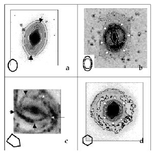
Figure 1: Examples of the four ring morphologies discussed in the paper. (a) The oval with cusps on the major axis (NGC 6782), (b) a typical oval-polygonal ring with sides parallel to the minor axis of the bar close to the ends of the bar (IC 4290), (c) a pentagonal ring in NGC 3367 and (d) the hexagonal ring with cusps on the major axis (NGC 7020). At the bottom left corner of each panel there is a sketch indicating schematically the corresponding morphology.

3 Model

To calculate the 3D ring orbits we use the fiducial case of the model described in detail in (2002a). It consists of a Miyamoto disc, a Plummer bulge and a Ferrers bar. The potential of the Miyamoto disc (Miyamoto & Nagai, 1975) is given by the formula:

$$\Phi_{D}=-\frac{GM_{D}}{\sqrt{x^{2}+y^{2}+(A+\sqrt{B^{2}+z^{2}})^{2}}}.$$ (1)

$M_{D}$ represents the total mass of the disc, $G$ is the gravitational constant, and $A$ and $B$ are scalelengths such that the ratio $B/A$ gives a measure of the flatness of the model.

The bulge is a Plummer sphere, i.e. its potential is given by:

$$\Phi_{S}=-\frac{GM_{S}}{\sqrt{x^{2}+y^{2}+z^{2}+\epsilon_{s}^{2}}},$$ (2)

where $\epsilon_{s}$ is the bulge scale length and $M_{S}$ is its total mass.

Finally, the bar is a triaxial Ferrers bar with density $\rho(x)$:

$$\rho(m)=\left\{\begin{array}[]{lcc}\displaystyle{\frac{105M_{B}}{32\pi abc}(1-m^{2})^{2}}&{\mbox{f}or}&m\leq 1\\ &&\\ \displaystyle{0}&{\mbox{f}or}&m>1\end{array}\right.,$$ (3)

where

$$m^{2}=\frac{y^{2}}{a^{2}}+\frac{x^{2}}{b^{2}}+\frac{z^{2}}{c^{2}}\,\,,\,\,\,a>b>c.$$ (4)

In the above $a$, $b$, $c$ are the principal semi-axes, and $M_{B}$ is the mass of the bar component. The corresponding potential $\Phi_{B}$ and the forces are given in Pfenniger (1984) in a closed form, well suited for numerical treatment. For the Miyamoto disc we use A=3 and B=1, and for the axes of the Ferrers bar we set a:b:c = 6:1.5:0.6. The masses of the three components satisfy $G(M_{D}+M_{S}+M_{B})=1$. We have $GM_{D}=0.82$, $GM_{S}=0.08$, $GM_{B}=0.10$ and $\epsilon_{s}=0.4$.

The length unit is taken as 1 kpc, the time unit as 1 Myr and the mass unit as $2\times 10^{11}M_{\odot}$. The bar rotates with a pattern speed $\Omega_{b}$=0.054 around the $z$-axis, which corresponds to 54 km sec^-1 kpc^-1, and places corotation at 6.13 kpc.

4 Orbits

The Hamiltonian governing the motion of a test-particle in our system can be written in the form:

$$H=\frac{1}{2}(p_{x}^{2}+p_{y}^{2}+p_{z}^{2})+V(x,y,z)-\Omega_{b}(xp_{y}-yp_{x}),$$ (5)

where $p_{x},~{}p_{y},$ and $p_{z}$ are the canonically conjugate momenta of $x$, $y$ and $z$ respectively and $V(x,y,z)$ is the total potential of the combined three components of the model: disc, bar and bulge. We will hereafter denote the numerical value of the Hamiltonian by $E_{j}$ and refer to it as the Jacobi constant or, more loosely, as the ‘energy’.

A periodic orbit in a 3D Hamiltonian system can be either stable ($S$) or exhibit various types of instability. It can be simple unstable ($U$), double unstable ($D$) or complex unstable ($\Delta$) (for definitions see Contopoulos, 2002, chapter 2.11). The method used for finding periodic orbits and their stability is described in detail in (2002a) and in references therein. Periodic orbits are grouped in families, along which the energy $E_{j}$ changes and the stability of the orbits may also change. The S $\rightarrow$ U transitions of periodic orbits are of special importance for the dynamics of a system, since in this case a new stable family is generated by bifurcation. A useful diagram for presenting the various periodic orbits of the system is the ‘characteristic’ diagram (Contopoulos, 2002, section 2.4.3). It gives the $x$ coordinate of the initial conditions of the periodic orbits of a family as a function of their Jacobi constant $E_{j}$. In the case of orbits lying on the equatorial plane ($z=p_{z}=0$) and starting perpendicular to the $x$ axis ($p_{x}=0$), with $y=0$ and $p_{y}>0$, we need only one initial condition, $x$, in order to specify a periodic orbit on the characteristic diagram. Thus, the initial conditions of such orbits are fully determined by a point on the characteristic diagram. Initial conditions of orbits which stay on the equatorial plane but do not start perpendicular to the $x$ axis and of orbits which do not stay on the equatorial plane are not fully defined by their $x$ coordinate. In these, more general cases, the representation on the $(E_{j},x)$ diagram is not very useful.

In our model, the highest energy orbits that support the bar can be found at the region of the radial 4:1 resonance (, 2002a; Patsis et al., 2003). Since the rings surround the bars, we first look for families of periodic orbits beyond the energy which corresponds to this resonance and we follow their stability as we approach corotation. Athanassoula (1992a) has found several families of orbits beyond the 4:1 resonance in 2D Ferrers bars (see Figs. 2 and 3 of that paper). We did not know, however, which of those could trap matter around them and support ring structures, because their stability was not studied in that paper. We address this problem here in the more general case of a 3D Ferrers bar.

4.0.1 The f-group

In all 3D Ferrers bars studied by Skokos et al. (2002a, b) the characteristic of the x1 family has $x$ values which increase with $E_{j}$ until a maximum is reached, at which point the $x$ values start decreasing. Beyond the local maximum we find the characteristics of other families, which for larger $E_{j}$ have initial $x$’s which are larger than those of x1. In other words, we have type-2 gaps (Contopoulos & Grosbøl, 1989). In 2D models of barred galaxies the family found beyond the local maximum is the family x₁(2) (Contopoulos, 2002, Fig. 3.8b in). In our 3D models the first family we find beyond the gap is a 2D 4:1 family, which we call f. Its morphology is rhomboidal as the morphologies of the corresponding families of the 2D models in Contopoulos & Grosbøl (1989) and Athanassoula (1992a). However, in the 3D model, it is accompanied by a forest of bifurcating families. We call this group of families of periodic orbits the ‘f-group’.

In Fig. 2 we give the ($E_{j},x$) characteristic of f, which is the small curve above the x1 characteristic indicated with f. The lower part of the curve, i.e. smaller $x$ for the same $E_{j}$, is composed mainly of stable f orbits. Nevertheless, instability strips do exist, but are not important. The upper part of the curve is mainly composed of unstable orbits. In the figure black segments indicate stability and grey instability. For the sake of clarity we do not include in the figure the projections of the characteristics of the 2D and 3D families bifurcating from f.

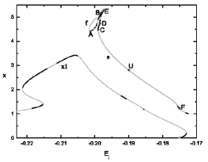
Figure 2: Characteristic diagram of families x1, f and s. We observe a typical type-2 gap at the radial 4:1 resonance region. Stable parts are indicated with black lines and unstable ones with grey lines. The capital letters A to F, as well as U, indicate the location of specific orbits which are discussed further in the text. At this diagram L_4,5 would be at $\approx$ ($-0.1955,6.0$).

The ‘mother’ planar 2D f-family starts existing at about $E_{j}\approx-0.20166$, and the morphology of its orbits is as in Fig. 3a. It remains basically stable until $E_{j}\approx-0.198$, with only small instability regions in between. With increasing energy, the morphology of the f orbits changes and becomes hexagonal (Fig. 3b). We thus have a smooth transition from a basically 4:1 to a 6:1 morphology. The two points marked “A” and “B” on the stable part of the characteristic indicate the location of the two f-orbits shown in Fig. 3a and Fig. 3b, respectively. Beyond $E_{j}\approx-0.198$ the orbital multiplicity, i.e. the number of intersections of the periodic orbit with the $x$-axis before it closes, changes. At an S$\rightarrow$U$\rightarrow$S transition close to $E_{j}\approx-0.2004$ we have two 5:1-type 2D families bifurcated from f. Namely, fr1 (Fig. 3c) at an S$\rightarrow$U transition, and fr2 (Fig. 3d) at the nearby U$\rightarrow$S transition. We note that fr1 orbits do not start perpendicular to the $x$ axis. For these and all the rest of the bifurcating families in the paper we follow the nomenclature rules introduced in (2002a). Soon after its bifurcation, however, the stable fr1 family becomes unstable, while the initially unstable fr2 becomes stable. The f orbits along the unstable part of the characteristic are diamonds with cusps on the axes (Fig. 4). These orbits are characterized by segments, which resemble straight line sides.

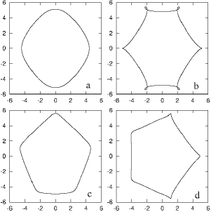
Figure 3: 2D f-orbits. In (a) and (b) we have stable f orbits located at points “A” and “B” on the f characteristic in Fig. 2. In panels (c) and (d) we give typical stable fr1 and fr2 orbits. In this and subsequent figures the bar major axis lies along the $y$-axis and the units are in kpc.

Figure 4: A 2D unstable f-orbit from the upper part of the f-characteristic (drawn with a grey line in Fig. 2).

Stable 3D families are introduced at S$\rightarrow$U transitions of family f at $E_{j}\approx-0.2016$, $-0.2002$ and $-0.1993$, and are the families fv1, fv3 and fv5, respectively. These families, together with their stable bifurcations, contribute significant stable parts to the area. The three projections of five orbits of 3D families of the f-group are given in Fig. 5. The two orbits at the top of the figure belong to family fv1, for $E_{j}=-0.201$ and $-0.181$ respectively, and show that the morphological evolution of the $(x,y)$ projection of this family follows the morphological evolution of the 2D family f. The third and fourth rows from the top give the morphology of orbits from two bifurcations of family fv1, which in turn has bifurcated from family f. They are introduced in the system as stable, but do not have large stability parts, since they become soon unstable. The fifth and the sixth orbits from the top belong to family fv3, and are given for $E_{j}=-0.200$ and $-0.193$, respectively. The morphology of their $(x,y)$ projections is again similar to the morphology of a 2D f-type family (Fig. 3a,b) of the same energy. Finally the last orbit is an example of an orbit from family fv5, close to its bifurcating point. We note that fv5 becomes complex unstable at $E_{j}=-0.19697$. At this energy it has already large deviations above and below the equatorial plane, i.e. large $\overline{|z|}$ values, and thus it would not contribute significantly to the local disc density, even if it was stable.

Figure 5: Stable 3D f-orbits. The names of the families are noted on the right side of each set of projections. The projection planes are indicated in the upper left corner of each frame.

4.0.2 The s-group

In Fig. 2 we see that, below and to the right of the characteristic of f, there is another, longer curve, roughly speaking parallel to the decreasing branch of x1. This is the characteristic of a 2D 6:1 family, which we call “s”. It exists for $E_{j}>-0.1990$. As in the case of the f-group, we have here a group of families of periodic orbits (s-group). The group includes s and several 2D and 3D families bifurcated from it. The stable part is the one with the larger $x$’s for the same energy. As in the previous case, along the stable part we have a morphological evolution of the orbits and tiny instability strips, where new families are born. We can follow the morphological evolution of the s family of orbits in Fig. 6 from (a) to (b) and to (c). They correspond to the points labeled on the characteristic of s in Fig. 2 with the capital letters “C”, “D” and “E”, respectively. Along the characteristic of s we have a smooth transition from a basically 6:1 to an 8:1 morphology. An S$\rightarrow$U transition at $E_{j}\approx-0.19876$ introduces in the system the planar stable family sr1 (Fig. 6d), which is a 7:1 type orbit. Along the long unstable part of the s characteristic, orbits are hexagonal with cusps on the major axis of the bar (Fig. 6e). Family s has another stable part at the largest $E_{j}$’s and small $x$ values (see Fig. 2). However, the morphology of the s orbits at these energies is characterized by big loops (Fig. 6f), so that they cannot be used to build rings.

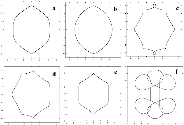
Figure 6: 2D orbits of the s-group. From (a) to (b) and then to (c) we see the evolution of the orbital morphology along the stable branch of the s characteristic as we move from “C” to “D” to “E” (Fig. 2). In (d) we observe a planar stable sr1 orbit, in (e) an unstable s orbit (point U in Fig. 2), and in (f) a stable s orbit with loops (point F in Fig. 2).

At three other S$\rightarrow$U transitions with tiny unstable parts, at $E_{j}\approx-0.19892,E_{j}\approx-0.19869$ and $E_{j}\approx-0.1984$ respectively, three stable 3D families bifurcate. From smaller to larger energies, we call them sv1, sv3 and sv5. Fig. 7 gives the morphology of these families. In Fig. 7a we observe the three projections of sv1 close to its bifurcating point. In Fig. 7b we give sv3 also close to its bifurcating point and in Fig. 7c at larger energies. Finally Fig. 7d shows sv5 just after its bifurcation from s. The morphological evolution of the face-on projections of the 3D families resembles the evolution of the stable s orbits as the energy increases. Both sv3 and sv5 families have complex unstable parts, starting from $E_{j}\approx-0.19424$ and $E_{j}\approx-0.1972$ respectively. However, as in the case of fv5, this happens at energies where $\overline{|z|}$ is large, and thus the orbits of these families at these energies are not significant for the local disc density.

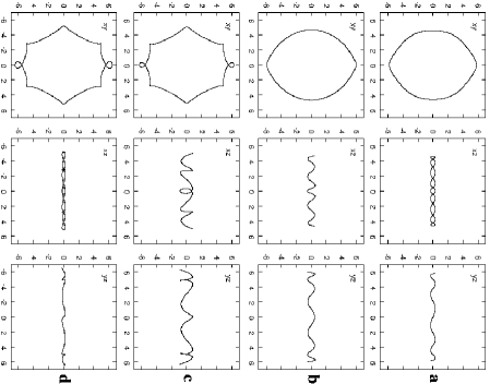
Figure 7: Stable 3D orbits of the s-group. (a) orbit from the sv1 family, (b) sv3 orbit close to the bifurcating point, (c) sv3 orbit away of the bifurcating point, (d) orbit from the sv5 family.

5 Discussion

In 3D Ferrers bars, families of periodic orbits beyond the gap at the 4:1 radial resonance, where the characteristic of the planar x1 family has a local maximum (Fig. 2), are introduced through tangent bifurcations (see Contopoulos, 2002, pg.102 for a definition). Tangent bifurcations are fundamental to the study of nonlinear systems since they are one of the most basic processes by which families of periodic orbits are created. In 2D barred potentials they correspond to the gaps at the even radial resonances (Contopoulos & Grosbøl, 1989). In such a bifurcation a pair of families of periodic orbits is created “out of nothing”. They are also referred to as saddle-node bifurcations. One of the newborn sequences of orbits is unstable (the saddle), while the other is stable (the node). A characteristic diagram of this type of bifurcations is shown schematically in Fig. 8. The characteristics of families f and s in Fig. 2 are of this type, which means that these families are not connected to the x1-tree. Furthermore, they build their own group of families, i.e. their own trees. Despite the fact that the stability is not indicated, one can see from the shape of the characteristics that in the 2D Ferrers bar model in Athanassoula (1992a) the families in the upper part of the 4:1 resonance gap are introduced via tangent bifurcations.

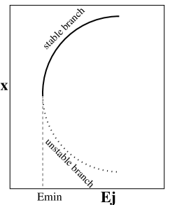
Figure 8: Schematic representation of a tangent bifurcation. The family starts existing for energies larger than $E_{min}$.

Close to the $E_{j}$ minimum at which the f and s families appear, the orbits are characterized by 4:1 and 6:1 morphologies, respectively. As we move along the stable branch towards higher values of $E_{j}$, the f orbits initially become rounder, and then for yet larger $E_{j}$, they develop cusps along the minor axis of the bar, evolving morphologically, roughly speaking, to a hexagon. Note that this hexagon has two sides parallel to the minor axis of the bar. The morphological evolution of the stable s orbits forms a similar sequence, now from a 6:1 to an 8:1 morphology, again via an ovalish shape. Note, however, that the geometrical shape of the orbit depicted in Fig. 6a changes very fast, i.e. the s orbits have this morphology only in a very tiny energy interval. It evolves to a lens-type morphology and finally to the octagonal shape we see in Fig. 6c, which develops loops along the major axis of the bar. In order to visualize a collective effect of the presence of such octagonal orbits in the system, we plot in Fig. 9 successive orbits of this type selected at equally spaced intervals in energy. This could lead to an octagonal ring or, most likely, to a hexagonal ring with additional density enhancements close to the major axis of the bar. The shapes of the rings that are favored due to the stability of the planar f and s orbits can be described in general as ovals. Hexagonal morphologies support motion parallel to the minor axis at the apocentra of the rings.

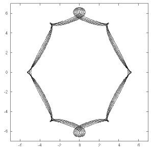
Figure 9: A set of stable, octagonal s orbits. Note that, while the outer boundary is octagonal, the inner boundary tends to a hexagonal shape.

The 2D radial bifurcations from f and s are associated with the 5:1 and 7:1 resonances, respectively. The corresponding 5:1 and 7:1 families come in pairs, with orbits symmetric with respect to the bar major axis. Thus, although they do have stable parts, they do not in general support a particular morphology if we consider both of their branches. Indeed, two 5:1 symmetric periodic orbits together represent a 10:1 morphology. In this case, non-periodic orbits trapped around them will practically contribute to the formation of a smooth ring around the bar. In cases where only one of the two branches is populated, the ring will have a mainly pentagonal or heptagonal geometry.

The existence of the 3D families is very important for the prevalence of a ring structure around the bar, because they extend the volume of the phase space occupied by stable ring-supporting orbits. Such families are introduced at the S$\rightarrow$U transitions of our model and some of their members are plotted in Figs. 5 and 7. Their vertical thickness in the z direction remains low for considerable energy intervals, at least for the orbits with face-on projections without cusps or loops (Fig. 7). This is in good agreement with observations, since inner rings have never been seen to stick out of the equatorial plane in galaxies which are observed edge-on. These new families remain practically stable for energy intervals over which their face-on projections, and the corresponding f or s ‘mother’ families support the ring. On the other hand, over the energy intervals where these families are complex unstable, their face-on projections have loops and their average height above the equatorial plane has also increased. Since they are complex unstable they are not associated with further bifurcating families (for definitions related with instabilities in 3D systems see e.g. Contopoulos, 2002). The presence of complex instability introduces chaos in the system, however at energies for which the families have members reaching large distances above and below the equatorial plane. Thus their importance for the density of the rings is already small.

The two groups of f and s families of periodic orbits include practically all relevant morphologies of orbits one can find between the radial 4:1 resonance and corotation. Although we can not exclude the existence of n:1 (n$>$8) type families, we didn’t find any such orbit remaining close to the equatorial plane. Since, furthermore, the f and s family orbits are sufficient on their own to account for the rings, we do not discuss the n:1 (n$>$8) orbits any further.

5.1 Interpretation of the ring morphologies

In this section we will show that inner ring morphologies can be built using combinations of orbits of the stable 2D and 3D families which we described in the previous sections. Let us start with the most common morphologies. There is a large number of orbital combinations allowing the formation of the types of rings illustrated in Figs. 1a and b. The morphology of the s orbits that have an outline as that shown in Fig. 6b renders well that of the most frequently encountered inner rings (Fig. 1a). This is still true if we add to them stable sv1 and sv3 orbits, as those depicted in Figs. 7a and b, respectively. In order to demonstrate this, we give in Fig. 10a the face-on profile of the weighted oval- or lemon-shaped orbits of families s for $-0.1990<E_{j}<-0.1985$, sv1 for $-0.1989<E_{j}<-0.1968$ and sv3 for $-0.1987<E_{j}<-0.1982$ and $-0.1976<E_{j}<-0.1958$ (sv3 is simple unstable for $-0.1982<E_{j}<-0.1976$). These intervals have been chosen so as to exclude all unstable orbits and all orbits with $\overline{|z|}>0.8$. We consider orbits with $\overline{|z|}>0.8$ as contributing little to the rings density. We use the same technique as in Patsis, Skokos & Athanassoula ( 2002, 2003). Namely, we first calculate the set of periodic orbits which we intend to use in order to build the profile. Then we pick points along each orbit at equal time steps. The ‘mean density’ of each orbit (see Patsis et al., 2002, – section 2.2) is considered to be a first approximation of the importance of the orbit and is used to weight it. We construct an image (normalized over its total intensity) for each calculated and weighted orbit, and then, by combining sets of such orbits, we construct the weighted profile. The selected stable orbits are equally spaced in their mean radius. The step in mean radius is the same for all families in a figure.

In Fig. 10a we observe that all orbits of the s, sv1 and sv3 families are confined inside a very narrow ring. Families sv1 and sv3 are 3D. The orbits considered here are also vertically confined to a thin layer of a few hundreds pc having in the middle the equatorial plane of the galaxy model. For this, and all subsequent similar figures, we give in Tab.1 the energy intervals from which we have taken the orbits of a family in order to construct the profile. For building the profile we used orbits from all the available energy intervals. Due to the orbital crowding inside the ring, the orbits of the three families intersect each other, and thus the corresponding gas flow will be characterized by the presence of numerous cloud collisions in the same area.

Table 1: Energy intervals for the stable orbits contributing to the weighted profiles in Fig. 10 and Fig. 12. The successive columns give the name of the family and the corresponding energy intervals in the figures: 10a, 10b, 10c, 12a and 12b.

family	10a	10b	10c	12a	12b
s	$-0.1990\rightarrow-0.1985$	$-0.1990\rightarrow-0.1985$	$-0.1990\rightarrow-0.1985$	–	$-0.1984\rightarrow-0.1972$
sv1	$-0.1989\rightarrow-0.1968$	$-0.1989\rightarrow-0.1968$	$-0.1989\rightarrow-0.1968$	–	–
sv3	$-0.1987\rightarrow-0.1982$	$-0.1987\rightarrow-0.1982$	$-0.1987\rightarrow-0.1982$	–	–
	$-0.1976\rightarrow-0.1958$	$-0.1976\rightarrow-0.1958$	$-0.1976\rightarrow-0.1958$
sv5	–	–	–	–	$-0.1984\rightarrow-0.1972$
f	–	$-0.2016\rightarrow-0.1993$	$-0.2016\rightarrow-0.1993$	$-0.1990\rightarrow-0.1978$	$-0.1990\rightarrow-0.1978$
fv1	–	$-0.2016\rightarrow-0.1974$	$-0.2016\rightarrow-0.1974$	–	–
fv3	–	$-0.2002\rightarrow-0.1967$	$-0.2002\rightarrow-0.1967$	–	–
fv5	–	–	–	$-0.1993\rightarrow-0.1969$	$-0.1993\rightarrow-0.1969$

Figure 10: Weighted profiles obtained from stable orbits of families s, sv1 and sv3 (a) and s, sv1, sv3, f, fv1 and fv3 (b). In (c) we give a blurred representation of (b) and we see clearly a polygonal structure embedded in the ring. Colour in this last frame gives the projected surface density. The orbits are chosen at the appropriate energy intervals in order to support an oval shaped ring.

If we add, on top of this, orbits trapped around f, fv1 and fv3, at the appropriate energy intervals, the morphology of the ring does not change significantly. In Fig. 10b we add stable orbits belonging to the families f for small energies ($-0.2016<E_{j}<-0.1993$), fv1 for $-0.2016<E_{j}<-0.1974$ and fv3 for $-0.2002<E_{j}<-0.1967$. Again orbits with $\overline{|z|}>0.8$ are excluded. The total energy width over which the oval-building orbits exist and specify the morphology of the inner ring is $\Delta E_{j}=0.0058$. The contribution of 2D families is over a width $\Delta E_{j}=0.0028$, while the 3D families support rings in an interval $\Delta E_{j}=0.0058$. This indicates that 3D orbits are essential in building inner rings. It is also evident that the width of the ring in the face-on view is set by the contribution of orbits belonging to the f-tree. These orbits could be the origin of broader inner rings observed in the near-infrared.

In Fig. 10c we apply a gaussian filter to the image of Fig. 10b, in order to show, in a first approximation, the shapes of secondary features which could be supported by the orbits discussed here. The colour bar below it shows the correspondence of colours and surface density on the ring. As we move to the right on the colour bar the surface density increases. Colour helps in distinguishing the main features supported by the orbits in our model. It is clear that, depending on the family which prevails, we could have the following cases: (a) If the ring consists of s, sv1 and sv3 orbits at low energies it will be an oval with a more or less strong lemon shape, i.e. a morphology similar to the one of the NGC 6782 inner ring, (b) If the families of the f-tree are dominant, they will lead to the appearance of more hexagonal-like oval structures with corners close to the minor axis (like in UGC 12646), (c) A combination of all oval-supporting families, leads to the lemon-shaped oval, together with segments parallel to the minor axis and corners close to the minor axis of the bar. This is the morphology of the inner ring of IC 4290 and is represented in most of its details in Fig. 10c.

For the rings it is crucial that their width (in the equatorial plane) is not too large and this is indeed the case in Fig. 10c. In such a blurred image the filtering simulates the effect of trapping around the relevant periodic orbits. To show that the width of the gaussian that we have adopted for the filtering is reasonable, we examined the ring structure formed by single regular orbits, trapped around the periodic orbits discussed above. We found that it is well confined on the face-on view of the model, as Fig. 11 shows. This is due to the nature of the characteristic diagram in the region under consideration, since there a small deviation in the initial conditions is sufficient to stop the orbit from being trapped around the ring-producing periodic orbits. I.e. the trapping around the periodic orbits, whenever it happens, is of rather small extent. This means that the rings composed of such orbits will have small width, in good agreement with the observations.

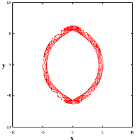
Figure 11: A single non-periodic orbit trapped around the stable s periodic orbit at $E_{j}=-0.0198176$. It is integrated for more than 20 orbital periods. It forms an oval of small width, the inner boundary of which is lemon-shaped.

In Fig. 12a we give another face-on weighted profile consisting of stable orbits of the families f at energies $-0.1990<E_{j}<-0.1978$ and fv5 at energies $-0.1993<E_{j}<-0.1969$. In Fig. 12b we add also orbits from s for $-0.1984<E_{j}<-0.1972$ and sv5 for $-0.1984<E_{j}<-0.1972$. This combination gives another type of rings, which can be described as polygonal. The orbits, as we have seen in the description of the individual families, are of 6:1 and 8:1 types. The overall polygonal morphology, in Fig. 12b, however, can be described as hexagonal. The inner ring of NGC 3351 could be explained based on these families.

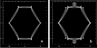
Figure 12: Weighted profiles obtained from stable orbits of families f and fv5 of the f-tree (a), and s, sv5, f, and fv5 (b). These are orbits at larger energies than the orbits of the s, f families used for the weighted profiles in Fig. 10.

The morphologies in Figs. 1c,d can also be explained with the stable orbits of the region, but only as specific cases, contrarily to the many possible combinations of orbits we can use for building the inner ring morphologies in Figs. 1a,b. A 5:1 morphology (Figs. 1c) can be explained by combination of orbits belonging to fr1 (Fig. 3c), or to fv1.1 (Fig. 5), or to both. There are, however, two problems. First, as we noted before, we can have a pentagonal symmetry when only one of the two symmetric branches of the family is populated, which presumably necessitates specific initial conditions. The second is that these families have small stability regions. Both are bifurcated as stable and become unstable for an energy close to the bifurcating point. For these two reasons pentagonal rings like in the case of NGC 3367 should be rare.

Hexagonal rings with cusps on the major axis of the bar can be formed by material trapped around periodic orbits near the energy minimum of the tangent bifurcation which brings family s in the system. Nevertheless, stable s orbits with the morphology shown in Fig. 6a exist only in a very narrow energy interval. The transition to the morphology of Fig. 6b happens very fast, while the orbit in Fig. 6e is an example from the unstable branch of the tangent bifurcation, which remains unstable for a large energy interval. Indeed, these orbits become stable only when they have developed large loops. The rarity of inner rings of the hexagonal type seen in NGC 7020 (Buta, 1990) reflects the way family s is introduced in the system through the tangent bifurcation. The stable branch of this bifurcation is associated with the formation of ovals, while the unstable one is associated with ‘NGC 7020-type’ hexagons. The morphology of the stable and the unstable orbits is very similar only very close to the energy minimum of the s characteristic. Thus, the hexagonal geometry we observe in NGC 7020 can be due only to non-periodic orbits trapped in this small fraction of the phase space. Note that the inner side of many 2D and 3D banana-like orbits trapped around the Lagrangian points L₄ and L₅, considered in pairs, can also form hexagons (see , 2002a, – Figs. 18 and 19). They can not, however, explain rings, because of their orientation. If we would consider at a given energy the two stable banana-like orbits trapped around L₄ and L₅, respectively, we build a ring elongated along the minor axis of the bar rather than around the major axis (Patsis et al., 2003, Fig.2), which is contrary to observations.

Finally we note that NGC 6782 gives also an example of diamond morphology in the bar, due to orbits with that shape, which is not related to the ring. This can be realized by inspection of the innermost isophote drawn in Fig. 1a. These isophotes may correspond to x1 diamond-shaped orbits.

6 Conclusions

We have studied the orbital structure of inner rings in static 3D Ferrers bars. The stable orbits we find belong to families which are typical for barred potentials with a type-2 gap in their characteristic at the radial 4:1 resonance. In 2D (Athanassoula, 1992a) and 3D (, 2002b) Ferrers bars this is the usual type of gap we encounter. So we expect our conclusions to be valid for a large area of the parameter space. This work is the first step in a study of ring structures encountered in time-dependent, fully self-consistent $N$-body, as well as in gaseous-response models.

The main conclusions of the present study are the following:

1. In 3D Ferrers bars, inner rings are due to orbits belonging to families in the upper part of the type-2 gap at the inner radial 4:1 resonance. They are grouped in two orbital trees, which have as mother-families the planar f and s orbits. For building the rings one cannot invoke orbits from the x1-tree or other families. The orbits that make the rings belong in their vast majority to three-dimensional families of periodic orbits.

2. The 3D bifurcating families of the two groups (fv1, fv3, fv5; sv1, sv3, sv5) play a crucial role in the morphology of the inner rings. They have large stable parts and thus they increase considerably the volume of the phase space occupied by ring-supporting orbits. The energy width over which we can find stable 3D orbits supporting the rings is larger than the corresponding interval of 2D stable families.

3. The prevailing types of inner rings are variations of oval shapes and are determined by the way the f and s families are introduced in the system, i.e. by the tangent bifurcation mechanism. The orbits on the stable branch of their characteristic, together with their stable 3D bifurcations, support ovals with a more or less strong lemon shape, or oval-polygonal rings with ‘corners’ along the minor axis of the bar. These types of inner rings represent frequently observed morphologies.

4. Pentagonal rings are rare because the families building them (fr1, fv1.1) have small stable parts and usually come in symmetric pairs. Thus, in order for these rings to appear, the symmetry must be broken and only one of the two branches be populated due to some particular formation scenario. Furthermore, considerable material should be on regular non-periodic orbits trapped around stable periodic orbits existing only in narrow energy ranges.

5. If orbits are trapped around stable s periodic orbits at the energy minimum of the s characteristic, then an NGC 7020 morphology can be reproduced. Although such a morphology is in principle possible, it should be rare, because it would necessitate that considerable amount of material be on regular orbits trapped around periodic orbits in a very narrow energy interval. Indeed the hexagonal orbits with cusps on the major axis are on the unstable branch of the tangent bifurcation.

References

- Athanassoula (1992a) Athanassoula E., 1992a, MNRAS, 259, 328
- Athanassoula (1992b) Athanassoula E., 1992b, MNRAS, 259, 345
- Athanassoula et al. (1982) Athanassoula E., Bosma A., Crézé M., Schwarz M. P., 1982, A&A, 107, 101
- Buta (1986) Buta R., 1986, ApJS, 61, 609
- Buta (1990) Buta R., 1990, ApJ, 356, 87
- Buta (1995) Buta R., 1995, ApJS, 96, 39
- Buta (1999) Buta R., 1999, Ap&SS, 269/270, 79
- Buta (2002) Buta R., 2002, in Athanassoula E., Bosma A., Mujica R., eds., ASP Conference Series, Vol. 275, Disk of Galaxies: Kinematics Dynamics and Perturbations, p. 185
- Buta & Combes (1996) Buta R., Combes F., 1996, Fund. Cos. Phys., 17, 95
- Buta & Purcell (1998) Buta R., Purcell G.B., 1998, AJ, 115, 484
- Buta et al. (1996) Buta R., Purcell G.B., Crocker D. A., 1996, AJ, 111, 983
- Buta et al. (1998) Buta R., Alpert A.J., Cobb M.L., Crocker D.A., Purcell G.B., 1998, AJ, 116, 1142
- Buta et al. (1999) Buta R., Purcell G.B., Cobb M.L., Crocker D.A., Rautiainen P., Salo H., 1999, AJ, 117, 778
- Buta et al. (2001) Buta R., Ryder S.D., Madsen G.J., Wesson K., Crocker D. A., Combes F., 2001, AJ, 121, 225
- Contopoulos (1980) Contopoulos G. 1980, A&A, 81, 198
- Contopoulos (1983) Contopoulos G. 1983, Physica D, 142
- Contopoulos (1988) Contopoulos G. 1988, A&A, 201, 44
- Contopoulos (2002) Contopoulos G., 2002, Order and Chaos in Dynamical Astronomy, Springer-Verlag Berlin Heidelberg
- Contopoulos & Grosbøl (1989) Contopoulos G., Grosbøl P., 1989, A&A Rev., 1, 261
- de Vaucouleurs & Buta (1980) De Vaucouleurs G., Buta R., 1980, AJ, 85, 637
- Miyamoto & Nagai (1975) Miyamoto M., Nagai R., 1975, PASJ, 27, 533
- Patsis et al. ( 2002) Patsis P.A., Skokos Ch., Athanassoula E. 2002, MNRAS, 337, 578
- Patsis et al. ( 2003) Patsis P.A., Skokos Ch., Athanassoula E., 2003, MNRAS, 342, 69
- Pfenniger (1984) Pfenniger D., 1984, A&A, 134, 373
- Sandage & Bedke (1994) Sandage A., Bedke J., 1994, The Carnegie Atlas of Galaxies, Vol.II., Carnegie Institute of Washington with the Flintridge Foundation, Washington D.C.
- Schommer & Sullivan (1976) Schommer R.A., Sullivan T.W., 1976, Astrophys. Lett., 17, 191
- Schwarz (1981) Schwarz M.P., 1981, ApJ, 247, 77
- Schwarz (1984a) Schwarz M.P., 1984a, MNRAS, 209, 93
- Schwarz (1984b) Schwarz M.P., 1984b, PASAu 5, 464
- Schwarz (1985) Schwarz M.P., 1985, PASAu 6, 205
- (31) Skokos Ch., Patsis P.A., Athanassoula E., 2002a, MNRAS, 333, 847
- (32) Skokos Ch., Patsis P.A., Athanassoula E., 2002b, MNRAS, 333, 861