Ni abundance in the core of the Perseus Cluster: an answer to the significance of resonant scattering

Abstract

Using an XMM-Newton observation of the Perseus cluster we show that the excess in the flux of the 7-8 keV line complex previously detected by ASCA and BeppoSAX is due to an overabundance of Nickel rather than to an anomalously high Fe He$\beta$/Fe He$\alpha$ ratio. This observational fact leads to the main result that resonant scattering, which was assumed to be responsible for the supposed anomalous Fe He$\beta$/Fe He$\alpha$ ratio, is no longer required. The absence of resonant scattering points towards the presence of significant gas motions (either turbulent or laminar) in the core of the Perseus cluster.

1 Introduction

The X-ray emission from clusters is due to a diffuse, tenuous (with typical densities of $10^{-4}-10^{-2}\,\rm{cm}^{-}3$), and hot (with typical temperatures of $10^{7}-10^{8}\,\rm{K}$) thermal plasma. Although for these ranges of density and temperature the gas is optically thin to Thomson scattering for the continuum, it can be optically thick in the resonance X-ray lines of highly ionized atoms of heavy elements (Gilfanov et al., 1987). Apart from other interesting observable effects (Sazonov et al., 2002), the major effect of resonance scattering (the absorption of a line photon followed by immediate re-emission) is to distort the surface-brightness profile of the cluster in the resonance line due to diffusion of photons from the dense core into the outer regions of the cluster. This must be taken into account when attempting to determine element abundances from X-ray spectroscopic observations of galaxy clusters. In fact only with the key assumption that the plasma is optically thin lines equivalent widths can unambiguously convert to element abundances, when fitting CCD spectra with the available plasma codes. In presence of resonant scattering the true abundances in the core of clusters are significantly underestimated because the line emission is attenuated due to photons scattered out of the line of sight. To make things worse, the most promising line for resonant scattering is the He$\alpha$ Fe emission line at 6.7 keV (Gilfanov et al., 1987; Sazonov et al., 2002) which is also one of the most prominent emission line in cluster spectra and in general drives the global abundance determination.

High sensitivity and high resolution spectrometers are needed to directly measure the spectral features of resonant scattering (as modification of the line profile or resolution of the He-like line into its constituents in order to determine directly the effects of scattering) and polarimeters, to detect the polarized scattered radiation (Costa et al., 2001; Sazonov et al., 2002). Currently the simplest method to reveal and estimate the presence of resonance scattering is to compare the fluxes of an expected optically thick line and of an optically thin one and to check if it is correctly modeled by a plasma code assuming optically thin emission. This was done in the past with ASCA and BeppoSAX for the ratio between He$\alpha$ Fe line at 6.7 keV and the He$\beta$ Fe line at 7.90 keV (which is expected to have an optical depth typically smaller than one for resonant scattering) and in particular the best data were the ones for the Perseus cluster.

Molendi et al. (1998) analyzed data collected with the MECS on board BeppoSAX and found that the ratio of the flux of the 7-8 keV line complex to the 6.7 keV line was significantly larger than predicted by optically thin plasma code and that the ratio decreases with increasing cluster radius. They noted that this effect could be explained either by resonant scattering or by a Ni overabundance, eventually favoring the former explanation. On the contrary Dupke & Arnaud (2001), according to the experimental evidence of a central enhancement of SNIa ejecta in cD clusters, favored the over-abundant Ni explanation.

These were the two hypothesis that the resolution and sensitivity of past instruments could not resolve. XMM-Newton has now for the first time the combination of resolution and effective area at high energies to give an unambiguous answer to the question. In this paper our aim is to try to solve this controversy. A complete spectral and spatial analysis, in particular of the temperature structure of the Perseus cluster which requires a detailed temperature map, is beyond the scope of this paper.

The outline of the paper is as follows. In section 2 we give information about the XMM-Newton observation and data preparation. In section 3 we present spatially resolved measurements of temperature and Ni and Fe abundances. In section 4 we discuss our results and draw our conclusions.

At the nominal redshift of Perseus (z=0.0183), 1 arcmin corresponds to 22.2 kpc ($H_{0}=$ 70 km s^-1 Mpc^-1, $\Omega_{\rm m}=1-\Omega_{\Lambda}=$ 0.3). In the following analysis, all the quoted errors are at $1\sigma$ (68.3 per cent level of confidence) unless stated otherwise.

2 Observation and Data Preparation

The Perseus cluster was observed with XMM-Newton (Jansen et al., 2001) during Revolution 210, with the THIN1 filter and in Full Frame Mode, for 53.6 ks for MOS and 51.2 ks for PN, but resulting in an effective exposure time (as written in the keyword LIVETIME of the fits event file) of 53.1 ks for the MOS and 24.7 ks for the PN. We generated calibrated event files using the publicly available SASv5.3.3.

To fully exploit the excellent EPIC data from extended and low surface brightness objects and from this observation in particular, the EPIC background needs to be correctly taken into account. The EPIC background can be divided into a cosmic X-ray background, dominant below 2-3 keV, and an instrumental background, dominant for energies higher than 2-3 keV (for what concern the continuum emission, apart from fluorescence lines). This latter component can be further divided into a detector noise component, present in the low energy range (below 300 eV) and in a particle induced background, which is the major concern for our scientific case. The particle induced background consists of a flaring component, characterized by strong and rapid variability, produced by soft protons (with energies less than few hundreds of keV) which are funneled towards the detectors by the mirrors, and a second more stable component associated with high energy particles interacting with the structure surrounding the detectors and the detectors themselves. The latter component has been studied using CLOSED filter observation, shows only small intensity variations and is characterized by a flat spectrum and a number of fluorescent lines. Apart from a rather strong variability of the fluorescent lines this component can be properly subtracted using a large collection of background data. The common way to face the flaring component is to remove periods of high background, because the S/N is highly degraded, especially at high energy (where the data are crucial to measure the exponential cut-off and thus the temperature of the emitting plasma) and because the shape of the spectrum is varing with time (Arnaud et al., 2001). The strategies to reject these flaring periods are mainly two: selection of time intervals where the count rate in a given high energy band is lower than a given threshold (which has been our approach in previous analysis where we fixed the thresholds at 0.35 cts/s for PN in the 10-13 keV band and 0.15 cts/s in the 10-12 keV band for MOS, based on Lockman Hole data) or finding a mean count $\overline{\rm{c}}$ and then choosing as a threshold value $\overline{\rm{c}}+3\sigma$, by means of a Gaussian or Poissonian fitting or $\sigma$-clipping methods (see Appendix A of Pratt & Arnaud 2002 for the second approach and Marty et al. 2002 for a general discussion on soft proton cleaning criteria).

The light curve in the 10-13 keV band for the PN observation of the Perseus cluster is shown in Fig.1 together with our standard threshold of 0.35 cts/s. It is evident that the observation is badly affected by soft proton and if we adopt our threshold all the observation would be rejected. The light curve is also structured in such a way that a 3$\sigma$-clipping method rejects only 529 s of observation, finding a mean rate of 0.53 cts/s with a standard deviation of 0.15 cts/s, while fitting with a Gaussian and rejecting all the intervals above $3\sigma$ from the mean rejects only 700 s of observation. Our approach was therefore to consider all the observation for two reasons: we can exploit the fact that Perseus is the brightest X-ray cluster and it is so bright in its central zone that the background, also in presence of a high level of soft protons as we have in our observation, is not important; moreover we can try to model the soft proton which contaminate the spectra using in first approximation a power law as a background model (which means that the model is not convolved via the effective area of the instrument). The self-consistency and viability of our approach will be shown in the results.

We have accumulated spectra in 9 concentric annular regions centered on the emission peak with bounding radii $0.5^{\prime}-1^{\prime}$, $1^{\prime}-2^{\prime}$, $2^{\prime}-3^{\prime}$, $3^{\prime}-4^{\prime}$, $4^{\prime}-5^{\prime}$, $5^{\prime}-6^{\prime}$, $6^{\prime}-8^{\prime}$, $8^{\prime}-10^{\prime}$, $10^{\prime}-14^{\prime}$. We did not consider the inner bin inside $0.5^{\prime}$ in order to avoid contamination by the power law spectrum of the Seyfert cD galaxy NGC 1275.
Spectra have been accumulated for the three cameras independently and the blank fields provided by the calibration teams were used as background (Lumb, 2002). Background spectra have been accumulated from the same sky regions as the source spectra, after reprojection onto the sky attitude of the source (this ensures the proper subtraction in the same way as it was performed in detector co-ordinates, see Lumb 2002).
The vignetting correction has been applied to the effective area generating effective area files for the different annular regions using the SAS task arfgen. We generate flux weighted arf using exposure corrected images of the source as detector maps and the parameter extended source switched to true, following the prescription of Saxton & Siddiqui (2002). Spectral results for the cluster A3528 obtained in this way and with the vignetting correction applied directly to the spectra (Arnaud et al., 2001) are practically the same (Gastaldello et al., 2003). We also correct the PN spectra for out of time events following the prescriptions of Grupe (2001). The redistribution matrices used are m1_r6_all_15.rmf (MOS1), m2_r6_all_15.rmf (MOS2) and, depending on the mean “RAWY” of the region, the set of ten single-pixel matrices, from epn_ff20_sY0.rmf to epn_ff20_sY9.rmf, and double-pixel matrices, from epn_ff20_dY0.rmf to epn_ff20_dY9.rmf, for PN.
Due to its higher effective area (further increased by the use of doubles data) and similar spectral resolution at high energies, the PN camera will be the leading instrument in our analysis and the one for which the results are most compelling, in particular for what concerns the Ni abundance. There are still some problems for what concern the three EPIC cameras cross-calibration and in particular at high energies the study of power-law sources returns harder spectra for MOS1, intermediate for MOS2 and then the softest for PN (Kirsch et al., 2002). Also our analysis of the galaxy cluster A3528 gives systematically higher temperatures and abundances for MOS1 respect to MOS2 and PN. The conclusions of a recent work aimed at assessing the EPIC spectral calibration using a simultaneous XMM-Newton and BeppoSAX observation of 3C273 strengthen this fact: the MOS-PN cross calibration has been achieved to the available statistical level except for the MOS1 in the 3-10 keV band which returns flatter spectral slope (Molendi & Sembay, 2003).

3 Spectral modeling and energy ranges used

All spectral fitting has been performed using version 11.2.0 of the XSPEC package (Arnaud, 1996).

As a first step we concentrate on the hard band which is the one of interest to determine the abundances of iron and nickel and also to make a direct comparison with the MECS results. We use three different energy bands: 3-10 keV, 3-7 keV in order to have a band less contaminated by the hard tail of soft protons, and the 3-13.5 keV and 3-12 keV for PN and MOS respectively in order to have more data to acceptably model the soft protons background.
When fitting the first two bands we analyze the spectra with a single temperature VMEKAL model (Mewe et al., 1985; Kaastra, 1992; Liedahl et al., 1995) with the multiplicative component WABS to account for the Galactic absorption fixed at the value of $0.143\times 10^{22}\,\rm{cm^{-2}}$ (according to Schmidt et al. 2002). We leave the abundances of Ar, Ca, Fe and Ni (the only elements which have emission lines in the range 3-10 keV) free and keep all the other abundances fixed to half the solar values (Fukazawa et al., 2000) (this corresponds for example to the 1T (3-10 keV) model in Tab. 1 and Tab. 2).
When fitting the wider high energy band, more contaminated by soft protons, we add a power law background model (VMEKAL+POW/B in XSPEC) in order to model the soft proton background component (this corresponds to the 1T+pow/b (3-13.5 keV) model in Tab. 1 and 1T+pow/b (3-12 keV) Tab. 2).

As a second step we fit the entire energy band 0.5-10 keV with two models:
a single temperature model leaving $\rm{N_{H}}$ to vary freely (the fit is substantially improved respect to the one with $\rm{N_{H}}$ fixed to the galactic value) and the abundance of O, Ne, Mg, Si, S, Ar, Ca, Fe and Ni. For the outer annuli, when required from the previous analysis in the hard band, we add the pow/b component with normalization and slope fixed at the best fit values found (these models corresponds to 1T (0.5-10 keV) or 1T+pow/b (0.5-10 keV) in Tab. 1 and Tab. 2);
a two temperature model ( WABS*(VMEKAL+VMEKAL) in XSPEC) where the metal abundance of each element of the second thermal component is bound to be equal to the same parameter of the first thermal component. As for the single temperature model we add the pow/b component when required (these models corresponds to 2T (0.5-10 keV) or 2T+pow/b (0.5-10 keV) in Tab. 1 and Tab. 2).
The two temperature model is a rough attempt to reproduce the complex spectrum resulting from projection effects, azimuthal mean of very different emission regions (like holes and luminous regions in the Perseus cluster, see Schmidt et al. 2002; Fabian et al. 2002) and an atmosphere probably containing components at different temperatures, as in M87 (Kaiser, 2003; Molendi, 2002).

We also allow the redshift to be a free parameter in order to account for any residual gain calibration problem. We adopt for the solar abundances the values of Grevesse & Sauval (1998), where Fe/H is $3.16\,\times\,10^{-5}$. To make comparison with previous measurements, a simple rescaling can be made to obtain the values with the set of abundances of Anders & Grevesse (1989), where the solar Fe abundance relative to H is $4.68\,\times\,10^{-5}$ by number.

4 Results

4.1 1T results in the high energy band

In Fig.2 we show the temperature profile obtained analyzing the single events spectrum for the PN camera. This is also an example of our working procedure. The full circles refer to the results obtained using the 3-10 keV band, while the open triangles indicates the results obtained using the 3-7 keV band with the Ni abundance frozen to the best fit value obtained in the 3-10 keV band. It is clear that where the source is overwhelmingly bright the hard component of the soft proton does not affect the spectrum and there are no differences between the temperatures obtained in different energy bands, while in the outskirts of the cluster, where the source brightness is lower and the soft protons become important, the fitted plasma temperature reaches uncorrect and unphysically high values and large residuals at high energy are present. With the open squares we show the temperature obtained by fitting not only the source but also the soft protons with a power law background model, in the energy band 3-13.5 keV: as we expect in the inner region adding the background component does not affect the temperature determination nor statistically improve the fit, on the contrary in the outer regions the temperature are significantly reduced and the fit is improved, eliminating the residuals at high energies. For example in the $6^{\prime}-8^{\prime}$ ring the simple single temperature fit gives a $\chi^{2}$ of 1502 for 1137 degrees of freedom, while the fit with the power law background model in addition gives a $\chi^{2}$ of 1258 for 1288 d.o.f.

To confirm our results we compare the temperatures obtained in this way with those obtained with the MECS instrument on board BeppoSAX (De Grandi & Molendi, 2002a). The temperature profiles, apart from the differences in the three camera due to the cross-calibration problems we discuss before (confirmed also with the superb statistics of Perseus), are in good agreement at least up to 8 arcmin. In the outer rings between 8 and 14 arcmin the increasing importance of background relative to source counts prevent us from recovering a correct temperature with our method (see De Grandi & Molendi 2002a for a more general discussion about XMM-Newton and BeppoSAX temperature determinations and the greater sensitivity of the latter over the former to low surface brightness regions due to much lower background).

With a determination of the temperature structure we can address the issue of metal abundances measure and attempt to discriminate between the presence of resonant scattering or the supersolar abundance of Nickel. Resonant scattering is increasingly important towards the center of the cluster so we choose our two inner bins to test its presence. Fitting the spectra with a MEKAL model, assuming solar ratios, actually does not reproduce the 8 keV line complex. As shown in the left panel of Fig.4 for the $1^{\prime}-2^{\prime}$ bin, the emission is underestimated as for previous missions (see Fig.1 of Molendi et al. 1998 for example). However the data show for the first time that the excess is due to an uncorrect modeling of the Ni He$\alpha$ line complex at 7.75-7.80 keV (in the rest frame of the source) and not to an underestimation of the Fe He$\beta$ line which is correctly modeled. Infact if we fit the data with a VMEKAL model, we eliminate almost completely the residuals and give a better fit with a Ni abundance of 1.23 in solar units, as shown in the right panel of Fig.4. The fit with a MEKAL model gives a $\chi^{2}$ of 855 for 802 d.o.f for the $0.5^{\prime}-1^{\prime}$ bin and 1116 for 1023 d.o.f. for the $1^{\prime}-2^{\prime}$ bin, while a fit with a VMEKAL model (with Ar and Ca fixed to 0.5 $Z/Z_{\odot}$, because they are not important in driving the fit, in order to have only the Ni abundance as additional free parameter) gives a $\chi^{2}$ of 835 for 801 d.o.f. for the first bin and 1092 for 1022 d.o.f. for the second bin, with $\Delta\chi^{2}$ which are statistically significant at more that the 99.9% according to the F-test (the value of the F statistics is F=19.2 with a probability of exceeding F of $1.4\times 10^{-5}$ for the first bin and F=22.5 with a probability of exceeding F of $2\times 10^{-6}$ for the second bin).

We can conclude that the ratio of He$\beta$/He$\alpha$ Fe lines is not anomalously high respect to the optically thin model and that it is not necessary to invoke resonant scattering in the core of the Perseus cluster. The excess in the flux in the 8 keV line complex respect to a MEKAL model is entirely due to Ni overabundance with respect to solar values, as was previously suggested (Dupke & Arnaud, 2001).

The reader will notice some residuals in the He$\alpha$ Fe line complex at 6.7 keV. This is an instrumental artifact present only in the inner bins out to $2^{\prime}$ of the PN camera we suspect connected to some residual CTI problems due to the high flux of the Perseus cluster. The net effect is to lower the energy resolution broadening the line profile. We test that this does not affect our results fitting spectra for our two inner bins with a bremsstrahlung model plus two Gaussians fixed at the energies of the Fe He$\alpha$ at 6.67 keV and Fe He$\beta$ at 7.90 keV leaving the redshift, width and normalizations of the two lines as free parameters. We find that the Gaussian width of the He$\alpha$ line in the two bins are $5.3\times 10^{-2}$ keV in the $0.5^{\prime}-1^{\prime}$ bin and $4.5\times 10^{-2}$ keV in the $1^{\prime}-2^{\prime}$ bin. If we force the He$\beta$ to have up to a width of $8\times 10^{-2}$ the excess due to the Ni He$\alpha$ line blend at 7.75-7.80 keV is still significantly present. This instrumental effect is evident because of the large equivalent width of the Fe line at 6.67 keV and does not alter significantly the measure of metal abundances as we show further on.

We can make some other important considerations investigating another line ratio, namely the He$\alpha$ Fe line complex at 6.7 keV over the H$\alpha$ Fe line at 6.97 keV. This ratio allows a robust and independent determination of the temperature, because as the temperature increases the contribution from the He Fe line decreases while the contribution from the H Fe line increases. Thus the intensity ratio of the two lines can be used to estimate the temperature. This was done in the past determining the variation with the temperature of the centroid of the blend of the two lines, because gas proportional counters did not have sufficient spectral resolution to resolve the two lines (Molendi et al., 1999). Now with XMM-Newton we can resolve the lines, measure separately their intensity and use their ratio as a thermometer. To do that we obtain a calibration curve of the line flux ratio as a function of temperature simulating spectra with MEKAL model and the PN singles response matrix with a step size of 0.1 keV, fixing the metal abundance of 0.3 solar units and the normalization to unity in XSPEC units (however the flux ratio is independent from these two quantities), with an exposure time of 100 ks to ensure negligible statistical errors. We then model the spectra with a bremsstrahlung model plus two Gaussians for the two iron lines, in the energy range 3-10 keV and obtaining the fluxes of the two lines from the best fit models. We obtain a calibration curve identical to that of Nevalainen et al. (2003). We then measure the line flux ratio from the cluster PN singles data using the energy range 5.0-7.2 keV to minimize the dependence from the continuum and calibration accuracy and to better describe the lines. We fitted each spectrum with a bremsstrahlung model plus two Gaussians (using ZBREMSS plus two ZGAUSS models in XSPEC) leaving all the parameters free, included the redshift (to take into account any possible gain calibration problem), except the line energies. The fits for all the annular bins were good with a reduced $\chi^{2}$ never worse than 1.1 and the results for the temperature derived from line flux ratio are plotted as diamonds in Fig.2.
As we can see also this independent temperature determination is in good agreement with all the others at least out to 3 arcmin where the cluster is very bright and in good agreement out to 8 arcmin with the measurement obtained from the model with the power law background component, confirming the validity of our modeling. In the last two bins the temperature derived from the lines ratio agrees well with the MECS measurement and starts to differ from the determination with power law background component, pointing to the fact that our modeling is not sufficient to fully take into account the background in these bins where the source is too dim compared to the soft proton background. We can conclude that our temperature determination is reliable out to 8 arcmin.
The concordance between lines ratio and continuum temperature determination adds another piece of evidence against resonant scattering. In fact since the Fe H$\alpha$ line optical depth is 1.8 times smaller than the Fe He$\alpha$ one (this is the difference in their oscillator strength), if resonant scattering is present, we would expect the ratio of He$\alpha$/H$\alpha$ lines to be lower than in the optically thin case. In turn this would lead to an overestimate of the temperature. Since this is not the case we can conclude that resonant scattering is not present.

In Fig.5 we plot the abundance profiles of Fe and Ni determined by our best fit model (thermal model plus power law component for the soft proton background, in the 3-13.5 keV band for PN and 3-12 keV for MOS). We find an evident gradient in both elements: for Fe it agrees well with previous determinations, as the BeppoSAX one (without considering the corrections for resonant scattering, as done in Molendi et al. 1998), while we have for the first time a detailed abundance gradient for Ni, with measurements reliable out to 8 arcmin (we show only the PN data as we discussed before). We stop at this radius because at larger radii the temperature determination is no longer reliable and strong emission lines of Ni, Cu and Zn induced by particle events affect the spectrum in the crucial range 7.5-8.5 keV (Freyberg et al., 2002). It is evident that there are some problems with the iron determination by MOS1, as we also found in A3528.

Knowing that the excess in the 8 keV line complex is due to the Ni line, we can go back to BeppoSAX-MECS data and fit them with a VMEKAL model allowing Ni abundance to be free. We find an abundance profile in agreement with the more detailed XMM-Newton one, as shown in Fig.5.

4.1.1 Results with the APEC code

We try to cross-check the results obtained with the MEKAL code with the ones obtained with the APEC code (Smith et al., 2001). Churazov (2003) pointed out that the APEC code has different energies for the Ni He$\alpha$ line complex, resulting in a different fitting for the line. For comparison with Fig.4 we show the fit of the $1^{\prime}-2^{\prime}$ bin with the recently released APEC version 1.3.0 in Fig.6 (but we have to notice that differences in the redshift determination could play a role too: the fit with MEKAL found a redshift of $1.49\times 10^{-2}$, while the fit with APEC found a redshift of $1.54\times 10^{-2}$). The excess is still present, although the statistical improvement of a variable Ni abundance respect to ratios fixed at solar values is not as evident as in the MEKAL case: the fit with an APEC model gives a $\chi^{2}$ of 844 for 802 d.o.f for the $0.5^{\prime}-1^{\prime}$ bin and 1138 for 1023 d.o.f. for the $1^{\prime}-2^{\prime}$ bin, while a fit with a VAPEC model gives a $\chi^{2}$ of 843 for 801 d.o.f. for the first bin and 1124 for 1022 d.o.f. for the second bin (with a probability of exceeding the F statistic of $3.8\times 10^{-4}$ for the second bin). These results are not conclusive, because there are additional issues with APEC, even in this latest release: forbidden and inter-combination lines of the He-like Ni triplet are missing and, even after adding these lines, the total Ni emission is still underestimated, thus worsening the differences between APEC and MEKAL and making the excess less evident (see http://cxc.harvard.edu/atomdb/issues_caveats.html).

4.2 1T and 2T results in the 0.5-10 keV band

We fit one and two temperature models to MOS2 and PN single data (we avoid MOS1 data for the calibration problems explained in the previous section) in the full energy band 0.5-10 keV. Single temperature models cannot adeguatly fit the entire band spectra, giving temperatures systematically lower than the ones obtained in the hard band and leaving large residuals at high energies. These facts hint towards the presence of more than one temperature component, in-fact a two temperature model yields a substantially better fit than the one temperature model, although it is still not statistically acceptable, as the reduced $\chi^{2}$ shows in Tab. 1 and Tab. 2.

The temperature profiles for PN singles data and MOS2 are shown in Fig. 7: the two temperature fit shows the presence of a hot and of a cold component. The temperature of the hot component especially in the outer bins matches the temperature determined with the fit in the hard band, while the temperature of the cold component is less constrained, being about 2 keV in the PN fit and oscillating between 2 and 3 keV in the MOS2 fit. The relative normalization of the two components, shown in Fig.8, shows that the cool component is stronger in the center of the cluster, as we expect for cool core clusters. Although there are some puzzling results, as in the inner two bins of the MOS2 data where the fitting procedure prefers to give more importance to the cool component, and the presence of cool emission also in the outer bins where the emission should be negligible (although the cooling radius for Perseus is $\sim 6$ arcmin, Peres et al. 1998).

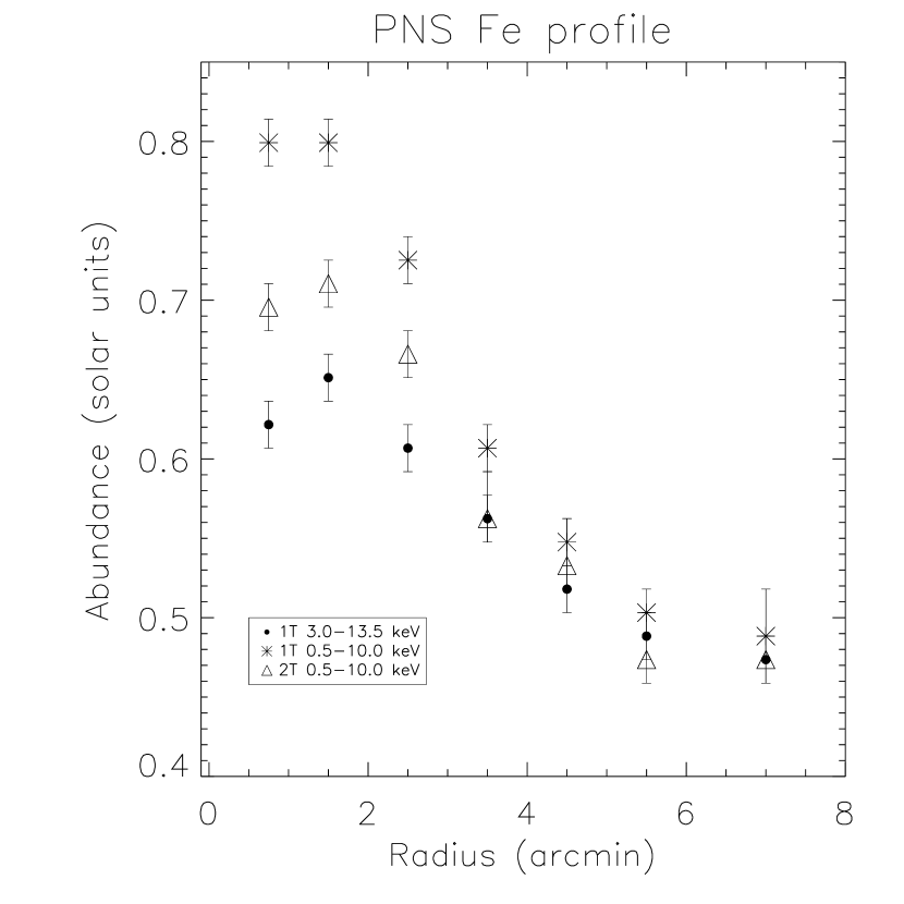
Figure 9: Fe abundance profiles obtained in the entire 0.5-10 keV band using one temperature (crosses) and two temperature models (open triangles) and, for comparison, the one obtained with the best fit model in the hard band (full circles), for PN singles data, on the top, and for MOS2 data, on the bottom. Uncertainties are at the 68% level for one interesting parameter ($\Delta\chi^{2}\,=\,1$).

The Fe abundance profile, shown in Fig 9 is not substantially changed and in particular the abundance gradient is even more evident. Instead for the Ni abundance profile, shown in Fig 10, the evidence for a gradient is not present. In fact adding a linear component improves the fit ($\chi^{2}=1.9$ for 5 d.o.f) respect to a constant ($\chi^{2}=1.9$ for 6 d.o.f) for the PN Ni abundances derived by the 1T model in the hard band, while the Ni profile derived by the 2T model in the entire band is essentially flat (fitting a constant returns a $\chi^{2}=3$ for 6 d.o.f and a linear component does not improve the fit, $\chi^{2}=2.9$ for 6 d.o.f). We caution the reader that the 2T modelization is rather complex, because some not completely justified assumptions are made, as for example that the abundances of the two components are equal, and there is some degeneracy in the contribution of the two X-ray emission components and the soft proton power-law background (see for MOS2 and PN the substantial difference in the temperature of the cool component ). Therefore the derived Ni abundance should be taken with some caution. Moreover it is very difficult to explain, in presence of a confirmed Fe abundance gradient, a flat Ni abundance profile and a Ni/Fe ratio which increases going outward.

5 Discussion

Our main result can be summarized as follows: there is no need to invoke resonant scattering in the Fe He$\alpha$ line in the Perseus cluster core and the Fe abundance determination with optically thin emission models is reliable.

Resonant scattering should be important in the core of galaxy clusters, this is particularly true for the Fe He$\alpha$ line in the core of the Perseus cluster (it has an optical depth of 3.3 according to Sazonov et al. 2002). The optical depth of a resonance line depends on the characteristic velocities of small scale internal motions, which could seriously diminish the depth $\tau$ (Gilfanov et al. 1987, see Mathews et al. 2001 for an example of a detailed calculation in presence of turbulent motions). The absence of a clear evidence of resonant scattering strongly points towards the presence of significant gas motions. In fact, following Gilfanov et al. (1987), the optical depth is

$$\tau=\tau^{0}\,(1+v_{turb}^{2}/v_{Fe}^{2})^{-1/2}$$ (1)

where $\tau^{0}$ is the optical depth at the line center in the absence of turbulence (in spectroscopy the word turbulence is used for all hydrodynamic motions of unknown pattern which cause a broadening of the spectral lines. In hydrodynamics turbulence has a much more restricted meaning), $v_{turb}$ is the turbulent velocity of the gas and $v_{Fe}=(2kT_{e}/M_{Fe})^{1/2}\sim c_{s}/8.8$ is the thermal speed of the iron ions and $c_{s}$ denotes the adiabatic sound speed in the ICM. Thus the absence of resonant scattering, $\tau<1$, and assuming $\tau^{0}=3.3$ (Sazonov et al., 2002), implies gas motions with characteristic velocities greater than $0.36\,c_{s}$, i.e a Mach number $M\gtrsim 0.36$.

Studies of optical line emission in the central regions of ellipticals reveal chaotic gas kinematics typically about 0.2-0.4 of the sound speed in the hot gas (Caon et al., 2000) and since small, optically visible line-emitting regions at T $\sim 10^{4}$ K are likely to be strongly coupled to the ambient gas, as some models predict (Sparks et al., 1989) and clear correlation between H$\alpha$+[N II] and X-ray luminosities suggests, the hot gas should share the same turbulent velocities. The first clear example of resonant scattering, acting on the $2p-3d$ line of Fe XVII at 15.0 Å (0.83 keV), has been recently found in the giant elliptical galaxy NGC 4636 (Xu et al., 2002) using the reflection grating on board XMM-Newton and measuring the cross dispersion profile of the ratio between an optically thin emission blend, the two $2p-3s$ lines of Fe XVII at 17.0-17.1 Å (0.73 keV) and the optically thick line at 15.0 Å. Xu et al. (2002) found that if an average turbulent velocity dispersion more than 1/10 of the sound speed is added to the assumed Maxwellian the model becomes incompatible with the ratio of the 17.1 Å/15.0 Å lines. We remind that the detection of the resonant scattering is only in the inner $1^{\prime}$, in-fact the phenomenon does not affect spectra extracted within a full-width of $2^{\prime}$ (Xu et al., 2002). Another elliptical, NGC 5044, was observed with the RGS (Tamura et al., 2003) and no evidence of resonant scattering was found in spectra extracted in the full $2^{\prime}$. If also in this case a cross dispersion analysis where to show resonant scattering, these would rule out possible associations at least at these inner scales with optically line-emitting gas, because NGC 4636 and NGC 5044 are the most striking examples of chaotic gas kinematics in the sample of Caon et al. (2000).

Another possible source of gas motions is the activity of an AGN, which is now thought to be widespread in the core of galaxy clusters and strongly related to hot bubbles, for which one of the best cases is indeed the Perseus cluster (Fabian et al., 2002). The induced motions could be either turbulent or laminar, as suggested by the recent Chandra and optical results in Fabian et al. (2003a, b) (see the discussion about the flow causing the horseshoe $\rm{H}\alpha$ filament and the derived velocity of 700 $\rm{km\,s^{-1}}$ which for a sound speed of about 1170 $\rm{km\,s^{-1}}$, for a temperature of 5 keV, implies $M\sim 0.6$ or about the sound waves generated by the continuous blowing of bubbles). AGN activity could explain the lack of resonant scattering also in the other best candidate M87 (but see also the discussion suggesting caution for these interpretation in the analysis of RGS data for M87 of Sakelliou et al. 2002).
What is becoming progressively clearer is that resonant scattering effects must be small and confined on small inner scales.

The Fe abundance gradient confirms the general picture of an increase of SNIa ejecta in the center of relaxed cD clusters. The Ni abundance, because Ni is almost exclusively produced by SNIa, and the presence of a gradient also in this element could be a crucial confirmation of this general picture (see De Grandi & Molendi 2002b which report measures of Fe and Ni for a sample of 22 clusters observed with BeppoSAX and in particular their Fig.6 showing a segregation between relaxed cD clusters and not relaxed clusters, with the formers with greater Fe and Ni abundances respect to latters). The Ni abundance gradient is evident in the fit in the high energy band and, looking back at the BeppoSAX data, we can attribute the excess in the 8 keV line complex to an increased Ni abundance. However the complex thermal structure of the gas prevents us from reaching a robust determination of the Ni abundance profile. Detailed temperature and abundances maps are required to address this issue.

Figure 1: PN light curve in the energy band 10-13 keV together with our threshold of 0.35 cts/s.

Figure 2: PN singles temperature profile. Uncertainties are at the 68% level for one interesting parameter($\Delta\chi^{2}\,=\,1$). Full circles represent the temperature obtained using the range 3-10 keV, open triangles the temperature obtained using the range 3-7 keV and open squares the temperature obtained by using the range 3-13.5 keV and adding to the source model a power law background component. In the last two bins we do not show the temperatures obtained in the 3-10 keV and 3-7 keV bands because they are larger than 10 keV. Diamonds represent the temperature obtained by the ratio of the fluxes of He$\alpha$ to H$\alpha$ Fe lines.

Figure 3: Temperature profiles obtained with the various EPIC cameras compared with the temperature profile obtained with the MECS instrument on board BeppoSAX . Uncertainties are at the 68% level for one interesting parameter ($\Delta\chi^{2}\,=\,1$). Crosses represent temperatures obtained with MOS1, open triangles with MOS2, open squares with PN singles, open diamonds with PN doubles and full stars with the MECS.

Figure 4: PN singles data for the $1^{\prime}-2^{\prime}$ bin in the 6-8 keV band and the corresponding fit with a MEKAL model, on the left, and with a VMEKAL model, on the right, together with the corresponding ratios of data respect to models.

Figure 5: Abundance profiles for Fe, on the top, and for Ni, on the bottom, obtained with the various EPIC cameras compared with the abundance profiles obtained with the MECS instrument on board BeppoSAX . Uncertainties are at the 68% level for one interesting parameter ($\Delta\chi^{2}\,=\,1$). As in Fig.3, crosses refers to MOS1, open triangles to MOS2, open squares to PN singles, open diamonds to PN doubles and full stars to MECS.

Figure 6: PN singles data for the $1^{\prime}-2^{\prime}$ bin in the 6-8 keV band and the corresponding fit with an APEC model version 1.3.0, together with the corresponding ratios of data respect to models.

Figure 7: Temperature profiles obtained in the entire 0.5-10 keV band using one temperature (crosses) and two temperature models (open triangles, both the temperatures of the hot and cold component are shown) and, for comparison, the one obtained with the best fit model in the hard band (full circles), for PN singles data, on the top, and for MOS2 data, on the bottom. Uncertainties are at the 68% level for one interesting parameter ($\Delta\chi^{2}\,=\,1$).

Figure 8: Ratio of the normalizations of the two temperature components, obtained by a two temperature model fitted in the 0.5-10 keV band, for PN single data (full circles) and MOS2 data (open triangles). Uncertainties are at the 68% level for one interesting parameter ($\Delta\chi^{2}\,=\,1$).

Figure 10: Ni abundance profiles obtained in the entire 0.5-10 keV band using one temperature (crosses) and two temperature models (open triangles) and, for comparison, the one obtained with the best fit model in the hard band (full circles), for PN singles data, on the top, and for MOS2 data, on the bottom. Uncertainties are at the 68% level for one interesting parameter ($\Delta\chi^{2}\,=\,1$).

Table 1: Parameters values for one and two temperatures models in different energy bands for the inner rings of the Perseus cluster using the single events of the PN camera. All errors quoted are at the 68% level for one interesting parameter ($\Delta\chi^{2}=1$ )

Bin	Mod-Band	$\rm{N_{H}}$	$\rm{kT_{h}}$	$\rm{EM_{h}}$	$\rm{kT_{c}}$	$\rm{EM_{c}}$	Fe	Ni	$\chi^{2}$/d.o.f
0.5′-1′	1T+pow/b (3-13.5 keV)		$3.91^{+0.11}_{-0.04}$	$4.99^{+0.03}_{-0.09}$			$0.62^{+0.01}_{-0.01}$	$1.53^{+0.27}_{-0.24}$	845/809
	1T (3-10 keV)		$3.99^{+0.05}_{-0.06}$	$4.91^{+0.02}_{-0.03}$			$0.62^{+0.01}_{-0.01}$	$1.48^{+0.27}_{-0.24}$	834/799
	1T (0.5-10 keV)	$1.09^{+0.01}_{-0.01}$	$3.29^{+0.01}_{-0.01}$	$5.75^{+0.01}_{-0.01}$			$0.80^{+0.01}_{-0.01}$	$1.38^{+0.11}_{-0.15}$	2037/1299
	2T (0.5-10 keV)	$1.15^{+0.01}_{-0.01}$	$5.00^{+0.08}_{-0.01}$	$3.07^{+0.02}_{-0.03}$	$2.03^{+0.02}_{-0.01}$	$2.90^{+0.04}_{-0.07}$	$0.69^{+0.01}_{-0.01}$	$1.06^{+0.11}_{-0.10}$	1734/1297
1′-2′	1T+pow/b (3-13.5 keV)		$4.01^{+0.04}_{-0.04}$	$11.3^{+0.1}_{-0.1}$			$0.65^{+0.01}_{-0.01}$	$1.23^{+0.16}_{-0.16}$	1114/1051
	1T (3-10 keV)		$4.13^{+0.06}_{-0.02}$	$11.2^{+0.1}_{-0.1}$			$0.64^{+0.01}_{-0.01}$	$1.24^{+0.15}_{-0.17}$	1091/1020
	1T (0.5-10 keV)	$1.12^{+0.01}_{-0.01}$	$3.58^{+0.01}_{-0.01}$	$12.19^{+0.01}_{-0.02}$			$0.80^{+0.01}_{-0.01}$	$1.42^{+0.10}_{-0.09}$	2894/1520
	2T (0.5-10 keV)	$1.17^{+0.01}_{-0.01}$	$4.95^{+0.02}_{-0.03}$	$7.97^{+0.03}_{-0.05}$	$2.04^{+0.01}_{-0.02}$	$4.77^{+0.08}_{-0.03}$	$0.71^{+0.01}_{-0.01}$	$1.16^{+0.06}_{-0.10}$	2371/1518
2′-3′	1T+pow/b (3-13.5 keV)		$4.86^{+0.07}_{-0.04}$	$8.89^{+0.10}_{-0.13}$			$0.61^{+0.01}_{-0.01}$	$0.85^{+0.15}_{-0.17}$	1079/1063
	1T (3-10 keV)		$4.99^{+0.06}_{-0.04}$	$8.83^{+0.07}_{-0.03}$			$0.61^{+0.01}_{-0.01}$	$0.91^{+0.16}_{-0.17}$	1039/1020
	1T (0.5-10 keV)	$1.14^{+0.01}_{-0.01}$	$4.28^{+0.01}_{-0.02}$	$9.74^{+0.01}_{-0.04}$			$0.72^{+0.01}_{-0.01}$	$1.24^{+0.13}_{-0.12}$	2349/1519
	2T (0.5-10 keV)	$1.18^{+0.01}_{-0.01}$	$5.95^{+0.04}_{-0.03}$	$7.22^{+0.03}_{-0.06}$	$2.11^{+0.02}_{-0.01}$	$2.86^{+0.08}_{-0.02}$	$0.67^{+0.01}_{-0.01}$	$1.08^{+0.09}_{-0.12}$	1978/1517
3′-4′	1T+pow/b (3-13.5 keV)		$5.52^{+0.08}_{-0.07}$	$6.44^{+0.04}_{-0.04}$			$0.56^{+0.01}_{-0.01}$	$0.80^{+0.19}_{-0.19}$	1061/1080
	1T (3-10 keV)		$6.03^{+0.08}_{-0.09}$	$6.36^{+0.03}_{-0.03}$			$0.56^{+0.01}_{-0.01}$	$0.87^{+0.16}_{-0.17}$	1062/1027
	1T+pow/b (0.5-10 keV)	$1.15^{+0.01}_{-0.01}$	$4.99^{+0.02}_{-0.03}$	$6.93^{+0.01}_{-0.02}$			$0.61^{+0.01}_{-0.01}$	$1.09^{+0.15}_{-0.15}$	2040/1527
	2T+pow/b (0.5-10 keV)	$1.19^{+0.01}_{-0.01}$	$5.64^{+0.02}_{-0.04}$	$6.25^{+0.03}_{-0.02}$	$1.64^{+0.03}_{-0.01}$	$0.79^{+0.01}_{-0.04}$	$0.56^{+0.03}_{-0.01}$	$1.06^{+0.15}_{-0.12}$	1914/1525
4′-5′	1T+pow/b (3-13.5 keV)		$5.97^{+0.08}_{-0.09}$	$5.67^{+0.08}_{-0.06}$			$0.52^{+0.01}_{-0.01}$	$0.71^{+0.21}_{-0.20}$	1210/1090
	1T+pow/b (0.5-10 keV)	$1.13^{+0.02}_{-0.01}$	$5.57^{+0.02}_{-0.03}$	$5.99^{+0.01}_{-0.02}$			$0.55^{+0.01}_{-0.01}$	$0.81^{+0.18}_{-0.16}$	1960/1521
	2T+pow/b (0.5-10 keV)	$1.19^{+0.01}_{-0.01}$	$6.26^{+0.04}_{-0.03}$	$5.49^{+0.03}_{-0.01}$	$1.61^{+0.03}_{-0.04}$	$0.60^{+0.01}_{-0.03}$	$0.53^{+0.03}_{-0.01}$	$0.78^{+0.11}_{-0.12}$	1877/1519
5′-6′	1T+pow/b (3-13.5 keV)		$6.36^{+0.14}_{-0.11}$	$4.69^{+0.02}_{-0.03}$			$0.49^{+0.01}_{-0.01}$	$0.50^{+0.25}_{-0.24}$	1095/1072
	1T+pow/b (0.5-10 keV)	$1.13^{+0.01}_{-0.01}$	$5.65^{+0.02}_{-0.05}$	$5.06^{+0.01}_{-0.02}$			$0.50^{+0.01}_{-0.01}$	$1.14^{+0.21}_{-0.18}$	2004/1497
	2T+pow/b (0.5-10 keV)	$1.18^{+0.01}_{-0.01}$	$6.36^{+0.06}_{-0.06}$	$4.69^{+0.02}_{-0.01}$	$1.37^{+0.03}_{-0.01}$	$0.42^{+0.01}_{-0.03}$	$0.47^{+0.02}_{-0.01}$	$1.24^{+0.14}_{-0.23}$	1898/1495
6′-8′	1T+pow/b (3-13.5 keV)		$6.78^{+0.13}_{-0.11}$	$7.44^{+0.11}_{-0.20}$			$0.47^{+0.01}_{-0.01}$	$0.12^{+0.23}_{-0.11}$	1249/1289
	1T+pow/b (0.5-10 keV)	$1.15^{+0.01}_{-0.01}$	$5.85^{+0.03}_{-0.04}$	$8.04^{+0.01}_{-0.02}$			$0.49^{+0.03}_{-0.01}$	$0.93^{+0.20}_{-0.17}$	2274/1637
	2T+pow/b (0.5-10 keV)	$1.21^{+0.01}_{-0.01}$	$6.69^{+0.04}_{-0.06}$	$7.50^{+0.02}_{-0.02}$	$1.29^{+0.01}_{-0.03}$	$0.63^{+0.02}_{-0.02}$	$0.47^{+0.01}_{-0.01}$	$1.27^{+0.12}_{-0.23}$	2009/1635

Table 2: Parameters values for one and two temperatures models in different energy bands for the inner rings of the Perseus cluster using the the MOS2 camera. All errors quoted are at the 68% level for one interesting parameter ($\Delta\chi^{2}=1$ )

Bin	Mod-Band	$\rm{N_{H}}$	$\rm{kT_{h}}$	$\rm{EM_{h}}$	$\rm{kT_{c}}$	$\rm{EM_{c}}$	Fe	Ni	$\chi^{2}$/d.o.f
0.5′-1′	1T+pow/b (3-12 keV)		$3.84^{+0.06}_{-0.04}$	$5.36^{+0.02}_{-0.03}$			$0.64^{+0.03}_{-0.01}$	$0.76^{+0.34}_{-0.29}$	385/323
	1T (3-10 keV)		$3.86^{+0.07}_{-0.03}$	$5.37^{+0.02}_{-0.03}$			$0.64^{+0.03}_{-0.01}$	$0.83^{+0.30}_{-0.30}$	372/318
	1T (0.5-10 keV)	$1.17^{+0.01}_{-0.01}$	$3.38^{+0.01}_{-0.02}$	$5.91^{+0.01}_{-0.01}$			$0.81^{+0.01}_{-0.01}$	$1.04^{+0.18}_{-0.09}$	810/479
	2T (0.5-10 keV)	$1.20^{+0.02}_{-0.01}$	$5.18^{+0.05}_{-0.06}$	$2.82^{+0.03}_{-0.09}$	$2.33^{+0.02}_{-0.02}$	$3.26^{+0.25}_{-0.08}$	$0.74^{+0.01}_{-0.01}$	$0.88^{+0.12}_{-0.10}$	669/477
1′-2′	1T+pow/b (3-12 keV)		$4.14^{+0.05}_{-0.06}$	$12.2^{+0.1}_{-0.1}$			$0.72^{+0.01}_{-0.01}$	$0.77^{+0.20}_{-0.21}$	436/393
	1T (3-10 keV)		$4.20^{+0.05}_{-0.05}$	$12.1^{+0.1}_{-0.2}$			$0.71^{+0.01}_{-0.01}$	$0.80^{+0.21}_{-0.20}$	435/379
	1T (0.5-10 keV)	$1.18^{+0.01}_{-0.01}$	$3.67^{+0.01}_{-0.01}$	$13.00^{+0.01}_{-0.02}$			$0.86^{+0.01}_{-0.01}$	$1.09^{+0.11}_{-0.09}$	1228/540
	2T (0.5-10 keV)	$1.19^{+0.01}_{-0.01}$	$6.68^{+0.06}_{-0.09}$	$4.09^{+0.03}_{-0.14}$	$2.91^{+0.01}_{-0.01}$	$9.15^{+0.06}_{-0.05}$	$0.83^{+0.01}_{-0.01}$	$0.98^{+0.11}_{-0.09}$	966/538
2′-3′	1T+pow/b (3-12 keV)		$4.96^{+0.06}_{-0.11}$	$10.00^{+0.15}_{-0.05}$			$0.64^{+0.01}_{-0.01}$	$0.49^{+0.22}_{-0.21}$	406/402
	1T (3-10 keV)		$5.17^{+0.05}_{-0.09}$	$9.83^{+0.12}_{-0.07}$			$0.65^{+0.01}_{-0.02}$	$0.59^{+0.24}_{-0.20}$	415/383
	1T (0.5-10 keV)	$1.17^{+0.01}_{-0.01}$	$4.35^{+0.02}_{-0.01}$	$10.96^{+0.02}_{-0.01}$			$0.72^{+0.01}_{-0.01}$	$1.16^{+0.15}_{-0.11}$	1106/544
	2T (0.5-10 keV)	$1.21^{+0.01}_{-0.01}$	$5.78^{+0.05}_{-0.03}$	$7.84^{+0.05}_{-0.07}$	$2.32^{+0.03}_{-0.02}$	$3.43^{+0.08}_{-0.06}$	$0.69^{+0.01}_{-0.01}$	$0.92^{+0.12}_{-0.10}$	841/542
3′-4′	1T+pow/b (3-12 keV)		$5.78^{+0.09}_{-0.10}$	$7.54^{+0.09}_{-0.07}$			$0.61^{+0.01}_{-0.01}$	$0.81^{+0.26}_{-0.25}$	407/406
	1T (3-10 keV)		$6.15^{+0.09}_{-0.11}$	$7.37^{+0.06}_{-0.05}$			$0.62^{+0.01}_{-0.02}$	$1.03^{+0.26}_{-0.25}$	415/380
	1T+pow/b (0.5-10 keV)	$1.17^{+0.02}_{-0.01}$	$5.25^{+0.04}_{-0.02}$	$7.93^{+0.01}_{-0.01}$			$0.67^{+0.01}_{-0.01}$	$1.17^{+0.22}_{-0.15}$	782/542
	2T+pow/b (0.5-10 keV)	$1.21^{+0.01}_{-0.01}$	$6.30^{+0.05}_{-0.10}$	$5.31^{+0.03}_{-0.08}$	$2.74^{+0.05}_{-0.11}$	$1.47^{+0.14}_{-0.06}$	$0.64^{+0.01}_{-0.02}$	$0.98^{+0.18}_{-0.15}$	687/540
4′-5′	1T+pow/b (3-12 keV)		$6.14^{+0.12}_{-0.17}$	$6.09^{+0.06}_{-0.07}$			$0.55^{+0.01}_{-0.01}$	$0.38^{+0.33}_{-0.30}$	412/401
	1T+pow/b (0.5-10 keV)	$1.26^{+0.01}_{-0.02}$	$5.60^{+0.03}_{-0.04}$	$6.37^{+0.01}_{-0.02}$			$0.58^{+0.01}_{-0.01}$	$1.29^{+0.21}_{-0.23}$	701/538
	2T+pow/b (0.5-10 keV)	$1.27^{+0.02}_{-0.01}$	$6.66^{+0.04}_{-0.11}$	$6.62^{+0.05}_{-0.07}$	$2.36^{+0.06}_{-0.07}$	$1.13^{+0.12}_{-0.04}$	$0.58^{+0.01}_{-0.02}$	$1.23^{+0.19}_{-0.24}$	666/536
5′-6′	1T+pow/b (3-12 keV)		$6.67^{+0.23}_{-0.20}$	$4.83^{+0.06}_{-0.05}$			$0.58^{+0.03}_{-0.03}$	$1.00^{+0.40}_{-0.42}$	363/382
	1T+pow/b (0.5-10 keV)	$1.16^{+0.01}_{-0.01}$	$6.17^{+0.05}_{-0.07}$	$5.01^{+0.02}_{-0.01}$			$0.59^{+0.01}_{-0.03}$	$1.58^{+0.28}_{-0.33}$	650/518
	2T+pow/b (0.5-10 keV)	$1.18^{+0.02}_{-0.02}$	$7.11^{+0.07}_{-0.19}$	$4.22^{+0.05}_{-0.06}$	$3.31^{+0.15}_{-0.18}$	$0.89^{+0.12}_{-0.09}$	$0.59^{+0.01}_{-0.03}$	$1.36^{+0.32}_{-0.27}$	639/516
6′-8′	1T+pow/b (3-12 keV)		$7.20^{+0.21}_{-0.21}$	$7.88^{+0.09}_{-0.09}$			$0.52^{+0.03}_{-0.03}$	$0.46^{+0.40}_{-0.39}$	447/475
	1T+pow/b (0.5-10 keV)	$1.20^{+0.02}_{-0.01}$	$6.50^{+0.06}_{-0.04}$	$8.27^{+0.01}_{-0.02}$			$0.53^{+0.01}_{-0.01}$	$1.17^{+0.28}_{-0.26}$	848/572
	2T+pow/b (0.5-10 keV)	$1.23^{+0.02}_{-0.02}$	$7.98^{+0.09}_{-0.14}$	$6.95^{+0.06}_{-0.18}$	$2.74^{+0.07}_{-0.14}$	$1.46^{+0.23}_{-0.03}$	$0.55^{+0.01}_{-0.01}$	$1.07^{+0.25}_{-0.26}$	798/570

References

- Anders & Grevesse (1989) Anders, E. & Grevesse, N. 1989, Geochimica et Cosmochimica Acta, 53, 197
- Arnaud (1996) Arnaud, K.A., 1996, Astronomical Data Analysis Software and Systems V, eds. Jacoby G. and Barnes J., p17, ASP Conf. Series volume 101
- Arnaud et al. (2001) Arnaud, M., Neumann, D. M., Aghanim, N., Gastaud, R., Majerowicz, S., Hughes, J. P. 2001, A&A, 365, L80
- Caon et al. (2000) Caon, N., Macchetto, d., Pastoriza, M., 2000, ApJS, 127, 39
- Churazov (2003) Churazov, E., 2003, presentation held at the conference The Riddle of Cooling Flows in Galaxies and Clusters of Galaxies, Charlottesville, VA, USA. May 31 – June 4, 2003,
- Costa et al. (2001) Costa, E., Soffitta, P., Bellazzini, R., Brez, A., Lumb, N., Spandre, G., 2001, Nature, 411, 662
- De Grandi & Molendi (2002a) De Grandi, S. & Molendi, S., 2002a, ApJ, 567, 163
- De Grandi & Molendi (2002b) De Grandi, S. & Molendi, S., 2002b, in Chemical Enrichment of Intracluster and Intergalactic Medium, ASP Conference Proceedings Edited by Roberto Fusco-Femiano and Francesca Matteucci. Vol 253, p.3
- Dupke & Arnaud (2001) Dupke, R. A. & Arnaud, K.A., 2001, ApJ, 548, 141
- Fabian et al. (2002) Fabian, A.C., Celotti, A., Blundell, K.M., Kassim, N.E., Perley, R.A., 2002, MNRAS, 331, 369
- Fabian et al. (2003a) Fabian, A.C., Sanders, J.S., Allen, S.W., Crawford, C.S., Iwasawa, K., Johnstone, R.M., Schmidt, R.W., Taylor, G.B., 2003a, MNRAS in press, (astro-ph/030636)
- Fabian et al. (2003b) Fabian, A.C., Sanders, J.S., Crawford, C.S., Conselice, C.J., Gallagher III, J.S., Wyse, R.F.G., 2003b, MNRAS in press, (astro-ph/030639)
- Finoguenov et al. (2002) Finoguenov, A., Matsushita, K., Böhringer, H., Ikebe, Y., Arnaud, M., 2002, A&A, 381, 21
- Freyberg et al. (2002) Freyberg, M.J., Briel, U.G., Dennerl, K., Haberl, F., Hartner, G., Kendziorra, E., Kirsch, M., 2002, in Symp. New visions of the X-ray Universe in the XMM-Newton and Chandra era (ESA SP-488; Noordwijk: ESA)
- Fukazawa et al. (2000) Fukazawa, Y., Makishima, K., Tamura, T., Nakazawa, K., Ezawa, H., Ikebe, Y., Kikuchi, K., Ohashi, T., 2000, MNRAS, 313, 21
- Gastaldello & Molendi (2002) Gastaldello, F. & Molendi, S., 2002, ApJ, 572, 160
- Gastaldello et al. (2003) Gastaldello, F., Ettori, S., Molendi, S., Bardelli, S., Venturi, T., Zucca, E., 2003, A&A in press, (astro-ph/0307342)
- Gilfanov et al. (1987) Gilfanov, M.R., Sunyaev,R.A., Churazov, E.M., 1987, Sov. Astron. Lett., 13, 3
- Grupe (2001) Grupe, D., 2001,
- Grevesse & Sauval (1998) Grevesse, N. & Sauval, A. J., 1998, Space Science Reviews, 85, 161
- Kaastra (1992) Kaastra, J.S., 1992, An X-ray Spectral code for Optically Thin Plasmas (Internal SRON-Leiden Report, updated version 2.0)
- Kaiser (2003) Kaiser, C.R., 2003, MNRAS in press, (astro-ph/0305104)
- Kirsch et al. (2002) Kirsch, M. et al., “Status of the EPIC calibration and data analysis”, 2002, XMM-SOC-CAL-TN-018
- Jansen et al. (2001) Jansen, F., Lumb, D., Altieri, B., Clavel, J., Ehle, M., Erd, C., Gabriel, C., Guainazzi, M., Gondoin, P., Much, R., Munoz, R., Santos, M., Schartel, N., Texier, D., Vacanti, G. 2001, A&A, 365, L1
- Liedahl et al. (1995) Liedahl, D. A., Osterheld A. L., Goldstein, W. H. 1995, ApJ, 438, L115
- Lumb (2002) Lumb, D., “EPIC background files”, 2002, XMM-SOC-CAL-TN-016
- Marty et al. (2002) Marty, P.B., Kneib, J.P., Sadat, R., Ebeling, H., Smail, I., 2002, proceedings SPIE vol. 4851 (astro-ph/0209270)
- Mathews et al. (2001) Mathews, W.G., Buote, D.A., Brighenti, F., 20001, ApJ, 550, L31
- Matsushita et al. (2002) Matsushita, K., Belsole, E., Finoguenov, A., Böhringer, H., 2002, A&A, 386, 77
- Mewe et al. (1985) Mewe, R., Gronenschild, E. H. B. M., van den Oord, G. H. J., 1985, A&AS, 62, 197
- Molendi et al. (1998) Molendi, S., Matt, G., Antonelli, L.A., Fiore, F., Fusco-Femiano, R., Kaastra, J., Maccarone, C., Perola, C., 1998, ApJ, 499, 618
- Molendi et al. (1999) Molendi, S., De Grandi, S., Fusco-Femiano, R., Colafrancesco, S., Fiore, F., Nesci, R., Tamburelli, F., 1999, ApJ, 525, L73
- Molendi (2002) Molendi, S., 2002, ApJ, 580, 815
- Molendi & Sembay (2003) Molendi, S. & Sembay, S., 2003, XMM-SOC-CAL-TN-0036
- Nevalainen et al. (2003) Nevalainen, J., Lieu, R., Bonamente, M., Lumb, D., 2003, ApJ, 584, 716
- Nomoto et al. (1997) Nomoto, K., Iwamoto, K., Nakasato, N., Thielemann, F. K., Brachwitz, F., Tsujimoto, T., Kubo, Y., Kishimoto, N. 1997, Nucl.Phys. A, 621, 467
- Peres et al. (1998) Peres, C.B., Fabian, A.C., Edge, A.C., Allen, S.W., Johnstone, R.M., White, D.A., 1998, MNRAS, 298, 416
- Pratt & Arnaud (2002) Pratt, G.W. & Arnaud, M., 2002, A&A, 394, 375
- Sakelliou et al. (2002) Sakelliou, I., Peterson, J.R., Tamura, T., Paerels, F.B.S., Kaastra, J.S., Belsole, E., Böhringer, H., Branduardi-Raymont, G., Ferrigno, C., den Herder, J.W., Kennea, J., Mushotzky, R.F., Vestrand, W.T., Worrall, D.M., 2002, A&A, 391, 903
- Saxton & Siddiqui (2002) Saxton, R.D. & Siddiqui, H., “The status of the SAS spectral response generation tasks for XMM-EPIC”, 2002, XMM-SOC-PS-TN-43
- Sazonov et al. (2002) Sazonov, S.Yu., Churazov, E.M., Sunyaev, R.A., 2002, MNRAS, 333, 191
- Schmidt et al. (2002) Schmidt, R.W., Fabian, A.C., Sanders, J.S., 2002, MNRAS, 337, 71
- Smith et al. (2001) Smith, R. K., Brickhouse, N. S., Liedahl, D. A., Raymond, J. C. 2001, ApJ, 556, L91
- Sparks et al. (1989) Sparks, W.B., Macchetto, D., Golombeck, D., 1989, ApJ, 345, 153
- Tamura et al. (2003) Tamura, T., Kaastra, J.S., Makishima, K., Takahashi, I., 2003, A&A, 399, 407
- Xu et al. (2002) Xu, H., Kahn, S.M., Peterson, J.R., Behar, E., Paerels, F.B.S., Mushotzky, R.F., Jernigan, J.G., Brinkman, A.C., Makishima, K., 2002, ApJ, 579, 600