A method for relaxing the CFL-condition in time explicit schemes

A method for relaxing the CFL-condition, which limits the time step size in explicit methods in computational fluid dynamics, is presented. The method is based on re-formulating explicit methods in matrix form, and considering them as a special-Jacobi iteration scheme that converge efficiently if the CFL- number is less than unity. By adopting this formulation, one can design various solution methods in arbitrary dimensions that range from explicit to unconditionally stable implicit methods in which CFL-number could reach arbitrary large values. In addition, we find that adopting a specially varying time stepping scheme accelerates convergence toward steady state solutions and improves the efficiently of the solution procedure.

1 Introduction

The majority of the numerical methods used in astrophysical fluid dynamics are based on time-explicit methods (see Stone & Norman, 1992; Ziegler, 1998; Koide et al. 1999, ).
Advancing the solution in time in these methods is based on time-extrapolation procedures, that are found to be numerically stable if the time-step size is shorter than a critical value, which is equivalent to the requirement that the Courant-Friedrich-Levy (CFL) number must be smaller than unity.
This condition, however, limits the range of application and severely affects their robustness (see Fig. 1). Using high performance computers to perform a large number of explicit time steps leads to accumulations of round-off errors that may easily distort the propagation of information from the boundaries and cause divergence of the solution procedure, especially if Neumann type conditions are imposed at the boundaries.
In this paper we present for the first time a numerical strategy toward relaxing the CFL-condition, and therefore enlarging the range of application of explicit methods.

Figure 1: The range of applicability of implicit and explicit methods. The equations describing physical and chemical processes whose characteristic time scales are much shorter than the hydrodynamic time scale ($\tau_{HD}$) should be solved implicitly. For example, the characteristic time corresponding to the propagation of gravitational waves ($\tau_{G}$), peaks in the radiative energy ($\tau_{R}$) and chemical processes ($\tau_{Ch}$) occur on much shorter time scales than $\tau_{HD}.$ In most astrophysical problems $\rm Alfv\acute{e}n$ wave crossing time ($\tau_{MHD}$) is shorter than $\tau_{HD}$. The time scale required for fluid flows (non-relativistic) to relax thermally ($\tau_{Th}$) is in general one order of magnitude larger than $\tau_{HD}$, depending on the efficiency of the cooling processes. However, the viscous time scale ($\tau_{Vis}$) can be significantly larger than $\tau_{HD}$ depending on how large the Reynolds number ($Re$) is. In most astrophysical flows, $Re$ is at least $10^{3}$. If accretion is considered, the time scale for an envelope to evolve ($\tau_{Ev}$) is approximately equal to the mass of the envelope divided by the accretion rate. Thus, for an envelope of $\,{\cal M}_{En}=10^{-5}{\cal M}_{\odot}\,$ to evolve from an accretion rate of $\,\dot{\cal M}\sim 10^{-10}{\cal M}_{\odot}/Y\,$, an accretion time of the order $\,\tau_{Ev}\sim 10^{5}\,$ years is required.

2 Mathematical formulation - scalar case

In fluid flows, the equation of motion which describes the time-evolution of a quantity q in conservation form reads:

$$\frac{\partial q}{\partial t}+L{q}\@vec{V}={f},$$ (1)

where $\@vec{V}$ and $f$ are the velocity field and external forces, respectively. $L$ represents a first and/or second order spatial operator that describe the advection and diffusion of $q$.

In the finite space $\cal{H}$, we may replace the time derivative of $q$ by:

$$\frac{\delta q}{\delta t}=\frac{q^{\mathrm{n+1}}-q^{\mathrm{n}}}{\delta t},$$ (2)

where $q^{\mathrm{n}}$ and $q^{\mathrm{n+1}}$ correspond to the actual value of $q$ at the old and new time levels, respectively.
An explicit formulation of Eq.1 reads:

$$\frac{\delta q}{\delta t}=[-L{q}\@vec{V}+{f}]^{\mathrm{n}},$$ (3)

whereas the corresponding implicit form is:

$$\frac{\delta q}{\delta t}=[-L{q}\@vec{V}+{f}]^{\mathrm{n+1}}.$$ (4)

Combining these two approaches together, we obtain:

$$\frac{\delta q}{\delta t}=\theta[-L{q}\@vec{V}+{f}]^{\mathrm{n+1}}+(1-\theta)[-L{q}\@vec{V}+{f}]^{\mathrm{n}},$$ (5)

where $\theta(0\leq\theta\leq 1)$ is a switch on/off parameter.
To first order in $\delta t$, we may Taylor-expand $q^{n+1}$ and $f^{n+1}$ around $q^{n}$, i.e., $q^{n+1}=q^{n}+\delta q+\mathcal{O}(\delta^{2})$, and obtain:

$$\frac{\delta q}{\delta t}+\theta(L\@vec{V}+{g})\delta q=RHS^{\mathrm{n}},$$ (6)

where $g=\partial f/\partial q$ and $RHS^{\mathrm{n}}=[{f}-L{q}\@vec{V}]^{\mathrm{n}}$. In the following discussion, we term $RHS^{\mathrm{n}}$ as the time-independent residual.
Applying Eq. 6 to the whole number of grid points, the following matrix-equation can be obtained:

$$(\frac{I}{\delta t}+\theta A)\delta q=RHS^{\mathrm{n}}.$$ (7)

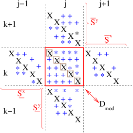
Figure 2: The neighboring block matrices in the x and y-directions resulting from 5-star staggered grid discretization. Entries marked with ‘X’ denote the elements usually used in the implicit operator splitting approach Hujeirat & Rannacher (2001), ‘*’ and ‘+’ are coefficients corresponding to the the source terms. The semi-explicit method for a scalar equation relies on inverting the diagonal matrix whose entries are marked with X surrounded by squares. The generalization of the semi-explicit method to the multi-dimensional HD-equations requires inverting the block diagonal matrix $D_{\mathrm{mod}}$.

The matrix $A$ contains coefficients such as $V/\Delta x$, $\eta/\Delta x^{2}$ and $g$ that correspond to advection, diffusion and to the source terms, respectively. In terms of equation 7, explicit methods are recovered by neglecting the matrix $\theta A$. We note that since the switch parameter $\theta$ does not appear on the RHS of Eq. 7, explicit formulation does not directly depend on $\theta$, but rather on the multiplication of $\theta A$. Thus, for explicit method to converge, it is necessary that the matrix $(\frac{I}{\delta t}+\theta A)$ is diagonally dominant, which implies that $\theta A$ must be negligibly small. In terms of matrix algebra, this means that the absolute value of the sum of elements in each raw of $\theta A$ must be smaller than the corresponding diagonal element $1/{\delta t}$ Hackbusch (1994). In the absence of diffusion and external forces (i.e., $\eta=f=0$), this is equivalent to the requirement that at each grid point: $1/{\delta t}>|V|/\Delta x$, i.e., $CFL\equiv{\delta t}|V|/\Delta x<1$.
On the other hand, the matrix $A$ can be decomposed as follows: $A=D+L+U$, where D is a matrix that consists of the diagonal elements of $A$. L and U contain respectively the sub- and super-diagonal entries of $A$. Noting that a conservative discretization of the advection-diffusion hydrodynamical equations (Navier-Stokes equations) gives rise to a $D$ that contains positive values, we may reconstruct a modified diagonal matrix $D_{\mathrm{mod}}={I}/{\delta t}+\theta D$. In terms of Eq. 7 we obtain:

$$[D_{\mathrm{mod}}+\theta(L+U)]\delta q=RHS^{\mathrm{n}}.$$ (8)

A slightly modified semi-explicit form can be obtained by neglecting the entries of the matrix $\theta(L+U)$. In this case, a necessary condition for the iteration procedure to converge is that the absolute value of the sum of elements in each raw of $\theta(L+U)$ must be much smaller than the corresponding diagonal element of $D_{\mathrm{mod}}$ in the same raw. In terms of Equation 8, the method is said to converge if the entries in each row of $D_{\mathrm{mod}}$ fulfill the following condition:

$$1/{\delta t}+\theta(|V|/\Delta x+\eta/\Delta x^{2}+g)>||A-D||_{\infty},$$ (9)

where $||A-D||_{\infty}$ denotes the $\infty-$norm of $A-D$. This can be achieved, however, if the flow is smooth, viscous, and if appropriate boundary conditions are imposed. Consequently, the inversion process of $D_{\mathrm{mod}}\delta q=RHS^{\mathrm{n}}$ proceeds stably even for large CFL-numbers (see Fig. 5).

Figure 3: The development of the CFL-number (left axis) and the total residual (right axis) versus covered-time in normalized units of five different numerical methods (from to top to bottom: normal explicit, residual smoothing, semi-explicit, implicit operator splitting Hujeirat & Rannacher (2001) and the fully implicit method). While the effective time covered in each run of these different methods is similar, the actual number of iteration is substantially different. The numerical problem here is to search stationary solutions for Taylor flow between two concentric spheres. The inner sphere has a radius $\,r_{in}\!=\!1\,$ and rotates with angular velocity $\,\Omega_{in}\!=\!5\,$, whereas the outer sphere is non-rotating and its radius is taken to be $\,r_{out}\!=\!1.3\,$. We use the viscosity coefficient $\,\nu\!=\!10^{-2}$. The initial density and temperature are taken to be $\,\rho(r,\theta,t\!=\!0)\!=\!1\,$, and $\,T(r,\theta,t\!=\!0)\!=\!10^{1}\,$, respectively. The computational domain is $\,[1,1.3]\times[0,\pi/2]\,$ and consists of $\,30\!\times\!50\,$ non-uniformly distributed tensor-product mesh.

3 Generalization

The set of 2D-hydrodynamical equations in conservative form and in Cartesian coordinates may be written in the following vector form:

$$\frac{\partial\@vec{q}}{\partial t}+L_{\mathrm{x,xx}}\@vec{F}+L_{\mathrm{y,yy}}\@vec{G}=\@vec{f},$$ (10)

where $F$ and $G$ are fluxes of $q$, and $L_{\mathrm{x,xx}},\,L_{\mathrm{y,yy}}$ are first and second order transport operators that describe advection-diffusion of the vector variables $\@vec{q}$ in x and y directions. $\@vec{f}$ corresponds to the vector of source functions.
By analogy with Eq.7, the linearization procedure applied to Eq. 10 yields the following matrix form:

$$[\frac{I}{\delta t}+\theta(AL_{\mathrm{x,xx}}+BL_{\mathrm{y,yy}}-H)]\delta q=RHS^{\mathrm{n}},$$ (11)

where $A=\partial F/\partial q,\,B=\partial G/\partial q$ and $H=\partial\@vec{f}/\partial q$, and which are evaluated on the former time level. $RHS^{\mathrm{n}}=[\@vec{f}-L_{\mathrm{x,xx}}\@vec{F}-L_{\mathrm{y,yy}}\@vec{G}]^{\mathrm{n}}$.
Adopting a five star staggered grid discretization, it is easy to verify that at each grid point Eq. 11 acquires the following block matrix equation:

$$\frac{{\delta q}_{\mathrm{j,k}}}{\delta t}+\underline{S}^{\mathrm{x}}{\delta q}_{\mathrm{j-1,k}}+{D}^{\mathrm{x}}{\delta q}_{\mathrm{j,k}}+\overline{S}^{\mathrm{x}}{\delta q}_{\mathrm{j+1,k}}$$

$$+\underline{S}^{\mathrm{y}}{\delta q}_{\mathrm{j,k-1}}+{D}^{\mathrm{y}}{\delta q}_{\mathrm{j,k}}+\overline{S}^{\mathrm{y}}{\delta q}_{\mathrm{j,k+1}}=RHS^{\mathrm{n}}_{\mathrm{j,k}},$$ (12)

where the underlines (overlines) mark the sub-diagonal (super-diagonal) block matrices in the corresponding directions (see Fig. 2). ${D}^{\mathrm{x,y}}$ are the diagonal block matrices resulting from the discretization of the operators $L_{\mathrm{x,xx}}\@vec{F}$, $L_{\mathrm{y,yy}}\@vec{G}$ and $\@vec{f}$.
To outline the directional dependence of the block matrices, we re-write Eq. 12 in a more compact form:

$$\begin{array}[]{lll}&{\hskip 8.5359pt}\overline{S}^{\mathrm{y}}{\delta q}_{\mathrm{j,k+1}}&\\ +\underline{S}^{\mathrm{x}}{\delta q}_{\mathrm{j-1,k}}&+{D}_{\mathrm{mod}}{\delta q}_{\mathrm{j,k}}&+\overline{S}^{\mathrm{x}}{\delta q}_{\mathrm{j+1,k}}=RHS^{\mathrm{n}}_{\mathrm{j,k}}\\ &+\underline{S}^{\mathrm{y}}{\delta q}_{\mathrm{j,k-1}}.&\end{array}$$ (13)

where ${D}_{\mathrm{mod}}={{\delta q}_{\mathrm{j,k}}}/{\delta t}+{D}^{\mathrm{x}}+{D}^{\mathrm{y}}.$ The subscripts “j” and “k” denote the grid-numbering in the x and y directions, respectively (see Fig. 2).

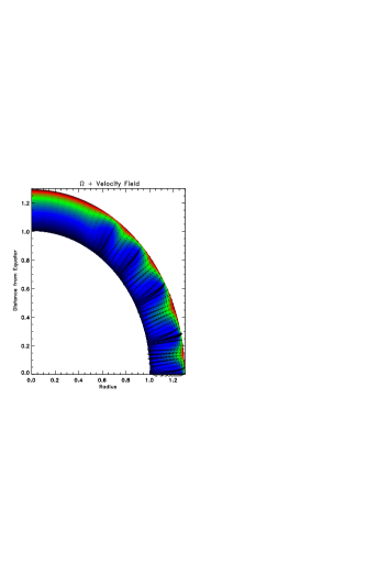
Figure 4: Steady state solutions of the Taylor flow between two concentric spheres. Here the velocity field and the angular velocity (large-to-low values correspond to blue-to-red colors) are shown. The capability of the methods to capture the formation of rotationally-driven multiple vortices near-equatorial region is obvious.

Eq. 13 gives rise to three different types of solution procedures:

1. Classical explicit methods are obviously very special cases that are recovered if all the sub- and super-diagonal block matrices are neglected, as well as ${D}^{\mathrm{x}}$ and ${D}^{\mathrm{y}}$. The only matrix to be retained here is $(1/{\delta t})\,\times\,$(the identity matrix), i.e., the first term on the LHS of Eq. 12. This yields the vector equation:

   $$\frac{{\delta q}_{\mathrm{j,k}}}{\delta t}=RHS^{\mathrm{n}}_{\mathrm{j,k}}.$$ (14)

2. Semi-explicit methods are recovered when neglecting the sub- and super-diagonal block matrices only, but retaining the block diagonal matrices. In this case the matrix equation reads:

   $${D}_{\mathrm{mod}}{\delta q}_{\mathrm{j,k}}=RHS^{\mathrm{n}}_{\mathrm{j,k}}.$$ (15)

   We note that inverting ${D}_{\mathrm{mod}}$ is a straightforward procedure, either analytically or numerically.

3. A fully implicit solution procedure requires retaining all the block matrices on the LHS of Eq. 13. This yields a global matrix that is highly sparse. In this case, the “Approximate Factorization Method” (-AFM: Beam & Warming, 1978) and the “Line Gauss-Seidel Relaxation Method” (-LGS: MacCormack, 1985) are considered to be efficient solvers for the set of equations in multi-dimensions.

Fig. 3 shows the time-development of the CFL-number and the total residual for 5-different solution procedures for searching steady state solutions for Taylor flows between two concentric spheres. Using spherical geometry, the set of the 2D axi-symmetric Navier-Stokes equations are solved. The set consists of the three momentum equations, the continuity and the internal energy equations. The flow is assumed to be adiabatic.
In the explicit case, the equations are solved according to Eq. 14. For the semi-explicit procedure, we solve the HD-equations using the block matrix formulation as described in Equation 15. The implicit operator splitting approach is based in solving each of the HD-equations implicitly. Here the LGS-method is used in the inversion procedure of each equation Hujeirat & Rannacher (2001). Unfortunately, while this method has been proven to be robust for modeling compressible flows with open boundaries, it fails to achieve large CFL-numbers in weakly incompressible flows (Fig. 3). This indicates that pressure gradients in weakly incompressible flows do not admit splitting, and therefore they should be included in the solution procedure simultaneously on the new time level.
In the final case, the whole set of HD-equations taking into account all pressure terms is solved in a fully implicit manner (Fig. 3/bottom). Here we use the AFM for solving the general matrix-equation which is locally described by Eq. 13.
For constructing the time step size in these calculations, we have adopted the following description: $\delta t=\alpha_{0}\epsilon/\max(RHS_{j,k})$, where $\epsilon={\min}(\Delta X_{j},\Delta Y_{k}),$ and where $\alpha_{0}$ is a constant of order unity. The maximum and minimum functions here run over the whole number of grid points.

Figure 5: The semi-explicit method applied to a scalar problem. The Figure shows the development of the CFL-number (left axis) and the residual (right axis) of the angular momentum equation in two dimensions versus the iteration number. As initial conditions we use the steady distributions of the physical variables that have been obtained from the simulations of the Taylor problem (see Fig. 4). This includes the velocity field, density, temperature and $\eta$. For the angular velocity we use $\Omega=0$ as initial condition.

3.1 The specially varying time stepping scheme for accelerating convergence

Let [a,b] be the interval on which Eq. 1 is to be solved. We may divide [a,b] into N equally spaced finite volume cells: $\Delta x_{\mathrm{i}}=(b-a)/N$, $i=1,\,N$. To follow the time-evolution of q using a classical explicit method, the time step size must fulfill the CFL-condition, which requires ${\delta t}$ to be smaller than the critical value: ${\delta t}^{\mathrm{u}}_{\mathrm{c}}={\min}\{\Delta x_{\mathrm{i}}/(V+V_{\mathrm{S}})_{\mathrm{i}}\}$.
If [a,b] is divided into N highly stretched finite volume cells, for example $\Delta x_{\mathrm{1}}<\Delta x_{\mathrm{2}}...<\Delta x_{\mathrm{N}}$, then the CFL-condition restrict the time step size to be smaller than ${\delta t}^{\mathrm{nu}}_{\mathrm{c}}={\min_{i}}\{(\Delta x_{\mathrm{i}}/(V+V_{\mathrm{S}})_{\mathrm{i}}\}$, which is much smaller than ${\delta t}^{\mathrm{u}}_{\mathrm{c}}$. Thus, applying a conditionally stable method to model flows using a highly non-uniform distributed mesh has the disadvantage that the time evolution of the variables in the whole domain are artificially and severely affected by the flow behaviour on the finest cells.
Moreover, advancing the variables in time may stagnate if the flow is strongly or nearly incompressible. In this case, $V_{\mathrm{S}}>>V,$ which implies that the time step size allowed by the CFL-condition approaches zero.
However, we may associate still a time step size with each grid point, e.g., ${\delta t}^{\mathrm{nu}}_{\mathrm{i}}=\Delta x_{\mathrm{i}}/(V+V_{\mathrm{S}})$, and follow the time evolution of each variable $q_{\mathrm{i}}$ independently. Interactions between variables enter the solution procedure through the evaluation of the spatial operators on the former time level. This method, which is occasionally called the “Residual Smoothing Method” proved to be efficient at providing quasi-stationary solutions within a reasonable number of iteration, when compared to normal explicit methods. (Fig. 3, also see Enander, 1997). The main disadvantage of this method is its inability to provide physically meaningful time scales for features that possess quasi-stationary behaviour. Here we suggest to use the obtained quasi-stationary solutions as initial configuration and re-start the calculations using a uniform and physically well defined time step size.

4 Summary

In this letter we have presented a strategy for relaxing the CFL-condition which enlarges the range of application of explicit methods and improve their robustness. The method is based on re-formulating explicit methods in matrix-form, which can be then gradually modified up to a fully implicit scheme. The matrix corresponding to the semi-explicit scheme presented here is a block diagonal matrix that can be easily inverted, either analytically or numerically. Unlike normal explicit methods, in which the inclusion of diffusion limits further the time step size, in the semi-explicit formulation presented here diffusion pronounces the diagonal dominance and enhances the stability of the inversion procedure, irrespective of the dimensionality of the problem. We note that the CFL-numbers achieved in the present modeling of Taylor flows are, indeed, larger than unity, but they are not impressively large as we have predicted theoretically. We may attribute this inconsistency to three different effects: 1) The flow considered here is weakly incompressible. This means that the acoustic perturbations have the largest propagation speeds, which requires that all pressure effects should be included in the solution procedure simultaneously on the new time level. 2) The conditions imposed on the boundaries are non-absorbing, and do not permit advection of errors into regions exterior to the domain of calculations. 3) The method requires probably additional improvements in order to achieve large CFL-numbers. This could be done, for example, within the context of the “defect-correction’ iteration procedure, in which the block diagonal matrix $D_{\mathrm{mod}}$ is employed as a pre-conditioner.

Finally, we have shown that the residual smoothing approach improves the convergence of explicit methods.

References

- Beam & Warming (1978) Beam, R.M., Warming, R.F., 1978, AIAA, 16, 393
- Enander (1997) Enander, R., 1997, SIAM J. Sc. Comp., 18, 5, 1243
- Hackbusch (1994) Hackbusch, W., 1994, “ Iterative Solution of Large Sparse Systems of Equations”, Springer-Verlag, New York-Berlin-Heidelberg
- Hujeirat & Rannacher (2001) Hujeirat, A., Rannacher, R., 2001, New Ast. Reviews, 45, 425
- (5) Koide, S., Shibata K., Kudoh, T., 1999, ApJ, 522, 727
- Stone & Norman (1992) Stone, J.M., Norman, M.L., 1992, ApJS, 80, 753
- Ziegler (1998) Ziegler, U., 1998, Comp. Phys. Comm., 109, 111
- MacCormack (1985) MacCormack, R.W., 1985, AIAA, Paper 85-0032