Constraints on a Cardassian model from SNIa data – revisited

Abstract

We discuss some observational constraints, resulting from SN Ia observations, imposed on the behavior of the original flat Cardassian model, and its extension with the curvature term included. We test the models using the Perlmutter SN Ia data as well as the new Knop and Tonry samples. We estimate the Cardassian model parameters using the best-fitting procedure and the likelihood method. In the fitting procedure we use density variables for matter, Cardassian fluid and curvature, and include the errors in redshift measurement. For the Perlmutter sample in the non-flat Cardassian model we obtain the high or normal density universe ($\Omega_{\mathrm{m},0}\geq 0.3$), while for the flat Cardassian model we have the high density universe. For sample A in the high density universe we also find the negative values of estimates of $n$ which can be interpreted as the phantom fluid effect. For the likelihood method we get that a nearly flat universe is preferred. We show that, if we assume that the matter density is $0.3$, then $n\approx 0$ in the flat Cardassian model, which corresponds to the Perlmutter model with the cosmological constant. Testing with the Knop and Tonry SN Ia samples show no significant differences in results.

I Introduction

Freese and Lewis (2002) have recently proposed an alternative to the cosmological constant model explaining the currently accelerating Universe. In this model the standard Friedmann-Robertson-Walker (FRW) equation is modified by the presence of an additional term $\rho^{n}$, namely

$$H^{2}=\frac{\rho}{3}+B\rho^{n},$$ (1)

where $H\equiv\dot{a}/a$ is the Hubble parameter, $a$ is the scale factor, $\rho$ is the energy density of matter and radiation, and $B$ is a positive constant. For simplicity it is assumed that, the density parameter for radiation matter $\Omega_{\mathrm{r},0}=0$. This proposal seems to be attractive because the expansion of the universe is accelerated automatically due to the presence of the additional term (if we put $B=0$ then the standard FRW equation is recovered).

Because the Cardassian model offers an alternative to the cosmological constant model, the agreement of this model with available observations of type Ia supernovae (SN Ia) was immediately verified (Zhu and Fujimoto, 2003; Sen and Sen, 2003). Some interesting results on observational constraints in the generalized Cardassian model were also obtained from the statistical analysis of gravitational lensed quasars (Dev et al., 2003). In our analysis we use three SN Ia data sets compiled by Perlmutter et al. (1999), Knop et al. (2003) and Tonry et al. (2003) to test both the original Cardassian model and its extension with a curvature term. Our results are inconsistent with Zhu and Fujimoto (2003)’s prediction of the low density Universe. The noteworthy results from the joint analysis of SN Ia data and CMBR were obtained by Sen and Sen (2003) who also confirmed the prediction of low density Universe, but their analysis was restricted to the case of $n>0$. This case was also examined by Frith (2003) who used the Tonry SN Ia data. However, such a choice of an interval for this parameter is not physically justified and both negative and positive values are admissible.

II Basic equation

We add a curvature term to the original Cardassian model. Then equation (1) assumes the following form

$$H^{2}=\frac{\rho}{3}+B\rho^{n}+\frac{k}{a^{2}}.$$ (2)

It is useful to rewrite equation (2) in dimensionless variables $\Omega_{i,0}$, $i=(\mathrm{m},\mathrm{Card},k)$,

$$\frac{H^{2}}{H_{0}^{2}}=\Omega_{\mathrm{m},0}\left(\frac{a}{a_{0}}\right)^{-3}+\Omega_{\mathrm{Card},0}\left(\frac{a}{a_{0}}\right)^{-3n}+\Omega_{k,0}\left(\frac{a}{a_{0}}\right)^{-2},$$ (3)

where energy density for the dust is assumed ($p=0$) (and hence $\rho\propto a^{-3}$ from a conservation equation), $\Omega_{\mathrm{m},0}$ is the matter density parameter; $\Omega_{\mathrm{Card},0}=3B\rho^{n}/3H_{0}^{2}$ is the density parameter for the fictitious noninteracting fluid which mimics term $\rho^{n}$ and yields additional density in the model. The subscript zero denotes a present value of model parameters. Then

$$\dot{\rho}=-3H(\rho+p)$$ (4)

For $a=a_{0}$ (the present value of scale factor) we obtain the following constraint

$$\Omega_{\mathrm{m},0}+\Omega_{\mathrm{Card},0}+\Omega_{k,0}=1.$$ (5)

For the fictitious Cardassian fluid we obtain $p=(n-1)\rho$ if $\rho\propto a^{-3}$. In this interpretation the negative value of $n$ is equivalent to the existence of phantom matter with supernegative presssure.

Let us note that in the analogous equation describing FRW dynamics with dust and additional fictitious fluid with the equation of state $p=(n-1)\rho$ presented in Sen and Sen (2003) only case $n>0$ was considered.

III Magnitude-redshift relation

It is well known that various cosmic distance measures, for example the luminosity distance, depend sensitively both on the spatial geometry (curvature) and dynamics. Therefore, luminosity depends on the present densities of the different components of matter content and its equation of state. For this reason, the magnitude-redshift relation for distant objects is proposed as a potential test for cosmological models and plays an important role in determining cosmological parameters.

Let us consider an observer located at $r=0$ at the moment $t=t_{0}$ who receives light emitted at $t=t_{1}$ from a source of absolute luminosity $L$ located at the radial distance $r_{1}$. It is known that the cosmological redshift $z$ of the source is related to $t_{1}$ and $t_{0}$ by the relation $1+z=a(t_{0})/a(t_{1})$. If the apparent luminosity $l$ of the source measured by the observer is defined by

$$l=\frac{L}{4\pi d_{L}^{2}}$$ (6)

then the luminosity distance $d_{L}$ of the source is

$$d_{L}=(1+z)a_{0}r_{1}.$$ (7)

For historical reasons, the observed and absolute luminosities are defined in terms of K-corrected observed magnitudes and absolute magnitudes $m$ and $M$, respectively ($l=10^{-2m/5}\cdot 2.52\cdot 10^{-5}\,\mathrm{erg}\,\mathrm{cm}^{-2}\,\mathrm{s}^{-2}$, $L=10^{-2M/5}\cdot 3.02\cdot 10^{35}\,\mathrm{erg}\,\mathrm{s}^{-2}$) (Weinberg, 1972). When written in terms of $m$ and $M$, equation (6) yields

$$m(z,\mathcal{M},\Omega_{\mathrm{m},0},\Omega_{\mathrm{Card},0},\Omega_{k,0})=\mathcal{M}+5\log_{10}[\mathcal{D}_{L}(z,\Omega_{\mathrm{m},0},\Omega_{\mathrm{Card},0},\Omega_{k,0})]$$ (8)

where

$$\mathcal{M}=M-5\log_{10}H_{0}+25$$ (9)

and

$$\mathcal{D}_{L}(z,\Omega_{\mathrm{m},0},\Omega_{\mathrm{Card},0},\Omega_{k,0})\equiv H_{0}d_{L}(z,\Omega_{\mathrm{m},0},\Omega_{\mathrm{Card},0},\Omega_{k,0},H_{0})$$ (10)

is the dimensionless luminosity distance while $d_{L}$ is in Mpc.

The standard analysis yields the following relationship for the dimensionless luminosity distance

$$\mathcal{D}_{L}((z,\Omega_{\mathrm{m},0},\Omega_{\mathrm{Card},0},\Omega_{k,0})=\frac{(1+z)}{\sqrt{\mathcal{K}}}\xi\left(\sqrt{\mathcal{K}}\int\limits_{0}^{z}[(1-\Omega_{\mathrm{m},0}-\Omega_{\mathrm{Card},0})(1+z^{\prime})^{2}\right.\\ \left.\phantom{\int\limits_{0}^{z}}+\Omega_{\mathrm{m},0}(1+z^{\prime})^{3}+\Omega_{\mathrm{Card},0}(1+z^{\prime})^{3n}]^{-1/2}dz^{\prime}\right),$$ (11)

where

$$\xi(x) =\sin x \mathrm{with} \mathcal{K} =-\Omega_{k,0} \mathrm{when} \Omega_{k,0} <0$$

$$\xi(x) =x \mathrm{with} \mathcal{K} =1 \mathrm{when} \Omega_{k,0} =0$$ (12)

$$\xi(x) =\sinh x \mathrm{with} \mathcal{K} =\Omega_{k,0} \mathrm{when} \Omega_{k,0} >0$$

and the density parameter for hypothetical curvature fluid is

$$\Omega_{k,0}=-\frac{k}{\dot{a}_{0}^{2}}.$$

Thus, for given $\mathcal{M}$, $\Omega_{\mathrm{m},0}$, $\Omega_{\mathrm{Card},0}$, $\Omega_{k,0}$, equations (8) and (11) give the predicted value of $m(z)$ at a given $z$.

The goodness of fit is characterized by the parameter

$$\chi^{2}=\sum_{i}\frac{|\mu_{0,i}^{0}-\mu_{0,i}^{t}|}{\sigma_{\mu 0,i}^{2}+\sigma_{\mu z,i}^{2}}$$ (13)

where $\mu_{0,i}^{0}$ is the measured value, $\mu_{0,i}^{t}$ is the value calculated in the model described above, $\sigma_{\mu 0,i}^{2}$ is the measurement error, $\sigma_{\mu z,i}^{2}$ is the dispersion in the distance modulus due to peculiar velocities of galaxies.

We assume that supernovae measurements come with uncorrelated Gaussian errors and in this case the likelihood function $\mathcal{L}$ can be determined from a chi-squared statistic $\mathcal{L}\propto\exp{(-\chi^{2}/2)}$ (Perlmutter et al., 1999; Riess et al., 1998).

IV Statistical analysis with the Perlmutter sample

We have decided to test our model using the Perlmutter samples of supernovae (Perlmutter et al., 1999). We estimate the value of $\mathcal{M}$ (equation (9)) separately for the full sample of 60 supernovae (sample A) and for the sample of 54 supernovae (sample C — in that sample we exclude 2 supernovae as outliers and 2 as likely reddened ones from the sample of 42 high redshift supernovae and 2 outliers from the sample of 18 low redshift supernovae). We obtain the value of $\mathcal{M}=-3.39$ for sample A, and $\mathcal{M}=-3.43$ for sample C. To test the model we calculate the best fit with minimum $\chi^{2}$ as well as estimate the model parameters using the likelihood method (Riess et al., 1998). For both statistical methods we take the parameter $n$ in the interval $[-3.33,2]$, $\Omega_{\mathrm{m},0}$ in the interval $[0,1]$, $\Omega_{k,0}$ in the interval $[-1,1]$, while an interval for $\Omega_{\mathrm{Card},0}$ is obtained from equation (5).

First, we estimate best fitting parameters for the non-flat Cardassian model and obtain $\Omega_{k,0}=-1.00$, $\Omega_{\mathrm{m},0}=0.83$, $n=-0.67$, $\Omega_{\mathrm{Card},0}=1.17$ for sample A, and $\Omega_{k,0}=-1.00$, $\Omega_{\mathrm{m},0}=0.60$, $n=0.50$, $\Omega_{\mathrm{Card},0}=1.40$ for sample C. This model is characterized with strong negative curvature, that is similar to the Perlmutter results. Let us note that such a high value of $\Omega_{k,0}$ is in contradiction with CMB observations, which prefer the flat universe. When we assume that $\Omega_{k,0}=0$ then we obtain the best-fitted flat Cardassian model with $\Omega_{\mathrm{m},0}=0.52$, $n=-0.93$, $\Omega_{\mathrm{Card},0}=0.48$ for sample A, and $\Omega_{\mathrm{m},0}=0.46$, $n=-0.60$, $\Omega_{\mathrm{Card},0}=0.54$ for sample C. The detailed values are in Tables 1 and 2.

Table 1: Results of the statistical analysis of the Cardassian model obtained both for Perlmutter sample A and C from the best fit with minimum $\chi^{2}$ (denoted with BF) and from the likelihood method (denoted with L). The same analysis was repeated with fixed $\Omega_{\mathrm{m},0}=0.3$.

sample	$\Omega_{\mathrm{Card}}$	$\Omega_{k,0}$	$\Omega_{\mathrm{m},0}$	$n$	$\mathcal{M}$	$\chi^{2}$	method
A	1.17	-1.00	0.83	-0.67	-3.39	94.8	BF
	0.37	-0.12	0.50	-0.13	-3.39	—	L
	1.65	-0.95	0.30	0.37	-3.39	95.7	BF
	0.27	0.45	0.30	0.33	-3.39	—	L
C	1.40	-1.00	0.60	0.50	-3.43	52.8	BF
	0.33	0.17	0.29	0.10	-3.43	—	L
	1.70	-1.00	0.30	0.36	-3.43	53.2	BF
	0.29	0.41	0.30	0.30	-3.43	—	L

Table 2: Results of the statistical analysis of the Cardassian flat model for Perlmutter sample A and sample C obtained both from the best fit with minimum $\chi^{2}$ (denoted with BF) and from the likelihood method (denoted with L). In the case in which we marginalize over $\mathcal{M}$ we denote it with $\mathcal{M}$. The same analysis was repeated with fixed $\Omega_{\mathrm{m},0}=0.3$.

sample	$\Omega_{\mathrm{Card},0}$	$\Omega_{\mathrm{m},0}$	$n$	$\mathcal{M}$	$\chi^{2}$	method
A	0.48	0.52	-0.93	-3.39	95.3	BF
	0.40	0.60	-0.53	-3.39	—	L
	0.46	0.54	-1.43	-3.44	95.0	$\mathcal{M}$, BF
	0.46	0.54	-1.20	-3.41	—	$\mathcal{M}$, L
	0.70	0.30	0.03	-3.39	96.1	BF
	0.70	0.30	0.03	-3.39	—	L
	0.70	0.30	0.03	-3.39	96.1	$\mathcal{M}$, BF
	0.70	0.30	0.03	-3.39	—	$\mathcal{M}$, L
C	0.54	0.46	-0.60	-3.43	95.3	BF
	0.42	0.58	0.10	-3.43	—	L
	0.52	0.48	-0.96	-3.46	95.0	$\mathcal{M}$, BF
	0.48	0.52	0.17	-3.45	—	$\mathcal{M}$, L
	0.7	0.30	-0.03	-3.43	53.3	BF
	0.7	0.30	-0.03	-3.43	—	L
	0.7	0.30	-0.03	-3.43	53.3	$\mathcal{M}$, BF
	0.7	0.30	-0.03	-3.43	—	$\mathcal{M}$, L

For sample C we draw the best-fitted, non-flat (upper-middle curve), flat (lower-middle curve) Cardassian models as well as the best-fitted Perlmutter model with $\Omega_{\mathrm{m},0}=0.28$, $\Omega_{\Lambda,0}=0.72$ (upper curve) against to the flat Einstein-de Sitter model (zero line) on the Hubble diagram (Fig. 1). One can observe that the difference between the best-fitted Cardassian model and the Einstein-de Sitter model with $\Omega_{\Lambda,0}=0$ assumes the largest value for $z\sim 0.9$ and significantly decreases for higher redshifts. While the best-fitted flat Cardassian model and Perlmutter one have increasing differences to the flat Einstein-de Sitter model for higher redshifts, the differences between the best-fitted flat Cardassian model and Perlmutter model increase for higher redshifts. It gives us a possibility to discriminate between the Perlmutter model and Cardassian models if $z\simeq 1$ supernovae data will be available. It is very important because for the present data the Cardassian models are only marginally better than the Perlmutter model.

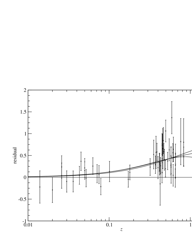
Figure 1: Residuals (in mag) between the Einstein-de Sitter model and four cases: the Einstein-de Sitter itself (zero line), the Perlmutter flat model (upper curve), the best-fitted flat Cardassian model (upper-middle curve), $\Omega_{k,0}=0$, $\Omega_{\mathrm{m},0}=0.46$, $n=-0.60$, $\Omega_{\mathrm{Card},0}=0.54$ and the best-fitted (non-flat) Cardassian model (lower-middle curve) $\Omega_{k,0}=-1.00$, $\Omega_{\mathrm{m},0}=0.60$, $n=0.50$, $\Omega_{\mathrm{Card},0}=1.40$.

However, knowing the best-fit values alone has no enough scientific relevance, if confidence levels for parameter intervals are not presented, too. Therefore, we carry out the model parameters estimation using the minimization procedure, based on the likelihood method. On the confidence level $68.3\%$ we obtain parameter values for samples A and C (Table 3).

Table 3: Non-flat Cardassian model parameter values obtained from the minimization procedure carried out on the Perlmutter samples.

sample	$\Omega_{k,0}$	$\Omega_{\mathrm{Card},0}$	$\Omega_{\mathrm{m},0}$	$n$
A	$-0.12^{+0.54}_{-0.50}$	$0.37^{+0.38}_{-0.20}$	$0.50^{+0.28}_{-0.32}$	$-0.13^{+0.56}_{-1.37}$
C	$0.17^{+0.44}_{-0.66}$	$0.33^{+0.43}_{-0.17}$	$0.29^{+0.28}_{-0.28}$	$0.10^{+0.36}_{-1.46}$

It should be noted that values obtained in both methods are different but the minimization procedure seem to be more adequate for analyzing our problem. The density distributions $f(\Omega_{k,0})$ and $f(n)$ in the Cardassian model are presented on Fig. 2 and 3, respectively. These figures show that the preferred model of the Universe is the nearly flat one, that is in agreement with CMBR data. For sample C the most probable value of $\Omega_{\mathrm{m},0}$ is $0.29$ that is in agreement with the present CMBR and extragalactic data (Peebles and Ratra, 2003; Lahav, 2002). Therefore, the detailed analysis of the flat case of the Cardassian model is carried out.

Figure 2: The density distribution for $\Omega_{k,0}$ in the Cardassian model (sample C). We obtain that $\Omega_{k,0}=0.17^{+0.46}_{-0.66}$ on the confidence level $68.3\%$ (the inner dash lines). Both positive and negative values of $\Omega_{k,0}$ are formally possible.

Figure 3: The density distribution for $n$ in the Cardassian model (sample C). We obtain that $n=0.10^{+0.36}_{-1.46}$ on the confidence level $68.3\%$ (the inner dash lines). Both positive and negative values of $n$ are formally possible.

In the Fig. 4 we presented confidence levels on the plane $(\Omega_{\mathrm{m},0},n)$ minimized over $\mathcal{M}$ for the flat Cardassian model. Figure 4 shows the preferred values of parameters $\Omega_{\mathrm{m},0}$ and $n$. We find that the expected value of $\Omega_{\mathrm{m},0}$ increases when $n$ decreases. The similar result was already obtained by Sen and Sen (2003), for $n>0$. It should be pointed out that these authors argued that $\Omega_{\mathrm{m},0}$ could be less than $0.3$ from the confidence level obtained from the joint analysis of supernovae data and the positions of the CMBR peaks. In the Cardassian model the structure formation would be significantly different from, e.g., the classical model with the cosmological constant. Consequently, in order to calculate the consequence for the CMB the simple angular rescaling does not suffice.

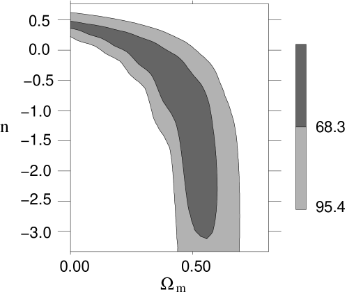
Figure 4: Confidence levels on the plane $(\Omega_{\mathrm{m},0},n)$ minimized over $\mathcal{M}$ for the flat model ($\Omega_{k,0}=0$), and with $\Omega_{\mathrm{Card},0}=1-\Omega_{\mathrm{m},0}$. The figure shows of the preferred value of $\Omega_{\mathrm{m},0}$ and $n$.

The detailed results of our analysis for the flat model are summarized in Table 2. The best fit procedure suggests that $n$ should be negative and consequently $\Omega_{\mathrm{m},0}$ is greater than $0.3$. While we find the parameter $n$ is negative for minimum value of $\chi^{2}$ statistic, the confidence levels allows the positive values of $n$. For the maximum likelihood method on sample A we obtain that $\Omega_{\mathrm{m},0}=0.60^{+0.06}_{-0.15}$ and $n=-0.53^{+0.86}_{-1.27}$ on the confidence level $68.3\%$ for $\mathcal{M}=-3.39$; while $\Omega_{\mathrm{m},0}=0.54^{+0.10}_{-0.11}$ and $n=-1.20^{+0.53}_{-1.36}$ on the confidence level $68.3\%$ when we marginalize over $\mathcal{M}$.

In turn for sample C we obtain that $\Omega_{\mathrm{m},0}=0.58^{+0.06}_{-0.13}$ and $n=0.10^{+0.30}_{-1.57}$ on the confidence level $68.3\%$ for $\mathcal{M}=-3.43$ (Fig. 5 and 6), while $\Omega_{\mathrm{m},0}=0.52^{+0.10}_{-0.13}$ and $n=0.17^{+0.20}_{-2.04}$ on the confidence level $68.3\%$ when we marginalize over $\mathcal{M}$.

Figure 5: The density distribution for $\Omega_{\mathrm{m},0}$ in the Cardassian flat model. We obtain that $\Omega_{\mathrm{m},0}=0.58^{+0.06}_{-0.13}$ on the confidence level $68.3\%$ (the inner dash lines). Additionally the confidence level $95.4\%$ is marked (the outer dash lines).

Figure 6: The density distribution for $n$ in the Cardassian flat model. We obtain that $n=0.10^{+0.30}_{-1.57}$ on the confidence level $68.3\%$ (the inner dash lines). Additionally the confidence level $95.4\%$ is marked (the outer dash lines). Both positive and negative values of $n$ are formally possible.

For the flat model with $\Omega_{\mathrm{m},0}=0.3$ we obtain for sample A $n=-0.03$ with $\sigma(n)=0.13$ both for $\mathcal{M}=-3.39$ and with $\sigma(n)=0.33$ when we marginalize over $\mathcal{M}$. In turn for sample C we obtain that $n=0.03$ with $\sigma(n)=0.12$ both for $\mathcal{M}=-3.43$ (Fig. 7) and $\sigma(n)=0.23$ when we marginalize over $\mathcal{M}$.

Figure 7: The density distribution for $n$ in the Cardassian flat model with $\Omega_{\mathrm{m},0}=0.3$. We obtain that $n=0.03$ with $\sigma(n)=0.12$. Both positive and negative values of $n$ are formally possible.

V Statistical analysis with the Knop sample

Because the Perlmutter sample was completed four years ago, it would be interesting to use newer supernovae observations. Lately Knop et al. (2003) have reegzamined the Permutter sample with host-galaxy extinction correctly applied. They chose from the Perlmutter sample these supernovae which were the more securely spectrally identified as type Ia and have reasonable color measurements. They also included eleven new high redshift supernovae and a well known sample with low redshift supernowae.

We have also decided to test the Cardassian model using this new sample of supernovae. They distinguished a few subsets of supernovae from this sample. We consider two of them. The first is a subset of 58 supernovae with extinction correction (Knop subsample 6; hereafter K6) and the second one of 54 supernovae with low extinction (Knop subsample 3; hereafter K3). Sample C and K3 are similarly constructed because both contain only low extinction supernovae.

It should be pointed out that in contrast to Perlmutter et al. (1999) who included errors in measurement of redshift $z$ Knop et al. (2003) took only uncertainties in the redshift due to peculiar velocities. It is the reason that for security we separately repeated our analysis including errors in measurement of redshift $z$ (subsamples K6z and K3z). The errors was taken from Perlmutter et al. (1999). In the case when errors were not available we assume $\sigma(z)=0.001$. As one can see above, this change has only marginal influence on the results.

At first we estimate the value of $\mathcal{M}$ (equation (9)) separately for both sample K6 and K3. We obtain the value of $\mathcal{M}=-3.53$ for sample K6, and $\mathcal{M}=-3.48$ for sample K3. It is in agreement with Knop et al. (2003).

First, we estimate best fitting parameters for non-flat Cardassian model and obtain $\Omega_{k,0}=-0.24$, $\Omega_{\mathrm{m},0}=0.65$, $n=-1.10$, $\Omega_{\mathrm{Card},0}=0.59$ for sample K6, and $\Omega_{k,0}=-0.36$, $\Omega_{\mathrm{m},0}=0.49$, $n=-0.20$, $\Omega_{\mathrm{Card},0}=0.87$ for sample K3. When we assume that $\Omega_{k,0}=0$ (flat universe) then we obtain the best-fitted flat Cardassian model with $\Omega_{\mathrm{m},0}=0.53$, $n=-1.50$, $\Omega_{\mathrm{Card},0}=0.47$ for sample K6, and $\Omega_{\mathrm{m},0}=0.41$, $n=-0.63$, $\Omega_{\mathrm{Card},0}=0.59$ for sample K3. The detailed values are in Tables 4 and 5.

Table 4: Results of the statistical analysis of the Cardassian model obtained both for the Knop samples from the best fit with minimum $\chi^{2}$ (denoted with BF) and from the likelihood method (denoted with L). The same analysis was repeated with fixed $\Omega_{\mathrm{m},0}=0.3$.

sample	$\Omega_{\mathrm{Card}}$	$\Omega_{k,0}$	$\Omega_{\mathrm{m},0}$	$n$	$\mathcal{M}$	$\chi^{2}$	method
K6	0.59	-0.24	0.63	-1.10	-3.53	54.8	BF
	0.39	-0.02	0.45	-0.43	-3.53	—	L
	0.31	0.39	0.30	-2.43	-3.53	54.8	BF
	0.32	0.38	0.30	0.27	-3.53	—	L
K6z	0.48	-0.08	0.60	-1.77	-3.53	43.6	BF
	0.43	-0.15	0.52	-0.50	-3.53	—	L
	0.29	0.41	0.30	-3.17	-3.53	43.7	BF
	0.33	0.37	0.30	0.27	-3.53	—	L
K3	0.87	-0.36	0.49	-0.20	-3.48	60.3	BF
	0.34	0.29	0.27	-0.03	-3.48	—	L
	0.45	0.25	0.30	-0.97	-3.48	60.4	BF
	0.35	0.35	0.30	0.27	-3.48	—	L
K3z	0.80	-0.27	0.47	-0.27	-3.48	52.0	BF
	0.34	0.30	0.25	0.00	-3.48	—	L
	0.47	0.23	0.30	-0.83	-3.48	52.1	BF
	0.35	0.35	0.30	0.27	-3.48	—	L

Table 5: Results of the statistical analysis of the Cardassian flat model for the Knop samples obtained both from the best fit with minimum $\chi^{2}$ (denoted with BF) and from the likelihood method (denoted with L). In the case in which we marginalize over $\mathcal{M}$ we denote it with $\mathcal{M}$. The same analysis was repeated with fixed $\Omega_{\mathrm{m},0}=0.3$.

sample	$\Omega_{\mathrm{Card},0}$	$\Omega_{\mathrm{m},0}$	$n$	$\mathcal{M}$	$\chi^{2}$	method
K6	0.47	0.53	-1.50	-3.53	54.6	BF
	0.44	0.56	-1.13	-3.53	—	L
	0.46	0.54	-3.33	-3.60	53.5	$\mathcal{M}$, BF
	0.48	0.52	-3.33	-3.55	—	$\mathcal{M}$, L
	0.70	0.30	-0.17	-3.53	55.7	BF
	0.70	0.30	-0.17	-3.53	—	L
	0.70	0.30	-0.10	-3.52	55.6	$\mathcal{M}$, BF
	0.70	0.30	-0.13	-3.53	—	$\mathcal{M}$, L
K6z	0.45	0.55	-1.87	-3.53	43.6	BF
	0.43	0.57	-1.57	-3.53	—	L
	0.46	0.54	-3.33	-3.60	42.7	$\mathcal{M}$, BF
	0.48	0.52	-3.33	-3.54	—	$\mathcal{M}$, L
	0.70	0.30	-0.17	-3.53	44.9	BF
	0.70	0.30	-0.17	-3.53	—	L
	0.70	0.30	-0.07	-3.51	44.8	$\mathcal{M}$, BF
	0.70	0.30	-0.10	-3.51	—	$\mathcal{M}$, L
K3	0.59	0.41	-0.63	-3.48	60.3	BF
	0.50	0.50	-0.37	-3.48	—	L
	0.58	0.42	-0.77	-3.49	60.3	$\mathcal{M}$, BF
	0.52	0.48	-0.40	-3.49	—	$\mathcal{M}$, L
	0.70	0.30	-0.20	-3.48	60.4	BF
	0.70	0.30	-0.20	-3.48	—	L
	0.70	0.30	-0.13	-3.47	60.4	$\mathcal{M}$, BF
	0.70	0.30	-0.17	-3.48	—	$\mathcal{M}$, L
K3z	0.60	0.40	-0.57	-3.48	52.0	BF
	0.49	0.51	-0.30	-3.48	—	L
	0.58	0.42	-0.83	-3.50	52.0	$\mathcal{M}$, BF
	0.52	0.48	-0.40	-3.50	—	$\mathcal{M}$, L
	0.70	0.30	-0.17	-3.48	52.2	BF
	0.70	0.30	-0.17	-3.48	—	L
	0.70	0.30	-0.17	-3.48	52.2	$\mathcal{M}$, BF
	0.70	0.30	-0.17	-3.48	—	$\mathcal{M}$, L

We also carry out the model parameters estimation using the minimization procedure, based on the likelihood method. On the confidence level $68.3\%$ we obtain parameter values for samples K6 and K3 (Table 6).

Table 6: Model parameter values obtained from the minimization procedure carried out on the Knop samples.

sample	$\Omega_{k,0}$	$\Omega_{\mathrm{Card},0}$	$\Omega_{\mathrm{m},0}$	$n$
K6	$-0.02^{+0.49}_{-0.54}$	$0.39^{+0.34}_{-0.18}$	$0.45^{+0.30}_{-0.31}$	$-0.43^{+0.73}_{-1.50}$
K6z	$-0.15^{+0.56}_{-0.45}$	$0.43^{+0.28}_{-0.21}$	$0.52^{+0.30}_{-0.32}$	$-0.50^{+0.63}_{-1.63}$
K3	$0.29^{+0.38}_{-0.66}$	$0.34^{+0.44}_{-0.13}$	$0.27^{+0.13}_{-0.23}$	$-0.03^{+0.33}_{-1.37}$
K3z	$0.30^{+0.38}_{-0.66}$	$0.34^{+0.45}_{-0.14}$	$0.25^{+0.23}_{-0.23}$	$-0.00^{+0.40}_{-1.40}$

It should be noted that values obtained in both methods are different but differences are much smaller then in the case of original Perlmutter sample.

The detailed results of our analysis for the flat model are summarized in Table 5. The best fit procedure suggests that $n$ should be negative and consequently $\Omega_{\mathrm{m},0}$ is greater than $0.3$. While we find the parameter $n$ is negative for minimum value of $\chi^{2}$ statistic, the confidence levels allows the positive values of $n$. For the maximum likelihood method on sample K6 we obtain that $\Omega_{\mathrm{m},0}=0.44^{+0.14}_{-0.08}$ and $n=-1.13^{+1.07}_{-1.13}$ on the confidence level $68.3\%$ for $\mathcal{M}=-3.53$; while $\Omega_{\mathrm{m},0}=0.48^{+0.09}_{-0.09}$ and $n=-3.33^{+2.00}$ on the confidence level $68.3\%$ when we marginalize over $\mathcal{M}$.

In turn for sample K3 we obtain that $\Omega_{\mathrm{m},0}=0.50^{+0.07}_{-0.15}$ and $n=-0.37^{+0.63}_{-1.00}$ on the confidence level $68.3\%$ for $\mathcal{M}=-3.48$, while $\Omega_{\mathrm{m},0}=0.48^{+0.08}_{-0.13}$ and $n=-0.40^{+0.77}_{-1.24}$ on the confidence level $68.3\%$ when we marginalize over $\mathcal{M}$.

For the flat model with $\Omega_{\mathrm{m},0}=0.3$ we obtain for sample K6 $n=-0.17$ with $\sigma(n)=0.16$ for $\mathcal{M}=-3.39$ and $n=-0.13$ with $\sigma(n)=0.23$ when we marginalize over $\mathcal{M}$. In turn for sample K3 we obtain that $n=-0.20$ with $\sigma(n)=0.13$ for $\mathcal{M}=-3.48$ and $n=-0.20$ $\sigma(n)=0.17$ when we marginalize over $\mathcal{M}$.

VI Statistical analysis with the Tonry sample

Another sample was presented by Tonry et al. (2003) who collected a large number of supernovae published by different authors and added eight new high redshift SN Ia. This sample of 230 SNe Ia was recalibrated with consistent zero point. Whenever it was possible the extinctions estimates and distance fitting were recomputed. However, none of the methods was able to apply to all supernovae (for details see Tab. 8 Tonry et al. (2003)).

Despite of this problem, the analysis of the Cardassian model using this sample of supernovae could be interesting. We decide to analyse four subsamples. First, the full Tonry sample of 230 SNe Ia (hereafter sample Ta) is considered. The sample of 197 SNe Ia (hereafter sample Tb) consists of low extinction supernovae only (median $V$ band extinction $A_{V}<0.5$). Because the Tonry sample has a lot of outliers especially in low redshift, the sample of 195 SN Ia is such that all low redshift ($z<0.01$) supernovae are excluded (hereafter sample Tc). In the sample of 172 SN Ia all supernovae with low redshift and and high extinction are omitted (hereafter sample Td).

Tonry et al. (2003) presented redshift and luminosity distance observations for their sample of supernovae. Therefore, equations (8) and (9) should be modified Williams et al. (2003):

$$m-M=5\log_{10}(\mathcal{D}_{L})_{\mathrm{Tonry}}-5\log_{10}65+25$$ (14)

and

$$\mathcal{M}=-5\log_{10}H_{0}+25.$$ (15)

For $H_{0}=65$ km s^-1 Mpc^-1 we obtain $\mathcal{M}=15.935$.

First, we estimate best fitting parameters for the non-flat Cardassian model and obtain $\Omega_{k,0}=-1$, $\Omega_{\mathrm{m},0}=0.48$, $n=-0.27$, $\Omega_{\mathrm{Card},0}=1.52$ for sample Ta. When we assume that $\Omega_{k,0}=0$ (flat universe) then for the sample Ta we obtain the best-fitted flat Cardassian model with $\Omega_{\mathrm{m},0}=0.46$, $n=-1.50$, $\Omega_{\mathrm{Card},0}=0.54$. For samples Tb, Tc, and Td results differs only marginally. The detailed values are presented in Tables 7 and 8.

Table 7: Results of the statistical analysis of the Cardassian model obtained for the Tonry samples both from the best fit with minimum $\chi^{2}$ (denoted with BF) and from the likelihood method (denoted with L). The same analysis was repeated with fixed $\Omega_{\mathrm{m},0}=0.3$.

sample	$\Omega_{\mathrm{Card}}$	$\Omega_{k,0}$	$\Omega_{\mathrm{m},0}$	$n$	$\mathcal{M}$	$\chi^{2}$	method
Ta	1.52	-1.00	0.48	0.27	15.935	252.1	BF
	0.54	-0.64	0.49	0.10	15.935	—	L
	1.68	-0.98	0.30	0.37	15.935	252.5	BF
	0.28	0.42	0.30	0.33	15.935	—	L
Tb	1.50	-1.00	0.50	0.23	15.935	185.3	BF
	0.64	-0.78	0.49	0.07	15.935	—	L
	1.70	-1.00	0.30	0.37	15.935	185.7	BF
	0.31	0.39	0.30	0.33	15.935	—	L
Tc	1.47	-1.00	0.48	0.23	15.935	201.0	BF
	0.54	-0.64	0.49	0.10	15.935	—	L
	1.68	-0.98	0.53	0.37	15.935	201.3	BF
	0.28	0.42	0.49	0.33	15.935	—	L
Td	1.50	-1.00	0.50	0.23	15.935	164.9	BF
	0.63	-0.78	0.49	0.17	15.935	—	L
	1.70	-1.00	0.30	0.37	15.935	165.4	BF
	0.31	0.39	0.30	0.33	15.935	—	L

Table 8: Results of the statistical analysis of the Cardassian flat model for the Tonry samples obtained both from the best fit with minimum $\chi^{2}$ (denoted with BF) and from the likelihood method (denoted with L). In the case in which we marginalize over $\mathcal{M}$ we denote it with $\mathcal{M}$. The same analysis was repeated with fixed $\Omega_{\mathrm{m},0}=0.3$.

sample	$\Omega_{\mathrm{Card},0}$	$\Omega_{\mathrm{m},0}$	$n$	$\mathcal{M}$	$\chi^{2}$	method
Ta	0.54	0.46	-0.50	15.935	253.6	BF
	0.49	0.51	-0.40	15.935	—	L
	0.48	0.52	-2.00	15.855	247.7	$\mathcal{M}$, BF
	0.47	0.53	-1.87	15.855	—	$\mathcal{M}$, L
	0.70	0.30	0.03	15.935	254.7	BF
	0.70	0.30	0.03	15.935	—	L
	0.70	0.30	-0.10	15.895	252.1	$\mathcal{M}$, BF
	0.70	0.30	-0.10	15.895	—	$\mathcal{M}$, L
Tb	0.56	0.44	-0.50	15.935	187.1	BF
	0.51	0.49	-0.40	15.935	—	L
	0.51	0.49	-1.47	15.875	183.4	$\mathcal{M}$, BF
	0.49	0.51	-1.40	15.875	—	$\mathcal{M}$, L
	0.70	0.30	-0.03	15.935	188.1	BF
	0.70	0.30	-0.03	15.935	—	L
	0.70	0.30	-0.13	15.905	186.5	$\mathcal{M}$, BF
	0.70	0.30	-0.17	15.905	—	$\mathcal{M}$, L
Tc	0.54	0.46	-0.50	15.935	202.5	BF
	0.49	0.51	-0.40	15.935	—	L
	0.49	0.51	-1.53	15.875	198.7	$\mathcal{M}$, BF
	0.47	0.53	-1.47	15.875	—	$\mathcal{M}$, L
	0.70	0.30	0.03	15.935	203.6	BF
	0.70	0.30	0.03	15.935	—	L
	0.70	0.30	-0.07	15.905	202.2	$\mathcal{M}$, BF
	0.70	0.30	-0.07	15.905	—	$\mathcal{M}$, L
Td	0.56	0.44	-0.50	15.935	166.7	BF
	0.51	0.49	-0.43	15.935	—	L
	0.52	0.48	-1.23	15.885	164.1	$\mathcal{M}$, BF
	0.49	0.51	-1.20	15.885	—	$\mathcal{M}$, L
	0.70	0.30	-0.03	15.935	167.7	BF
	0.70	0.30	-0.03	15.935	—	L
	0.70	0.30	-0.13	15.905	166.8	$\mathcal{M}$, BF
	0.70	0.30	-0.13	15.905	—	$\mathcal{M}$, L

As in previous sections, we also carry out the model parameters estimation using the minimization procedure based on the likelihood method. On the confidence level $68.3\%$ we presented obtained parameter values for Tonry samples in the Table 9.

Table 9: Model parameter values obtained from the minimization procedure carried out on the Tonry sample. To obtain errors of the parameter $\Omega_{k,0}$ we enlarge an estimation interval of $\Omega_{k,0}$ to $[-2,2]$.

sample	$\Omega_{k,0}$	$\Omega_{\mathrm{Card},0}$	$\Omega_{\mathrm{m},0}$	$n$
Ta	$-0.64^{+0.72}_{-0.61}$	$0.54^{+0.52}_{-0.27}$	$0.49^{+0.21}_{-0.23}$	$0.10^{+0.36}_{-0.70}$
Tb	$-0.78^{+0.76}_{-0.55}$	$0.64^{+0.50}_{-0.32}$	$0.49^{+0.21}_{-0.23}$	$0.07^{+0.36}_{-0.67}$
Tc	$-0.64^{+0.72}_{-0.61}$	$0.54^{+0.52}_{-0.27}$	$0.49^{+0.21}_{-0.22}$	$0.10^{+0.33}_{-0.70}$
Td	$-0.78^{+0.77}_{-0.55}$	$0.63^{+0.51}_{-0.31}$	$0.49^{+0.21}_{-0.23}$	$0.17^{+0.28}_{-0.87}$

The detailed results of our analysis for the flat model, based on the likelihood method, are summarized in Table 8. For sample Ta we obtain that $\Omega_{\mathrm{m},0}=0.51^{+0.08}_{-0.12}$ and $n=-0.40^{+0.80}_{-0.63}$ on the confidence level $68.3\%$ for $\mathcal{M}=15.935$; while $\Omega_{\mathrm{m},0}=0.53^{+0.04}_{-0.06}$ and $n=-1.87^{+0.83}_{-1.00}$ on the confidence level $68.3\%$ when we marginalize over $\mathcal{M}$.

In turn for sample Td we obtain that $\Omega_{\mathrm{m},0}=0.49^{+0.08}_{-0.12}$ and $n=-0.43^{+0.50}_{-0.63}$ on the confidence level $68.3\%$ for $\mathcal{M}=15.935$, while $\Omega_{\mathrm{m},0}=0.51^{+0.05}_{-0.06}$ and $n=-1.20^{+0.77}_{-1.06}$ on the confidence level $68.3\%$ when we marginalize over $\mathcal{M}$.

For the flat model with $\Omega_{\mathrm{m},0}=0.3$ we obtain for subsample Ta $n=0.03$ with $\sigma(n)=0.10$ for $\mathcal{M}=15.935$ and $n=-0.10$ with $\sigma(n)=0.15$ when we marginalize over $\mathcal{M}$. For other subsamples results are very similar.

All these results suggest that $n$ is negative and consequently $\Omega_{\mathrm{m},0}$ is greater than $0.3$.

Generally we find that results obtained with the Tonry sample are the similar as obtained with the Perlmutter sample apart from the non flat case where values of $n$ parameter are positive, because either positive and negative values are in the Perlmutter samples.

VII Discussion

In the present paper we discussed the problem of universe acceleration in the Cardassian model. Our results are different from those obtained by Zhu and Fujimoto (2003) who suggested the universe with very low matter density. Our results indicate the high or normal ($\Omega_{\mathrm{m},0}\approx 0.3$) matter density. This difference may come from not including the errors in redshifts and using a different variable by them. In our fitting procedure we use the more natural variable $\Omega_{\mathrm{Card},0}$ (or $\Omega_{\mathrm{m},0}$) instead of their parameter $z_{\mathrm{eq}}$ ($z_{\mathrm{eq}}\colon\frac{\rho}{3}=B\rho^{n},\rho=\rho_{0}a^{-3},1+z=a^{-1}$). Two parameters $\Omega_{\mathrm{m},0}$ and $z_{\mathrm{eq}}$ are related by the formula

$$\Omega_{\mathrm{m},0}=(1+(1+z_{\mathrm{eq}})^{3(1-n)})^{-1}.$$ (16)

In Fig. 8 relation (16) for different $n$ is presented. We can observe that taking a constant step in $z_{\mathrm{eq}}$ it leads to varying steps in $\Omega_{\mathrm{m},0}$. In our method we have

$$\Omega_{\mathrm{m},0}=1-\Omega_{\mathrm{Card},0}-\Omega_{k,0}$$ (17)

and we take the constant step of $0.01$ in $\Omega_{\mathrm{m},0}$. For the flat Cardassian model both Zhu and Fujimoto (2003) and we obtained negative values of $n$ with the best fit method.

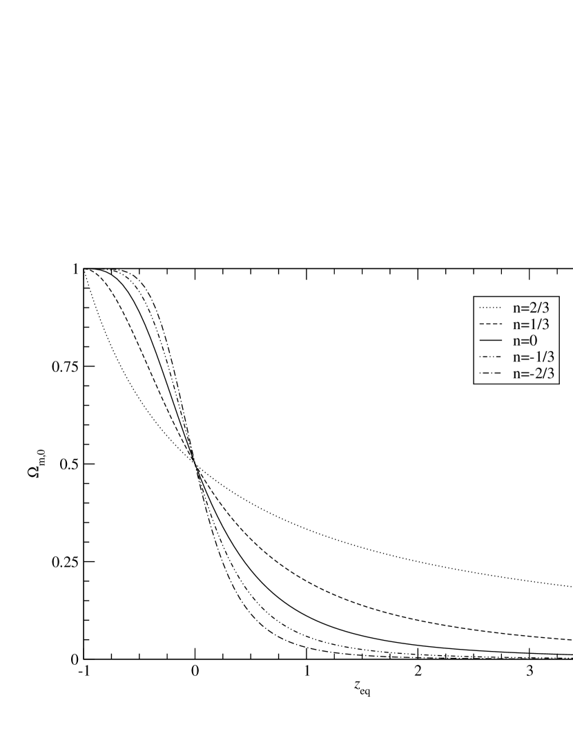
Figure 8: Relation between $\Omega_{\mathrm{m},0}$ and $z_{\mathrm{eq}}$ for different $n$.

Assuming the curvature term $\Omega_{k,0}$ in the Cardassian model we obtained its statistical estimation to be close to zero. In this natural way we got that a nearly flat universe is preferred. Moreover, in this case for Perlmutter sample C the preferred value of $\Omega_{\mathrm{m},0}$ is $0.29$ that is in agreement with CMBR and extragalactic data. While for sample A we got that a universe with higher matter content is preferred.

Let us note that Riess et al. (1998); Perlmutter et al. (1999) obtained the high negative value of $\Omega_{k,0}$ as the best fit, although zero value of $\Omega_{k,0}$ is statistically admissible. To find the curvature they additionally used the data from CMBR and extragalactic astronomy. But in the Cardassian model in natural way the nearly flat universe is favored.

If the flat universe is assumed, in the analysis of the Cardassian universe with sample C we got low but positive values of $n$ and matter density higher than $0.3$. For all other samples we obtained negative values of $n$ (it would also indicate the phamtom fluid with super negative pressure). In turn, when $\Omega_{\mathrm{m},0}$ is fixed to be $0.3$, then $n\approx 0$ is favored.

In general, the results obtained using the Perlmutter and Knop samples are not significantly different. The main advantage of using the Knop sample is the lower errors of estimated parameters in the model. The Tonry sample also gave the results similar to the Perlmutter sample. It can be noted that the Tonry sample does not improve the estimation errors compared with the Perlmutter sample.

From the statistical analysis we found that the Perlmutter and Cardassian models are indistinguishable. Hence, using the philosophy of Occam’s razor the Cardassian model should be rejected if we base on current SN Ia data. However, the Cardassian model has its own advantages and fits well to the present observational data. And till we have no more precise data we should wait before we reject this model.

References

- Freese and Lewis (2002) K. Freese and M. Lewis, Phys. Lett. B 540, 1 (2002), eprint astro-ph/0201229.
- Zhu and Fujimoto (2003) Z.-H. Zhu and M.-K. Fujimoto, Astrophys. J. 585, 52 (2003), eprint astro-ph/0303021.
- Sen and Sen (2003) S. Sen and A. A. Sen, Astrophys. J. 588, 1 (2003), eprint astro-ph/0211634.
- Dev et al. (2003) A. Dev, J. S. Alcaniz, and D. Jain (2003), eprint astro-ph/0305068.
- Perlmutter et al. (1999) S. Perlmutter et al., Astrophys. J. 517, 565 (1999), eprint astro-ph/9812133.
- Knop et al. (2003) R. A. Knop et al. (2003), eprint astro-ph/0309368.
- Tonry et al. (2003) J. L. Tonry et al., Astrophys. J. 594, 1 (2003), eprint astro-ph/0305008.
- Frith (2003) W. J. Frith (2003), eprint astro-ph/031121.
- Weinberg (1972) S. Weinberg, Gravitation and Cosmology (Wiley, New York, 1972).
- Riess et al. (1998) A. G. Riess et al., Astron. J. 116, 1009 (1998), eprint astro-ph/9805201.
- Peebles and Ratra (2003) P. J. E. Peebles and B. Ratra, Rev. Mod. Phys. 75, 559 (2003), eprint astro-ph/0207347.
- Lahav (2002) O. Lahav (2002), eprint astro-ph/0208297.
- Williams et al. (2003) B. F. Williams et al. (2003), eprint astro-ph/0310432.