Wide band X-ray and optical observations of the BL Lac object 1ES 1959+650 in high state

The blazar 1ES 1959+650 was observed twice by BeppoSAX in September 2001 simultaneously with optical observations. We report here the X-ray data together with the optical, $R_{C}$ magnitude, light curve since August 1995. The BeppoSAX observations were triggered by an active X-ray status of the source. The X-ray spectra are brighter than the previously published X-ray observations, although the source was in an even higher state a few months later, as monitored by the ASM onboard RossiXTE, when it was also detected to flare in the TeV band. Our X-ray spectra are well represented by a continuosly curved model up to 45 keV and are interpreted as synchrotron emission, with the peak moving to higher energies. This is also confirmed by the slope of the X-ray spectrum which is harder than in previous observations. Based on our optical and X-ray data, the synchrotron peak turns out to be in the range 0.1-0.7 keV. We compare our data with non simultaneous radio to TeV data and model the spectral energy distribution with a homogeneous, one-zone synchrotron inverse Compton model. We derive physical parameters that are typical of low power High Energy peaked Blazar, characterised by a relatively large beaming factor, low luminosity and absence of external seed photons.

1 Introduction

Blazars constitute the most extreme class of active galactic nuclei: they are radio loud AGN characterized by high luminosity, with rapid and high amplitude variability. They are usually divided into Flat Spectrum Radio Quasars and BL Lac objects, according to the presence or not of broad spectral features. Another blazar distinguishing property is the spectral energy distribution which is marked by two broad peaks (von Montigny et al. 1995): the first, extending from the radio to the UV/X–ray band is usually interpreted as synchrotron emission, while the second, which reaches the $\gamma$–ray band (sometimes TeV frequencies) is explained as an inverse Compton component. Based on this, BL Lacs are further split into two subclasses distinguished by the synchrotron peak frequency: LBL and HBL, Low and High Energy peaked BL Lacs, respectively (Padovani & Giommi 1995). Various models have been proposed to explain the, still debated, origin of the comptonized photons: they could be the synchrotron photons themselves (Maraschi, Ghisellini & Celotti 1992), maybe partly reprocessed by the broad line region (Ghisellini & Madau 1996) or external ambient photons emitted by the accretion disk (Dermer & Shlickeiser 1993) possibly reprocessed to some extent by the broad line region (Sikora, Begelmann & Rees 1994) or by a dusty torus (Blażejowski et al. 2000).

A wide spectral coverage is therefore necessary to understand the physics of these objects: accurate simultaneous multiwavelength spectra and light curves allow us to constrain the mechanism at work and the geometry of the emitting region. HBL in particular have gained much attention in the last decade since many of them have proved to be TeV emitters: the strongest ones are the thoroughly investigated Mkn 421 (Punch et al. 1992) and Mkn 501 (Quinn et al. 1996). Another three sources have then been detected by ground–based Cherenkov telescopes: 1ES 2344+514 (Catanese et al. 1998), PKS 2155-304 (Chadwick et al. 1999) and H 1426+428 (Horan et al. 2002). On the basis of X–ray and radio data, Costamante & Ghisellini (2002) selected a catalogue of BL Lac objects which are most likely to be TeV emitters. One of the most promising objects in this catalogue is 1ES 1959+650, as suggested also by Stecker et al. (1996). Indeed, this source has now been detected in the TeV band (see below).

1ES 1959+650 was discovered in the radio band as part of a 4.85 GHz survey performed with the 91 m NRAO Green Bank telescope (Gregory & Condon 1991; Becker, White & Edwards 1991). Subsequently the source was observed also in the optical band where it displayed large and fast flux variations (e.g. Villata et al. 2000). It shows a complex structure composed by an elliptical galaxy (M${}_{R}=-23$) plus a disc and an absorption dust lane (Heidt et al. 1999). Its redshift ($z$=0.048) was derived by Perlman et al. (1996) from a spectrum obtained at the 2.1 m telescope at Kitt Peak.

The first X-ray measurement of 1959+650 was performed by Einstein-IPC during the Slew Survey (Elvis et al. 1992). Subsequently, the source was observed by ROSAT in 1996, by BeppoSAX in 1997 (Beckmann 2000; Beckmann et al. 2002) and finally by USA and RXTE during 2000 (Giebels et al. 2002). On the basis of a X-ray/radio versus X-ray/optical color–color diagram the source was classified as a BL Lac object by Schachter et al. (1993). According to the new schemes, the source belongs to the HBL class.

In the $\gamma$–ray band, it was observed in 1995 by EGRET on board the CGRO and by the Whipple observatory, but the source was not detected and only upper limits could be set (Weekes et al. 1996); subsequent EGRET observations allowed Hartmann et al. (1999) to put it in the third EGRET catalog, with an average flux of $1.8\times 10^{-7}$ photons cm^-2 s^-1 at energies above 100 MeV.

During the spring and the summer of 1998, it was observed intensively with the Utah Seven Telescope Array detector which recorded a 3.9$\sigma$ total significance above 600 GeV. However, during two epochs, the source was seen above 5$\sigma$ significance (Nishiyama et al. 1999). These data have been confirmed by the HEGRA and the Whipple teams. After 94 hours on–source collected in 2000 and 2001, the HEGRA team detected the source at $8\%$ of the Crab flux with a 5.4 $\sigma$ significance, while from May to July 2002 the source was detected in a much brighter state, up to and above the Crab flux (Horns et al. 2002, Aharonian et al. 2003). Also the Whipple team observed the source for $\sim 39$ hours between May and July 2002, reporting a mean flux of $0.64\pm 0.03$ Crab above 600 GeV, with a significance of 20 $\sigma$ (Holder et al. 2003a,b). Thus, during the May-July 2002 HEGRA and Whipple observations, 1ES 1959+650 was one of the strongest TeV sources in the sky.

1ES 1959+650 is therefore one of the most interesting and frequently observed sources of recent years. In this paper we present two BeppoSAX ToO observations as part of a project for observing active state blazars as detected in optical, X–ray or TeV bands. In particular, these observations were triggered by the active X-ray state of 1ES 1959+650 as observed by the RossiXTE All Sky Monitor (ASM) and are the final observations of this successful BeppoSAX project.

2 Observations and data reduction

The Italian-Dutch satellite BeppoSAX has proved particularly useful for studying blazars because of its extremely large spectral range (0.1-200 keV) which allowed the detection of the transition between synchrotron and Compton emission (Tagliaferri et al. 2000; Giommi et al. 2000; Ravasio et al. 2002) and the interesting comparison of simultaneous soft–X versus hard–X behaviour (Fossati et al. 2000a; Zhang et al. 2002).

For a detailed description of the mission we refer to Boella et al. (1997 and references therein). In our work we have analyzed the data of different co-aligned Narrow Field Instruments aboard the satellite: the Low Energy Concentrator Spectrometer (LECS; 0.1-10 keV), the two (originally three) identical Medium Energy Concentrator Spectrometers (MECS; 1.5-10 keV) still operating and the passively collimated Phoswich Detector System (PDS; 13-300 keV).

Since 1ES 1959+650 was observed to be in a high X-ray state by the RossiXTE-ASM during september 2001, we triggered a BeppoSAX ToO observation, scheduled to last $5\times 10^{4}$ sec. However, because of technical problems, it was stopped after $\sim 5\times 10^{3}$ s. Thus, we were given a second opportunity and some days later a new pointing was performed. In Table 1 we show the log of BeppoSAX observations, together with exposures and count rates for each instrument.

We based our analysis on linearized and cleaned event files available from the online archive of the BeppoSAX Science Data Center (Giommi & Fiore 1998): the events from the two operating MECS are merged together to improve the photon statistic. Using XSELECT V2.0, we extracted light curves and spectra from the event files selecting circular regions centered on the source of 8 and 4 arcmin radii for LECS and MECS respectively, as suggested in Fiore et al. (1999). We also extracted events from off–source regions to test the background stability. For the spectral analysis we preferred to use background files accumulated from long blank field exposures and available from the SDC public ftp site: this choice is motivated by the non uniformity of LECS and MECS backgrounds across the detectors (Fiore et al. 1999; Parmar et al. 1999). In this way the source and background spectra are extracted from the same detector area. For the spectral and temporal analysis we used XSPEC 11.0.1 and XRONOS 5.18 packages, respectively.

	LECS		MECS		PDS
Date	exposure	count ratea	exposure	count rateb	exposure	count ratec
	(s)		(s)		(s)
25 September 2001	$5.8\times 10^{3}$	$1.12\pm 0.015$	$7.2\times 10^{3}$	$1.43\pm 0.016$	$2.97\times 10^{3}$	$0.23\pm 0.099$
28-29 September 2001	$2.6\times 10^{4}$	$1.23\pm 0.008$	$4.8\times 10^{4}$	$1.75\pm 0.007$	$2.3\times 10^{4}$	$0.35\pm 0.036$

Table 1: Log of BeppoSAX observations. ^a 0.1–10 keV; ^b 1.5–10 keV; ^c 15–100 keV.

3 Spectral analysis

In order to reproduce the whole X–ray spectrum we fitted the data of the LECS, MECS and PDS together: to account for the uncertainties in the intercalibration of the instruments it is necessary to use constant rescaling factors. The LECS/MECS normalization acceptable range is [0.67-1], while the PDS/MECS one is [0.77-0.93] (Fiore et al. 1999). In order to reduce the number of fitting parameters and to be consistent with previous work, we fixed them at 0.72 and 0.9, respectively.

3.1 25 September 2001

Although the first observation was very short the source was detected even by the PDS up to 35 keV: the good channels were then grouped in 3 bins. We first analyzed LECS + MECS spectra and then we added the PDS data: since for this observation and for that of the 28-29 September, the addition of PDS data does not change significantly the best fit parameters, in our discussion we will always refer to the analysis performed on the full set of LECS–MECS–PDS spectra.

We fitted the data with a power–law or a broken power–law model, first fixing the absorption parameter N_H to the Galactic value (N${}_{\rm H}=1.0\times 10^{21}$ cm^-2 as determined from 21 cm measurements by Dickey & Lockman (1990)) and then leaving it free: the best fit parameters of each model are given in Table 2 together with the flux at 1 keV and the integrated [2-10] keV flux. Using the Galactic absorption value we always obtained bad fits: large negative residuals toward low frequencies are evident. With the N_H free to vary, instead, we obtained good fits to the spectrum both with a simple power–law ( energy index $\alpha=1.45\pm 0.05$, N${}_{\rm H}=2.1\times 10^{21}$ cm^-2; $\chi^{2}_{r}/d.o.f.=0.7/32$) and a steepening broken power–law model (N${}_{\rm H}=1.8\times 10^{21}$ cm^-2; $\chi^{2}_{r}/d.o.f.=0.6/30$). The best–fit parameters of the broken power–law model are $\alpha_{1}=1.3\pm 0.1$ and $\alpha_{2}=1.5\pm 0.1$ with the break located at 2.7 keV. The $\chi^{2}$ values do not allow us to distinguish between these spectral models which are both acceptable. Note, however, that in both cases the resulting N_H values are significantly higher than the Galactic value.

These results are consistent with previous X–ray observations of the source. Beckmann et al. (2002) analyzed the 1997 BeppoSAX and the ROSAT All Sky Survey data finding a N_H value in excess of the Galactic value: more precisely, using a power–law model they found N${}_{\rm H}=2.55\times 10^{21}$ cm^-2 for the BeppoSAX spectrum and N${}_{\rm H}=1.6\times 10^{21}$ cm^-2 for the ROSAT spectrum. For the BeppoSAX observation they also fitted a broken power–law model finding an intermediate value. This extra absorption required to fit the X-ray data could be due either to a real intrinsic absorption at the source or to an artifact due to a progressive steepening of the spectrum that can not be reproduced by a simple power–law or broken power–law model. The assumption of an absorption higher than the Galactic value would not be necessary if a model which can intrinsically account for a progressive steepening of the spectrum is used. Therefore, we tried to reproduce the BeppoSAX spectrum with the continuously curved model described in Fossati et al. (2000b):

$$F(E)=KE^{-\alpha_{-\infty}}\big{[}1+\big{(}\frac{E}{E_{B}}\big{)}^{f}\big{]}^{(\alpha_{-\infty}-\alpha_{+\infty})/f}$$ (1)

where $\alpha_{-\infty}$ and $\alpha_{+\infty}$ are the asymptotic values of the energy indices, while $E_{B}$ and $f$ are the parameters that determine the spectral bending. We applied this model to the whole LECS–MECS–PDS spectrum fixing the absorption parameter to the Galactic value. First we found the value of the parameter $f$ that minimizes the $\chi^{2}$ when all the other parameters are left free to vary obtainiong $f=1.1$. Then, we repeated the fitting a few times to derive the spectral indices at several reference energies (0.5, 1, 10, 35 keV), checking that each time the same values for the varying parameters were obtained (see Fossati et al. 2000b for more details of this procedure). The data are well fitted, with only the Galactic absorption, ($\chi^{2}_{r}/d.o.f.=0.6/31$) by a curve which is flat below 1 keV and steepens toward higher energies; the model reaches a slope $\alpha=1$ at $1.2\pm 0.1$ keV. In Table 3 we give the best–fit parameters of the model.

A possible inconvenience of this model is that it is so flexible to adjust the parameters for a wide rage of spectral curvatures and then it results poorly sensitive to the actual N_H value. Therefore, we also considered another curved model using a logarithmic parabola, which provides a reasonable representation of the wide band spectral distribution for the synchrotron component of blazars:

$$F(E)=K\leavevmode\nobreak\ (E/E_{1})^{-(a+b\leavevmode\nobreak\ Log(E/E_{1}))}\leavevmode\nobreak\ \leavevmode\nobreak\ \leavevmode\nobreak\ .$$ (2)

This model has recently been used to fit the optical-X-ray spectra of various objects (Giommi et al. 2002; Massaro et al. 2003a,b). In our computations we fixed the $E_{1}$ value at 1 keV. With the N_H fixed to the Galactic value, this model provides a good fit to the data although not as good as the previous curved model. A lower $\chi^{2}$ is obtained if we leave the N_H free to vary, the resulting best–fit value is very similar to the one obtained with the broken power–law model. A summary of the best–fit parameters is given in Table 3 .

       

Figure 1: 1ES 1959+650 BeppoSAX spectrum of 28-29 september 2001. Left panel: LECS + MECS + PDS spectrum fitted with a power–law plus intrinsic absorption model: positive residuals are evident below 0.8 keV, while there are negative residuals in the PDS range. Right panel: LECS + MECS + PDS spectrum fitted with a broken power–law plus intrinsic absorption model provides a better fit, although the PDS data still lie below the model.

3.2 28-29 September 2001

The second pointing had an exposure about a factor of 6 longer than the previous one. Furthermore 1ES 1959+650 was $\sim$20% brighter than in the first observation (see Table 1). We therefore had data with much higher counts, useful for a more accurate investigation of the spectral shape. The PDS was able to detect the source up to slightly higher frequencies ($\sim 45$ keV) than the previous observation. We again grouped the PDS data in 3 bins. Also in this case we will refer to the analysis performed on LECS+MECS+PDS data as a whole, repeating the fitting process with the absorption parameter fixed to the Galactic value or free to vary. Spectral fits using power–law or broken power–law models with the Galactic N_H are not acceptable because of the rather high $\chi^{2}$ values (see Table 2). With a free N_H we again find values that exceed the galactic value and are consistent with those of the September 25 observation and of Beckmann et al. (2002). However, in this case the BeppoSAX spectrum is also badly fitted by a single power–law model ($\chi^{2}_{r}$/d.o.f.=2.3/32) with the N_H free to vary. As can be clearly seen in Fig. 1, this model leaves positive residuals toward low energies and negative ones in the PDS range: the spectrum seems to be continuously steepening. Leaving the absorption parameter free, a broken power–law model with a break at E${}_{b}\sim 2.6$ keV ($\Delta\alpha\sim 0.26$) provides a better representation to the data ($\chi^{2}_{r}$/d.o.f.=1.0/30), although the negative residuals at higher energies are still not completely removed (Fig. 1). Similarly to what was obtained in the analysis of the previous observation, to fit BeppoSAX data with a broken power–law model we need a column density higher than the Galactic value. We then fitted our data using the curved model of Fossati et al. (2000b). The data are well fitted with a curvature parameter $f=1.25$ and a fixed Galactic absorption value ($\chi^{2}_{r}/d.o.f.=1.1/31$). In this case the negative residuals left in the PDS range by the broken power–law model disappear (see Fig. 2). Best-fit parameters are given in Table 3. Similarly to what was observed some days before, the model is hard below 1 keV and steepens toward higher energies up to $\alpha_{45keV}=1.48$; the turning point where the model reaches $\alpha=1$ is shifted to a slightly larger frequency ($1.55\pm 0.05$ keV). Finally, we applied the parabolic model, but this time a good fit could be obtained only with the N_H free to vary, finding an absorption value similar to that obtained with the broken power–law model (see Table 3).

To summarize our results, on September 2001, 1ES 1959+650 X–ray spectra were convex and could be fitted either with a steepening broken power–law or a parabolic model with an interstellar absorption exceeding the Galactic value. Taking into account that optical images of the host galaxy (see Sect. 5) show that it is crossed by a strong dust lane, it is well possible that this additional N_H is due to some contribution within the host galaxy. The higher value of N_H derived from the X-ray data is in line with the E(B-V) values derived from optical observations (see section 5). The only model that fits the data with the N_H value fixed at the Galactic value is the curved model proposed by Fossati et al. (2000b). However, the X-ray spectral shape that one derives in this case is not very plausible in the overall SED of the source, with a synchrotron peak above 1 keV. Thus, we think that this representation, with the N_H fixed at the Galactic value, is not realistic. To conclude, our X-ray data imply an absorption higher than the Galactic value and a peak of the X-ray emission in the 0.1-0.7 keV range.

Figure 2: 1ES 1959+650 BeppoSAX spectrum of 28-29 september 2001: LECS + MECS + PDS spectrum fitted with the curved model. The negative residuals left by simple and broken power–law models in PDS range disappear.

model	NH	$\alpha_{1}$	Eb	$\alpha_{2}$	F1keV	F${}^{*}_{2-10keV}$	$\chi 2_{r}$/d.o.f.
	($\times 10^{22}$ cm-2)		keV		($\mu$Jy)
25 September 2001
LECS + MECS + PDS
power–law	0.1	1.25			31.3	8.6	4.95/33
power–law	$0.21\pm 0.03$	$1.45\pm 0.05$			40.3	8.3	0.70/32
broken power–law	0.1	$0.9^{+0.1}_{-0.5}$	$1.9^{+0.5}_{-0.7}$	$1.45\pm 0.1$	29.5	8.3	1.20/31
broken power–law	$0.18\pm 0.03$	$1.3\pm 0.1$	$2.7^{+1.2}_{-0.8}$	$1.5\pm 0.1$	37.2	8.3	0.55/30
28-29 September 2001
LECS + MECS + PDS
power–law	0.1	1.15			33.5	10.6	24/33
power–law	$0.22$	$1.3$			42.1	10.4	2.3/32
broken power–law	0.1	0.85	2.1	1.3	30.5	10.4	2.8/31
broken power–law	$0.16^{-0.03}_{+0.02}$	$1.1\pm 0.1$	$2.6^{+0.5}_{-0.4}$	$1.36^{+0.03}_{-0.04}$	37.0	10.4	1.0/30

Table 2: Best fit model parameters. ^∗ F_2-10keV flux in unit of $10^{-11}$ erg cm^-2 s^-1.

LECS + MECS + PDS: curved model
25 September 2001
$\alpha_{0.5keV}$	$\alpha_{1keV}$	$\alpha_{10keV}$	$\alpha_{35keV}$	F${}^{*}_{0.5-2keV}$	F${}^{*}_{2-10keV}$	$\chi^{2}_{r}$/d.o.f
$0.0^{+0.4}_{-0.1}$	$0.9\pm 0.1$	$1.55^{+0.1}_{-0.05}$	$1.6^{+0.1}_{-0.05}$	7.5	8.3	0.6/31
28-29 September 2001
$0.2\pm 0.2$	$0.74\pm 0.03$	$1.43\pm 0.03$	$1.48^{+0.05}_{-0.04}$	7.8	10.4	1.1/31
LECS + MECS + PDS: parabolic model
25 September 2001
NH	$a$	$b$	F1keV	F${}^{*}_{0.5-2keV}$
	F${}^{*}_{2-10keV}$	$\chi^{2}_{r}/d.o.f.$
($10^{22}$ cm-2)			($\mu$Jy)
$0.17\pm 0.06$	$1.24\pm 0.27$	$0.18\pm 0.25$	36.9	7.49	8.26	0.63/31
FIXED	$1.925\pm 0.075$	$0.465\pm 0.1$	30.5	7.43	8.22	0.96/32
28-29 September 2001
$0.16\pm 0.03$	$1.06\pm 0.10$	$0.21\pm 0.09$	37.0	7.82	10.4	1.18/31
FIXED	1.83	0.4	31.7	7.82	10.4	2.4/32

Table 3: Best fit parameters for the curved and parabolic models of LECS–MECS–PDS spectrum. ^∗ fluxes are in units of $10^{-11}$ erg cm^-2 s^-1. For the curved model, the absorption parameter is fixed to the Galactic value of N${}_{\rm H}=1.0\times 10^{21}$ cm^-2; while the best–fit curvature parameters are $f=1.1$ and $f=1.25$ for the first and the second observation, respectively, reaching a slope $\alpha=1$ at $1.2\pm 0.1$ and $1.55\pm 0.05$ keV for the two spectra.

3.3 Archival X-ray data

It is interesting to compare the 2001 BeppoSAX spectra to those previously measured by other X–ray missions: Einstein, ROSAT (1996), BeppoSAX itself (1997), RXTE and USA (2000). The results of these observations are summarised in Table 4. During Einstein, ROSAT and the 1997 BeppoSAX observations, the source had a flux of F${}_{2-10keV}\sim 10^{-11}$ erg cm^-2 s^-1. In particular, Einstein measured a 2 keV flux which was $\sim 40\%$ and $\sim 60\%$ higher than the 1997 BeppoSAX and 1996 ROSAT measurements, respectively. 1ES 1959+650 was monitored by RXTE and by USA through the summer and the autumn of 2000. The source was in a higher state (F${}_{2-10keV}\sim 10^{-10}$ erg cm^-2 s^-1), with a flare reaching a 2-10 keV flux of $2.3\times 10^{-10}\ {\rm erg\ cm^{-2}\ s^{-1}}$ (14 November 2000, USA; Giebels et al. 2002). The source was in a high state also during our observations, similar to those measured by RXTE and a little fainter than the flare of November 2000, monitored by USA.

These X–ray spectra are always soft ($\alpha>1$) and can be explained as synchrotron emission. The BeppoSAX spectra of 2001 are the hardest measured so far (below 3 keV), as if the synchrotron component were peaking at higher energies with respect to the other historical observations (see Discussion).

Instrument	Date	$\alpha$	F2-10keV
			($10^{-11}$ erg cm-2 s-1)
ROSAT	31 March 1996	$1.76^{+0.44}_{-0.21}$	1.04
BeppoSAX	4 May 1997	$1.64\pm 0.08$	1.29
RXTE	July–September 2000	1.38–1.68	8.4–14
USA	October–November 2000		4.87–22.6
BeppoSAX	25 September 2001	1.31a	8.29
BeppoSAX	28-29 September 2001	1.12a	10.42

Table 4: Historical X–ray observations of 1ES 1959+650. ^a soft X–ray spectral index.

4 Temporal analysis

We examined the observation of September 25 for short time variability, rebinning the light curves with a resolution of 600 seconds and selecting only bin intervals with an effective exposure greater than $20\%$ (i.e. all bins that have data for less than 20bin are rejected). Because the spectrum seems to steepen at $\sim 3$ keV, we analysed the LECS and MECS light curves in two different energy ranges: [0.3-3] keV LECS and [3-10] keV MECS bands. During this short period, the observation was interrupted after $\sim 7000$ s, the source seemed to be quiet: both LECS [0.3-3] keV and MECS [3-10] keV light curves are well fitted by a constant model, with a maximum allowed variability lower than 20%.

The second observation is longer ($\sim 5\times 10^{4}$ sec) and can give us more information. During this run 1ES 1959+650 was still displaying a convex spectrum in the LECS-MECS range, with a break at $\sim 2.5$ keV and a further steepening in the PDS range. Therefore we again split our field of analysis extracting [0.15–2.5] keV LECS and [2.5–10] keV MECS light curves, together with a PDS curve in the range [15-45] keV (Fig. 3). For the LECS and MECS data we chose a binning time of 1000 seconds, while for the PDS we rebinned the data in 3600 second intervals, due to lower statistic. In each curve we accepted only bins with at least $20\%$ of effective exposure time. Also during this observation BeppoSAX did not detect very large variability, with a possible indication of larger variability above the break. In fact, we get a high probability that the source is constant below the break for the LECS data, while MECS [2.5-10 keV] and PDS light curves are badly fitted by a constant model (constancy probability $<1\%$). This is not surprising since we are observing a steepening synchrotron spectra: a little hardening of the synchrotron component will cause small flux variations in the proximity of the peak but larger flux variations as the spectrum steepens at higher energies. In any case these variations are small and the main conclusion of this analysis is that the source did not clearly show brightness changes during the two BeppoSAX observations. Given that the source flux in the second observation increased by only $\sim$20% it is likely that it remained approximately stable at this high level at least from September 25 up to September 29.

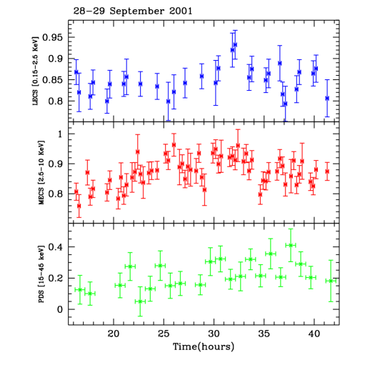
Figure 3: 1ES 1959+650 28-29 September 2001 light curves. Top panel: [0.15-2.5] keV LECS $1000\,s$ binned light curve. Mid panel: [2.5-10] keV MECS $1000\,s$ light curve. Bottom panel:[15-45] keV PDS $3600\,s$ binned light curve.

5 Optical observations

Figure 4: The optical, $R_{C}$ magnitude, light curve of 1ES 1959+650 since August 1995. Open triangles are data from the Perugia observations, filled circles are from Roma-Vallinfreda. The vertical line indicates the dates of the BeppoSAX pointings, activated by an X-Ray trigger.

We observed 1ES 1959+650 for about nine hours in the Cousins R band during the night of September 28-29 2001 with the 50 cm f/4.5 Newtonian reflector of the Astronomical Station of Vallinfreda (Rome) (e.g. Maesano et al. 1997). The reference photometric sequence by Villata et al. (1998) was used, except for their star 5, which is variable as already pointed out by Nikolashvili, Kurtanidze and Richter (1999). The source remained constant around a mean value of R=14.67 within our sensitivity of 0.02 mag (Maesano et al. 2002).

To measure properly the optical SED of a blazar it is necessary to subtract from the observed flux values the contribution of the underlying host galaxy. In the case of 1ES1959+65 the host is detectable even with the short focal length of our 50 cm telescope. Heidt et al. (1999) using the 2.5m NOT telescope at La Palma found that a De Vaucoulers profile ($r_{e}=9.5^{\prime\prime}$, R_tot=14.80) does not give an acceptable $\chi^{2}$ for the fit to the surface brightness of this galaxy, at variance with other host galaxies of their sample of BL Lacs. They found a better agreement using a different exponent (0.41 instead of 0.25), with an effective radius $r_{e}$=10.3^′′, a small additional disk component, with $r_{e}$=4.8^′′ and a total galaxy R magnitude R_tot=14.9. Furthermore they found a dust lane 1^′′ north of the nucleus. Scarpa et al. (1999) using HST images confirmed the presence of the dust lane but found a satisfactory fit to the brightness profile with a De Vaucouleurs law ($r_{e}$=5.1^′′, R_tot=14.92) without the need for an additional disk. We remark however that the derived contribution of the host galaxy depends on the seeing conditions: a larger seeing spreads the galaxy image over a larger apparent radius, so that the galaxy appears fainter within a given radius. This effect is stronger if the intrinsic $r_{e}$ is smaller than the seeing radius, which is not our case, however, whichever estimate of $r_{e}$ (4.8 or 9.5 arcsec) is assumed.

For the purpose of this paper, i.e. to evaluate the contribution of the host galaxy within our photometric radius, we compute the R magnitude integrating a De Vaucouleurs profile for both estimates, finding R=15.66 following Scarpa et al. (1999) and R=15.95 following Heidt et al. (1999) (see Table 5). Both values are fainter than the minimum recorded luminosity of the source, as can be derived from the historical light curve shown in Fig. 4, built using the data obtained in the course of a monitoring program of a sample of bright blazars carried out since 1994 by the Roma and Perugia groups. The telescopes used were the AIT (0.40 m) of the Perugia Observatory (Tosti et al. 1996) and the reflector telescope of Vallinfreda. The source shows a flux variability between R=14.4 and R=15.2, without evident periodicity. Some additional photometric points have been published by Villata et al. (1998), also giving the source luminosity within the above quoted range.

After subtraction of the galaxy contribution we computed the intrinsic flux of the source (in mJy) adopting the extinction curve by Rieke and Lebofsky (1985) and two possible values for the colour excess: E(B$-$V)=0.16 (consistent with the Galactic value for the N_H, implying A_R=0.43) and E(B$-$V)=0.26, consistent with the N_H value derived from the X-ray data. The zero magnitude flux value (3.12 Jy at R=0.0) is taken from Elvis et al. (1994) (see Table 5).

Mag	Tot. mag	galaxy	Tot	gal	net	Extin. corr.	Intrin.	Extin. corr.	Intrin.
band	value	contr.	mJy	mJy	mJy	E(B-V)=0.16	mJy	E(B-V)=0.26	mJy
R	14.65	15.66	4.30	1.70	2.60	1.48	3.86	1.84	4.78
R	14.65	15.95	4.30	1.30	3.00	1.48	4.46	1.84	5.52
V	15.11	16.43	3.19	0.94	2.25	1.59	3.58	2.12	4.77
V	15.11	16.72	3.19	0.72	2.47	1.59	3.93	2.12	5.23

Table 5: Observed total (blazar+galaxy) R magnitude and derived intrinsic values for the blazar nucleus. The contribution of the galaxy is calculated assuming two different profiles (see text). The V magnitude has not been observed, but it is derived thanks to a very constant V-R value observed over the years for this source, see text.

The V$-$R colour index of the source is remarkably constant in our database, 0.46, with a dispersion of 0.01. Thus, assuming an intrinsic value of B$-$V=0.61 for the host galaxy (observed B$-$V=0.77) following Fukugita et al. (1995), we can derive the V mag (see Table 5) and a spectral energy slope value, in the Log($\nu$)–Log(F_ν) plane, of 0.49 and 0.83 for the two estimates of the host galaxy magnitude, respectively.

6 The Spectral Energy Distribution

We have constructed the SED of 1ES 1959+650 (shown in Fig. 5) using our BeppoSAX and optical data (filled symbols) and data from the literature. We also include the previous X-ray spectra measured by ROSAT and BeppoSAX (from Beckmann et al 2002).The TeV spectrum measured during a large flare in May 2002 has been recently reported by Aharonian et al. (2003). The same paper gives the TeV flux observed for the period 2000-2001. In the SED we assumed that the TeV spectral shape remains almost unchanged with flux and simply rescaled the spectrum to the average flux observed during 2000-2001.

The spectral data presented in the previous sections show that the X–ray spectral distribution of 1ES 1959+650 is characterised by a well defined curvature. In the case of the parabolic model, a measure of this curvature is given by the parameter $b$ in Eq.(2). It is interesting to compare this result with those of Mkn 421, whose BeppoSAX data have been analysed with the same spectral law (Massaro et al. 2003b). The typical $b$ values for this source are higher than 0.3 and only during the bright phase of spring 2000 are close to 0.2, a value comparable to that measured in the September 28-29 observation of 1ES 1959+650 and equal to 0.21. If the spectral and luminosity trends of the sources are similar this may be an indication that in the previous observations, when it was much fainter (see Table 4), the spectral curvature could have been greater as also indicated by the steeper spectral slopes. Furthermore, with this model one can easily derive the energy of the maximum in the SED (see Massaro et al. 2003b for details) which is $\sim$0.1 and $\sim$0.7 keV in the two observations, respectively. Similar values are found in the intermediate luminosity states of Mkn 421, while during flares the peak ranges between 2.5 and 5 keV. We can therefore conclude that the typical peak energies for 1ES 1959+650 are around $\sim$0.1–0.3 keV, approaching 1 keV in the X-ray high states.

We have used a homogeneous, one–zone synchrotron inverse Compton model to reproduce the SEDs of 1ES 1959+650. The model is very similar to the one described in detail in Spada et al. (2001), it is the “one–zone” version of it. The same model was applied to S5 0716+714 and OQ 530 by Tagliaferri et al. (2003); further details can be found in Ghisellini, Celotti & Costamante (2002), where the same model has been applied to low power BL Lacs. The main assumptions of the model are:

• The source is cylindrical, of radius $R$ and thickness $\Delta R^{\prime}=R/\Gamma$ (in the comoving frame, where $\Gamma$ is the bulk Lorentz factor).

• The source is assumed to emit an intrinsic luminosity $L^{\prime}$ and to be observed at a viewing angle $\theta$ with respect to the jet axis.

• The particle distribution $N(\gamma)$ is assumed to have the slope $n$ [$N(\gamma)\propto\gamma^{-n}$] above the random Lorentz factor $\gamma_{\rm c}$, for which the radiative (synchrotron and inverse Compton) cooling time equals $\Delta R^{\prime}/c$. The motivation behind this choice is the assumption that relativistic particles are injected into the emitting volume for a finite time, which we take roughly equal to the light crossing time of the shell. This crossing time is roughly equal to the time needed for two shells to cross, if they have bulk Lorentz factor differing by a factor around two. The electron distribution is assumed to cut–off abruptly at $\gamma_{\rm max}>\gamma_{\rm c}$. We then assume that between some $\gamma_{\rm min}$ and $\gamma_{\rm c}$ the particle distribution $N(\gamma)\propto\gamma^{-(n-1)}$. This choice corresponds to the case in which the injected particle distribution is a power law ($\propto\gamma^{-(n-1)}$) between $\gamma_{\rm min}$ and $\gamma_{\rm max}$, with $\gamma_{\rm min}<\gamma_{\rm c}$. Below $\gamma_{\rm min}$ we assume $N(\gamma)\propto\gamma^{-1}$. The value of $\gamma_{\rm max}$ is not crucial, due to the fact that the electron distribution, for our sources, is steep. It has been chosen to be a factor $\sim 100$ larger than $\gamma_{\rm min}$.

According to our X–ray data, the peak of the synchrotron spectrum occurs in the 0.1–0.7 keV band. This motivates the choice of the adopted $\nu_{\rm peak}$ as listed in Table 6. This constrains the values of the input parameters of our model. Since we determine $\gamma_{\rm peak}$ as the energy of those electrons that can cool in the injection time (i.e. $\gamma_{\rm peak}=\gamma_{\rm c}$), there is a relation between $\nu_{\rm peak}$ and the cooling rate. If the latter is dominated by synchrotron emission, the location of $\nu_{\rm peak}$ constrains the value of the magnetic field. This in turn fixes the relative amount of inverse Compton radiation.

The remaining degree of freedom for the choice of the input parameters is due to the value of the beaming factor (i.e. $\Gamma$ and the viewing angle $\theta$), and to the redshift. Another important input parameter is the size of the emitting region. Although the source did not show fast variability during our BeppoSAX observations, it is known to be variable, with a minimum observed variability timescale of few hours (e.g. Holder et al. 2003a,b; Aharonian et al. 2003). The size of the emitting region is therefore constrained to be less than one light–day (i.e. $R\leq ct_{\rm var}\delta/(1+z)$). Although a one–zone homogeneous model is forced to use the minimum variability timescale observed at any band to constrain the size, it is also clear that this model is a simplification of a scenario which may be more complex. Our choice of $R=9\times 10^{15}$ cm and $\delta\sim 18$ corresponds to a minimum variability timescale of $t_{var}\sim 5$ hours.

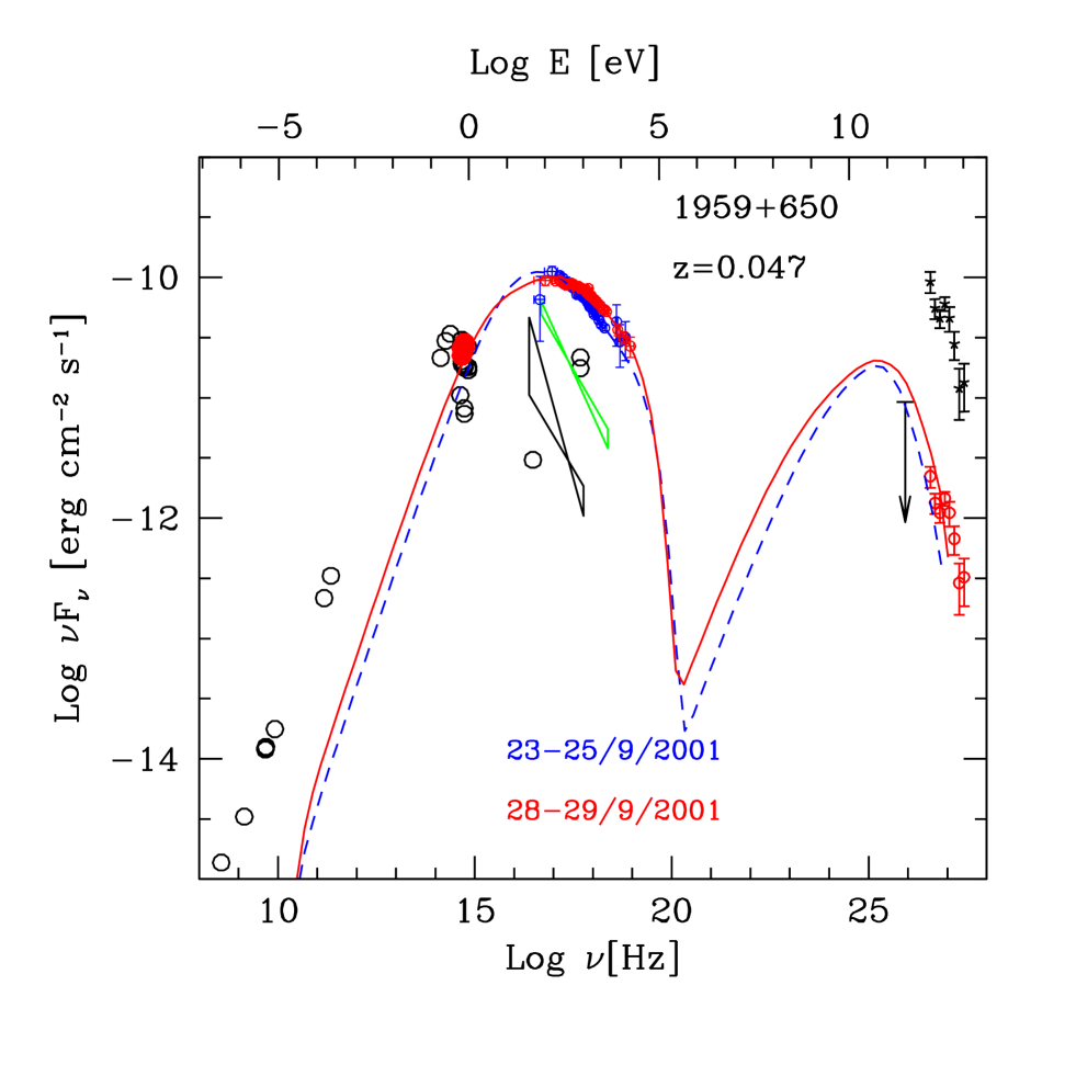
Figure 5: The SED of 1959+650. Non simultaneous data (star symbols) have been collected from the NASA Extragalagtic Database (NED). The “butterflies” in the X-ray region mark the ROSAT (lower) and the previous Beppo (upper) spectra (from Beckmann et al. 2000). The filled circles represent our optical and X-ray data. The lines refer to the SSC models for the two BeppoSAX observations. The TeV data (upper symbols) are from Aharonian et al. (2003) and refer to the flare in May 2002. For the plotted lower TeV data we assume no change in spectrum, and we have simply rescaled the May 2002 data by the amount corresponding to the average flux observed during the years 2000–2001, as reported by Aharonian et al. (2003).

The input parameters are listed in Table 6 and the model fits are shown in Fig. 5. The applied model is aimed at reproducing the spectrum originating in a limited part of the jet, thought to be responsible for most of the emission. This region is necessarily compact, since it must account for the fast variability shown by all blazars, especially at high frequencies. The radio emission from this compact region is strongly self–absorbed, and thus the model cannot account for the observed radio flux. This explains why the radio data are above the model fits in the figure.

Table 6: Model Input Parameters. Column (1): name of the source; column (2): observation date; column (3): intrinsic luminosity $L^{\prime}$; column (4): magnetic field $B$; column (5): size of the emitting region $R$; column (6): bulk Lorentz factor $\Gamma$; column (7): viewing angle $\theta$ (in degrees); column (8): beaming factor $\delta$; column (9): slope of the particle distribution $n$; column (10): minimum Lorentz factor of the injected electrons $\gamma_{\rm min}$; column (11): Lorentz factor of the electron emitting at the peaks, $\gamma_{\rm peak}$; column (12): synchrotron peak frequency $\nu_{\rm peak}$. Note that $\gamma_{\rm peak}$ and $\nu_{\rm peak}$ are derived quantities and not input parameters.

date	$L^{\prime}$	$B$	$R$	$\Gamma$	$\theta$	$\delta$	$n$	$\gamma_{\rm min}$	$\gamma_{\rm peak}$	$\nu_{\rm peak}$
	erg s-1	G	cm							Hz
23 Sep 2001	8.0e40	0.9	9e15	14	3.1	17.8	3.8	1.2e4	4.0e4	9.6e16
29 Sep 2001	9.0e40	0.8	9e15	14	3.1	17.8	3.6	7.0e3	5.0e4	1.3e17

7 Discussion and conclusions

During both BeppoSAX observations, triggered by an active X-ray status of the source, we detected X-ray spectra that steepen with increasing energies, up to 45 keV. The observed spectra are probably due to synchrotron emission, with the synchrotron peak moving to higher energies with respect to previous observations. 1ES 1959+650 belongs to the class of HBL, being characterized by a synchrotron peak in the soft X–ray range. This is confirmed by our BeppoSAX observations, which caught the source in a high X–ray state. The slope of the X–ray spectrum is harder than during previous X–ray observation (see Fig. 5), suggesting a “harder when brighter” behavior, common to many other blazars, at least at frequencies above the synchrotron peak (indications exist that the same behavior is shown also at frequencies above the inverse Compton peak, see e.g. 3C 279, Ballo et al. 2002; PKS 0528+134, Ghisellini et al. 1999).

We do not know yet, however, if 1ES 1959+650, at still higher X–ray (2–10 keV) fluxes, is similar to the flaring state of Mkn 501 (during summer 1997) with a flat ($\alpha_{x}<1$) X–ray spectrum peaking at hundreds of keV, or resembles instead the X-ray spectrum of Mkn 421 which has been always observed with $\alpha_{x}>1$. The physical parameters derived by applying our one–zone SSC model are typical of all low power HBL objects, characterized by a relatively large beaming factor, low luminosity and absence of external seed photons testified also by the very weak (if any) broad emission lines. One can compare the parameters derived in this paper with those derived by a sample of BL Lac objects in Ghisellini, Celotti & Costamante (2002) to see that all sources in this class are characterized by similar parameters. These are the sources which are among the best candidates to be strong TeV emitters (see Costamante & Ghisellini 2002), and in fact 1ES 1959+650 recently has been detected at TeV energies at levels above the Crab by the WHIPPLE and HEGRA Cherenkov telescopes (Holder et al. 2003a, Aharonian et al. 2003). At the time of the TeV flares the X–ray flux was larger than during our BeppoSAX observations, in fact it was in the brightest X-ray state of the source in the last seven years, as monitored by ASM onboard RossiXTE (Holder et al. 2003b). This confirms the strong correlation between X–ray and TeV emission, in turn confirming that the same population of electrons are emitting in both bands. However, one very rapid TeV flare (doubling timescale of 7 hours) was detected by WHIPPLE without a corresponding brightening of the X-ray flux (Holder et al. 2003b). This is clearly difficult to explain with one-zone SSC model. If more examples of this intriguing flare episode will be detected in this and other sources, then some extra complexity in the model will be necessary.

This is the second source in our BeppoSAX ToO program that has been observed because it was in an active X-ray state, the other one being PKS2005-489 (Tagliaferri et al. 2001). In both cases, only the synchrotron component was observed with the synchrotron emission peaking at 1-2 keV and no fast variability was detected. For six other sources the trigger came from the optical band. Thus, we have probably been biased toward sources that have an higher optical variability. These should be the blazars which have the synchrotron peak in the IR-optical band and these are of course essentially LBL or intermediate blazars. For all of them we detected either only the Compton component or both the synchrotron and Compton components (see Tagliaferri et al. 2002). Moreover in three cases we detected very fast variability in the X-ray band, but only for the synchrotron component (ON231: Tagliaferri et al. 2000; BL Lac: Ravasio et al. 2002; S5 0716+714: Tagliaferri et al. 2003). This can be interpreted as the presence in the X–ray band of a Compton component (slowly variable on time scale of months), and the tail of a synchrotron component with fast and the erratic variability.

Thus, we can conclude that, although our sample of BeppoSAX ToO observations is limited, the behaviour of LBL-intermediate blazars in the X-ray band is different than that of HBL, when they are both in a high state of activity.

- (1) Aharonian F., Akhperjanian A., Beilicke M., et al., 2003, submitted to A&AL, astro-ph/0305275
- (2) Ballo L., Maraschi L., Tavecchio F., et al., 2002, ApJ 567, 50
- (3) Becker R.H., White R.L. & Edwards A.L., 1991, ApJS, 75, 1
- (4) Beckmann V., 2000, PhD dissertation, Universität Hamburg
- (5) Beckmann V., Wolter A., Celotti A., Costamante L., Ghisellini G., Maccacaro T. & Tagliaferri G., 2002, A&A, 383, 410
- (6) Blażejowski M., Sikora M., Moderski R. & Madejski G.M., 2000, ApJ, 545, 107
- (7) Boella G., Butler R., Perola G.C. et al., 1997, A&AS, 122, 299
- (8) Catanese M. et al., 1998, ApJ, 501, 616
- (9) Chadwick P.M., 1999, ApJ, 513, 161
- (10) Costamante L. & Ghisellini G., 2002, A&A, 384, 56
- (11) Dermer C. D. & Schlickeiser R., 1993, ApJ, 416, 458
- (12) Dickey J.M. & Lockman F.J., 1990, ARAA, 28, 215
- (13) Elvis M., Plummer D., Schachter J. & Fabbiano G., 1992, ApJS, 80, 257
- (14) Fiore F., Guainazzi M & Grandi P., 1999, Cookbook for NFI BeppoSAX Analysis v.1.2, available at www.asdc.asi.it
- (15) Fossati G., Celotti A., Chiaberge M., Zhang Y.H., Chiappetti L., Ghisellini G., Maraschi L., Tavecchio F., Pian E. & Treves A., 2000a, ApJ 541, 153
- (16) Fossati G., Celotti A., Chiaberge M., Zhang Y.H., Chiappetti L., Ghisellini G., Maraschi L., Tavecchio F., Pian E. & Treves A., 2000b, ApJ, 541, 166
- (17) Fukugita M., Shimasaku K., Ichikawa T., 1995, PASP 107, 945
- (18) Ghisellini G., Celotti A., Costamante L., 2002, A&A, 386, 833
- (19) Ghisellini G., Costamante L., Tagliaferri G., et al., 1999, A&A 348, 63
- (20) Ghisellini G. & Madau P., 1996, MNRAS, 280, 67
- (21) Giebels B., Bloom E.D., Focke W., Godfrey G., Madejski G., Reilly K.T., Parkinson P.M., Shabad G. et al., 2002, ApJ, 571, 763
- (22) Giommi P., Capalbi M., Fiocchi M., Memola E., Perri M., Piranomonte S., Rebecchi S., Massaro E., 2002, in “Blazar Astrophysics with BeppoSAX and other observatories”, eds P.Giommi, E.Massaro, G.Palumbo (ASI Special Publication, printed at ESA-ESRIN)
- (23) Giommi P. & Fiore F., 1998, in:“The 5th International Workshop on Data Analysis in Astronomy”, Erice, Italy, V. Di Gesú, M.J.B. Duff, A. Heck, M.C. Maccarone, L. Scarsi, H.U. Zimmermann (eds.), Word Scient. Publ., p.73
- (24) Gregory P.C. & Condon J.J., 1991, ApJS, 75, 1011
- (25) Hartman R.C. et al., 1999, ApJS, 123, 79
- (26) Heidt J., Nilsson K., Sillapää A., Takalo L.O., Pursimo T., 1999, A&A, 341, 683
- (27) Holder J., Bond I.H., Boyleet P.J., et al., 2003a, ApJ, 583, L9
- (28) Holder J., Bond I.H., Boyleet P.J., et al., 2003b, Proceedings of the 28th International Cosmic Ray Conference (Tsukuba, Japan 2003), astro-ph/0305577
- (29) Horan D. et al., 2002, ApJ, 571, 753
- (30) Horns D. et al., 2002, Proceedings for “High Energy Blazar Astronomy”, Turku, Finland
- (31) Maesano M., Montagni F., Massaro E., Nesci R., 1997, A&ASS 122, 267
- (32) Maesano M., Nesci R., Sclavi S. et al., 2002, in ”Blazar Astrophysics with BeppoSAX and other Observatories”, Frascati 10-11 December 2001, P.Giommi, E.Massaro, G.G.C. Palumbo eds., p. 205
- (33) Maraschi L., Ghisellini G. & Celotti A., 1992, ApJ, 421, L5
- (34) Massaro E., Giommi P., Tagliaferri G., et al., 2003a, A&A 399, 33
- (35) Massaro E., Perri M., Giommi P., Nesci R., 2003b, submitted to A&A
- (36) Nikolashvili M.G., Kurtanidze O.M. and Richter G.M., 1999, in ”Blazar monitoring toward the third millennium”, Torino 19-21 May, C.M. Raiteri, M. Villata and L.O. Takalo eds.
- (37) Nishiyama T., Chamoto N., Chikawa M. et al., 1999, in Proc. of the 26th ICRC, Salt Lake City, vol. 3, 370
- (38) Padovani P. & Giommi P., 1995, ApJ, 444, 567
- (39) Parmar A.N., Oosterbroek T., Orr A., Guainazzi M., Shane N., Freyberg M.J., Ricci D., Malizia A., 1999, A&AS, 122, 309
- (40) Perlman E.S., Stocke J.T., Schachter J.F., Elvis M. et al., 1996, ApJS, 104, 251
- (41) Punch M. et al., 1992, Nature, 358, 477
- (42) Quinn J. et al., 1996, ApJ, 456, L83
- (43) Ravasio M., Tagliaferri G., Ghisellini G., et al., 2002, A&A, 383, 763
- (44) Scarpa R., et al. 1999 ApJ 521, 134
- (45) Schachter J.F., Stocke J.T., Perlman E., Elvis M., et al., 1993, ApJ 412, 541
- (46) Sikora M., Begelman M.C. & Rees M., 1994, ApJ, 421, 153
- (47) Spada M., Ghisellini G., Lazati D., Celotti A., 2001, MNRAS, 325, 1559
- (48) Stecker F. W., De Jager O. C. & Salamon M. H., 1996. ApJ, 473, L75
- (49) Tagliaferri G., Ghisellini G., Giommi P. et al., 2000, A&A, 354, 431
- (50) Tagliaferri G., Ghisellini G., Giommi P. et al., 2001, A&A, 368, 38
- (51) Tagliaferri G., Ghisellini G., Ravasio M., 2002, in “Blazar Astrophysics with BeppoSAX and other observatories”, eds P.Giommi, E.Massaro, G.Palumbo (ASI Special Publication, printed at ESA-ESRIN)
- (52) Tagliaferri G., Ravasio M., Ghisellini G., et al. 2003, A&A, 400, 477
- (53) Tosti G., Pascolini F., Fiorucci M., 1996, PASP 108, 706
- (54) von Montigny et al., 1995, ApJ, 440, 525
- (55) Weekes T.C. et al., 1996, A&AS, 120, 603
- (56) Zhang Y.H., Treves A., Celotti A., Chiappetti L., Fossati G., Ghisellini G., Maraschi L., Pian E., Tagliaferri G. & Tavecchio F., 2002, ApJ 572, 762