The photo-neutrino process in astrophysical systems

Abstract

Explicit expressions for the differential and total rates and emissivities of neutrino pairs from the photo-neutrino process $e^{\pm}+\gamma\rightarrow e^{\pm}+\nu+\bar{\nu}$ in hot and dense matter are derived. Full information about the emitted neutrinos is retained by evaluating the squared matrix elements for this process which was hitherto bypassed through the use of Lenard’s identity in obtaining the total neutrino emissivities. Accurate numerical results are presented for widely varying conditions of temperature and density. Analytical results helpful in understanding the qualitative behaviors of the rates and emissivities in limiting situations are derived. The corresponding production and absorption kernels in the source term of the Boltzmann equation for neutrino transport are developed. The appropriate Legendre coefficients of these kernels, in forms suitable for multigroup flux-limited diffusion schemes are also provided.

I Introduction

In recent years, the study of neutrino emission, scattering, and absorption in matter at high density and/or temperature has gained prominence largely due to its importance in a wide range of astrophysical phenomena. Energy loss in degenerate helium cores of red giant stars Gross ; Raffelt(2000) , cooling in pre-white dwarf interiors O'BrienKawaler(2000) , the short- and long-term cooling of neutron stars Prak02 ; Yak02 , the deflagration stages of white dwarfs which may lead to type Ia supernovae Wolfgang ; Iwamoto , explosive stages of type II (core-collapse) supernovae Bur00 , and thermal emission in accretion disks of gamma-ray bursters Matteo ; Kohri , are examples in which neutral and charged current weak interaction processes that involve neutrinos play a significant role. (The selected references contain more complete references to prior and ongoing work.)

In unravelling the mechanism by which a type-II supernova explodes, the implementation of accurate neutrino transport has been realized to be critical Trans . The basic microphysical inputs of accurate neutrino transport coupled in hydrodynamical situations are the differential neutrino production and absorption rates and their associated emissivities. The processes and precise forms in which such inputs are required for multienergy treatment of neutrinos for both sub-nuclear and super-nuclear densities (nuclear density $\rho_{0}\simeq 2.65\times 10^{14}~{}{\rm g~{}cm^{-3}})$ are detailed in Refs. BRUENN1 ; BT02 . At sub-nuclear densities, detailed differential information is available for pair production ($e^{+}+e^{-}\rightarrow\nu+\bar{\nu}$) BRUENN1 , nucleon bremsstrahlung ($n+n\rightarrow n+n+\nu+\bar{\nu}$) HR98 , $\nu$-flavor production ($\nu_{i}+\bar{\nu}_{i}\rightarrow\nu_{j}+\bar{\nu}_{j}$) Buras02 , and more recently for the plasma process ($\gamma^{*}\rightarrow\nu+\bar{\nu}$) RIP02 .

Our objectives in this work are to make available differential rates, emissivities, and the source and sink terms associated with the thermal photo production of neutrino-pairs in a Boltzmann transport treatment of the process $e^{\pm}+\gamma\rightarrow e^{\pm}+\nu+\bar{\nu}$ for which only the total rates and emissivities are available to date BEAUDET1 ; BEAUDET2 ; DICUS1 ; BOND1 ; SCHINDER1 ; ITOH . (It is important to note that in prior works, the energy and angular dependences of the emitted neutrinos were lost in simplifying the calculations of the total rates and emissivities; see Sec. II for details). In addition, we provide a qualitative physical understanding of the behavior of the neutrino emissivity for widely varying conditions of density and temperature.

Section II is devoted to the derivation of working expressions for the differential rates and emissivities from the photo-neutrino process. The calculation of the hitherto unavailable squared matrix elements is outlined in Sec. II. A. Explicit expressions of these matrix elements, including those for the transverse and longitudinal components, are given in Appendix A. In Sec. II. B, the expressions for rates and emissivities are rendered in a form suitable for numerical calculations. The input photon dispersion relation is briefly discussed in Sec. II. C. Notes for obtaining accurate results from Monte Carlo integrations of the 8-dimensional integrals are provided in Sec. II. D and Appendix B where the resolution of numerical problems encountered in earlier works is addressed. Results of numerical calculations are presented in Sec. III. The subsections here contain an analytical analysis of the qualitative behaviors of the total rates and emissivities for widely varying conditions of density and temperature. Sec. IV details the derivation of the production and absorption kernels in forms suitable for detailed calculations of neutrino transport along with numerical results for the leading Legendre coefficients. Sec. V contains a summary and a discussion of the relation of this work with those of prior works. Except when presenting numerical results, we use units in which $\hbar,~{}c,~{}{\rm and}~{}k_{B}$ are set to unity.

Figure 1: Leading order Feynman diagrams describing the emission of a neutrino pair from the photo process. The charged current $W$ - exchange channel produces only $\nu_{e}\bar{\nu}_{e}$, whereas the neutral $Z$ - exchange results in pairs of all three neutrino ($e,~{}\mu,~{}{\rm and}~{}\tau$) flavors. Contributions from positrons are obtained by the replacement $e^{-}\rightarrow e^{+}$.

II The Photo-neutrino Process

The leading order diagrams for the photoproduction of neutrino pairs, $e^{\pm}+\gamma\rightarrow e^{\pm}+\nu_{e\,(\mu,\tau)}+\bar{\nu}_{e\,(\mu,\tau)}$ are shown in Fig. 1. The channel in which the exchange of the $Z$-boson occurs can produce any of the three species of neutrinos ($\nu_{e,\mu,\tau}$) and their anti-particles, whereas the channel in which the $W$-boson is exchanged, only the $\nu_{e}\bar{\nu}_{e}$ pair is produced.

The total emissivity or the total energy carried away by the neutrino pair per unit volume per unit time from the photo-neutrino process is

$$Q = \int\frac{2\,d^{3}{\bf p}}{(2\pi)^{3}}\frac{F_{e}(E_{p})}{2E_{p}}\int\frac{\xi\,d^{3}{\bf k}}{(2\pi)^{3}}\frac{F_{\gamma}(\omega)}{2\omega}\int\frac{d^{3}{\bf p^{\prime}}}{(2\pi)^{3}}\frac{[1-F_{e}(E_{p^{\prime}})]}{2E_{p^{\prime}}}\int\frac{d^{3}{\bf q}}{(2\pi)^{3}}\frac{1}{2E_{q}}\int\frac{d^{3}{\bf q^{\prime}}}{(2\pi)^{3}}\frac{1}{2E_{q^{\prime}}}$$ (1)

$$\times\,\,(2\pi)^{4}\delta^{4}(p+k-p^{\prime}-q-q^{\prime})(E_{q}+E_{q^{\prime}})\frac{1}{\zeta}\sum_{s,\epsilon}|{\mathcal{M}}|^{2}.$$

The first factor 2 accounts for the spin projections of the incoming electron. The factor $\xi$ accounts for the polarizations of the incoming photon and the factor $\zeta$ arises from averaging over the spin projections of the outgoing electron and neutrinos. For the transverse polarization of the photon, $\xi=2$ and $\zeta=4$, while for the longitudinal polarization $\xi=1$ and $\zeta=2$. The index $s$ keeps track of the spin projections of the initial and final electrons, while the index $\epsilon$ does the same for the polarization states of the photon. The four-momenta of the participating particles are:

$$p \equiv (E_{p},{\bf p}):\hskip 42.67912pt{\rm~{}incoming~{}electron\,,}$$

$$p^{\prime} \equiv (E_{p^{\prime}},{\bf p}^{\prime}):\hskip 39.83368pt{\rm outgoing~{}electron\,,}$$

$$k \equiv (\omega,{\bf k}):\hskip 45.52458pt{\rm~{}~{}incoming~{}in-medium~{}massive~{}photon\,,}$$

$$q \equiv (E_{q},{\bf q}):\hskip 45.52458pt{\rm outgoing~{}neutrino\,,~{}~{}and}$$

$$q^{\prime} \equiv (E_{q^{\prime}},{\bf q}^{\prime}):\hskip 39.83368pt{\rm outgoing~{}anti-neutrino\,,}$$ (2)

where the energies and three-momenta are indicated in standard notation. In the entrance channel, electrons and photons are drawn from equilibrium Fermi-Dirac and Boson-Einstein distribution functions

$$F_{e}(E_{p}) = \left[\exp\left(\frac{E_{e}-\mu_{e}}{T}\right)+1\right]^{-1}\,,\hskip 28.45274ptE_{p}={\sqrt{{\bf|p|}^{2}+m_{e}^{2}}}\,,\quad{\rm and}$$

$$F_{\gamma}(\omega) = \left[\exp\left(\frac{\omega}{T}\right)-1\right]^{-1}\,,\hskip 62.59596pt\omega=\omega({\bf k})={\sqrt{{\bf|k|}^{2}+\omega_{p}^{2}}}+\cdots\,,$$ (3)

respectively. The quantities $\mu_{e}$ and $T$ denote the electron chemical potential and temperature, while $m_{e}$ and $\omega_{p}$ stand for the electron mass and plasma frequency (this is related to the in-medium photon mass), respectively. The factor $1-F_{e}(E_{p^{\prime}})$ accounts for the Pauli-blocking of the outgoing electrons. Blocking factors are absent for neutrinos, since the emitted (low-energy) neutrinos leave the production site without further interactions.

The rate or number of neutrino pairs produced per unit volume per unit time, $\Gamma$, is given by an expression analogous to that in Eq. (1), but without the factor $E_{q}+E_{q^{\prime}}$ in the integrand. In prior works in which the total rates and emissivities were computed, the energy and angular dependences of the emitted neutrinos were eliminated by using Lenard’s identity Lenard :

$$\int\frac{d^{3}q}{2E_{q}}\frac{d^{3}q^{\prime}}{2E_{q^{\prime}}}\delta^{4}(q_{t}-q-q^{\prime})q^{\mu}q{{}^{\prime\nu}}=\frac{\pi}{24}\Theta(q_{t}^{2})(2q_{t}^{\mu}q_{t}^{\nu}+q_{t}^{2}g^{\mu\nu})\,,$$ (4)

where $q_{t}=q+q^{\prime}=p+k-p^{\prime}$. Although the use of this identity simplifies considerably the calculation of the total emissivity, differential information about the neutrinos is entirely lost. On the other hand, calculations of differential rates and emissivities, such as

$$\frac{d^{3}\Gamma}{dE_{q}\,dE_{q^{\prime}}\,d(\cos\theta_{qq^{\prime}})}\,\qquad{\rm and}\qquad\frac{d^{3}Q}{dE_{q}\,dE_{q^{\prime}}\,d(\cos\theta_{qq^{\prime}})}\,,$$ (5)

where $\theta_{qq^{\prime}}$ is the angle between the neutrino pairs, entail the calculation of the relevant squared matrix element hitherto bypassed in obtaining the total rates and emissivities. We therefore turn now to the evaluation of the squared matrix element.

II.1 Matrix Elements

The $Z-$ and $W-$ exchange contributions to the total matrix element ${\mathcal{M}}={\mathcal{M}}_{Z}+{\mathcal{M}}_{W}$ can be combined by a Fierz transformation to yield DICUS1

$${\mathcal{M}}=-\frac{ieG_{F}}{\sqrt{2}}\bar{u}_{e}(p^{\prime})\left[\gamma^{\alpha}(C_{V}-C_{A}\gamma_{5})\frac{p\mbox{ $/$}+k\mbox{ $/$}+m_{e}}{2p\cdot k+k^{2}}\epsilon\mbox{ $/$}+\epsilon\mbox{ $/$}\frac{p^{\prime}\mbox{ $/$}-k\mbox{ $/$}+m_{e}}{-2p^{\prime}\cdot k+k^{2}}\gamma^{\alpha}(C_{V}-C_{A}\gamma_{5})\right]u_{e}(p)~{}\bar{u}_{\nu}(q)\,\gamma_{\alpha}\,(1-\gamma_{5})\,u_{\bar{\nu}}\,(q^{\prime})\,,$$ (6)

where $e$ is the charge of the electron and $G_{F}$ is the weak (Fermi) coupling constant. For the $e^{\pm}+\gamma\rightarrow e^{\pm}+\nu_{e}+\bar{\nu}_{e}$ process, the numerical values of the vector and axial couplings, $C_{V}$ and $C_{A}$, are

$$C_{V}=\frac{1}{2}+2\,\sin^{2}\theta_{W}\qquad{\rm and}\qquad C_{A}=\frac{1}{2}\,,$$

where $\sin^{2}\theta_{W}=0.226$. The spin-summed squared matrix element takes the form

$$\sum_{s}|{\mathcal{M}}|^{2}\, = \frac{e^{2}G_{F}^{2}}{2}{\rm Tr}\biggl{(}(p^{\prime}\mbox{ $/$}+m_{e})\biggl{[}\gamma^{\alpha}(C_{V}-C_{A}\gamma_{5})\frac{(Q\mbox{ $/$}_{1}+m_{e})}{\beta_{1}}\epsilon\mbox{ $/$}+\epsilon\mbox{ $/$}\frac{(Q\mbox{ $/$}_{2}+m_{e})}{\beta_{2}}\gamma^{\alpha}(C_{V}-C_{A}\gamma_{5})\biggr{]}(p\mbox{ $/$}+m_{e})$$ (7)

$$\biggl{[}(C_{V}+C_{A}\gamma_{5})\gamma^{\beta}\frac{(Q\mbox{ $/$}_{2}+m_{e})}{\beta_{2}}\epsilon\mbox{ $/$}+\epsilon\mbox{ $/$}\frac{(Q\mbox{ $/$}_{1}+m_{e})}{\beta_{1}}(C_{V}+C_{A}\gamma_{5})\gamma^{\beta}\biggr{]}\biggr{)}\,\,{\rm Tr}\biggl{(}q\mbox{ $/$}\gamma_{\alpha}(1-\gamma_{5})(q\mbox{ $/$}^{\prime})(1+\gamma_{5})\gamma_{\beta}\biggr{)}\,,$$

where we have introduced the symbols

$$Q_{1} = p+k\,,\hskip 71.13188ptQ_{2}=p^{\prime}-k\,,$$

$$\beta_{1} = 2p\cdot k+k^{2}\qquad{\rm and}\qquad\beta_{2}=-2p^{\prime}\cdot k+k^{2}\,.$$ (8)

The emissivity from each of the $e^{\pm}+\gamma\rightarrow e^{\pm}+\nu_{(\mu,\tau)}+\bar{\nu}_{(\mu,\tau)}$ processes is obtained by the replacements

$$C_{V}\rightarrow C_{V}-1\qquad{\rm and}\qquad C_{A}\rightarrow C_{A}-1\,.$$ (9)

The total emissivity of all three neutrino flavors is obtained by the replacements

$$C_{V}^{2}\rightarrow C_{V}^{2}+2(C_{V}-1)^{2}\qquad{\rm and}\qquad C_{V}^{2}\rightarrow C_{A}^{2}+2(C_{A}-1)^{2}\,.$$ (10)

For massless neutrinos, the trace over the outgoing neutrinos yields the familiar tensor

$$L_{\alpha\beta} = 8\biggl{[}(q_{\alpha}q^{\prime}_{\beta}+q^{\prime}_{\alpha}q_{\beta}-g_{\alpha\beta}\,\,q\cdot q^{\prime})+i\epsilon_{\mu\alpha\nu\beta}\,\,q^{\mu}q^{\prime\nu}\biggr{]}.$$ (11)

It remains then to contract this neutrino tensor with that obtained by performing the trace over terms that couple the electron with the photon. The result can be expressed as

$$\sum_{s,\epsilon}|{\mathcal{M}}|^{2} = {32e^{2}G_{F}^{2}}~{}\,\,\sum_{\epsilon}\biggl{\{}(C_{V}^{2}-C_{A}^{2})\,\,m_{e}^{2}\,\,\mathcal{M_{-}}+(C_{V}^{2}+C_{A}^{2})\,\,\mathcal{M_{+}}+C_{V}\,\,C_{A}\,\,\mathcal{M_{\times}}\biggr{\}}\,,$$ (12)

where the quantities $\mathcal{M_{-}},\,\mathcal{M_{+}}$ and $\mathcal{M_{\times}}$ depend on the scalar products of the various four momenta and the polarization of the photon. The remaining sum over the photon polarizations is performed in terms of its longitudinal and transverse components:

$$\sum_{\lambda=1}^{3}{\epsilon^{*(\lambda)}}^{\mu}{\epsilon^{(\lambda)}}^{\nu}=-g^{\mu\nu}+\frac{k^{\mu}k^{\nu}}{k^{2}}=P_{T}^{\mu\nu}+P_{L}^{\mu\nu}\,.$$ (13)

The components of the transverse and longitudinal polarization tensors are

$$P_{T}^{\mu\nu} = \left\{\begin{array}[]{ll}0&\textrm{for }\mu\textrm{ or }\nu=0\\ \delta^{ij}-\frac{k^{i}k^{j}}{k^{2}}&i,j=1,2,3\end{array}\right.\,,$$ (16)

$$P_{L}^{\mu\nu} = -g^{\mu\nu}+\frac{k^{\mu}k^{\nu}}{k^{2}}-P_{T}^{\mu\nu}\,.$$ (17)

These polarization tensors satisfy the properties

$$P_{T}^{\mu\rho}P_{L\rho\nu} = 0\,,\quad P_{T}^{\mu\rho}P_{T\rho\nu}=-P_{T\nu}^{\mu}$$

$$P_{L}^{\mu\rho}P_{L\rho\nu} = -P_{L\nu}^{\mu}\,,\quad P_{L\mu}^{\mu}=-1\,,\quad P_{T\mu}^{\mu}=-2\,.$$ (18)

Explicitly, the transverse and the longitudinal components of the squared matrix element are

$$\sum_{s,\epsilon}|\mathcal{M}^{T\,(L)}|^{2} = {32e^{2}G_{F}^{2}}~{}\,\,\biggl{\{}(C_{V}^{2}-C_{A}^{2})\,\,m_{e}^{2}\,\,{\mathcal{M_{-}}}^{T\,(L)}+(C_{V}^{2}+C_{A}^{2})\,\,{\mathcal{M_{+}}}^{T\,(L)}+C_{V}\,\,C_{A}\,\,{\mathcal{M_{\times}}}^{T\,(L)}\biggr{\}}\,,$$ (19)

Expressions for the quantities $\mathcal{M_{-}},\,\mathcal{M_{+}}$ and $\mathcal{M_{\times}}$, and their transverse and longitudinal components are given in Appendix A.

II.2 Differential and Total Emissivities

In this section, we derive expressions for the differential and total emissivities in forms that are suitable for numerical calculations. Similar quantities for the rates can be calculated analogously by dropping the factor $E_{q}+E_{q^{\prime}}$ in the integrand. We begin by rewriting the expression for the total emissivity in Eq. (1) as

$$Q = \frac{1}{(2\pi)^{9}}\int\frac{d^{3}{\bf q}}{2E_{q}}\int\frac{d^{3}{\bf q^{\prime}}}{2E_{q^{\prime}}}\int\frac{d^{3}{\bf p^{\prime}}}{2E_{p^{\prime}}}~{}[1-F_{e}(E_{p^{\prime}})]~{}(E_{q}+E_{q^{\prime}})\,\,I({p^{\prime}},q,{q^{\prime}})$$ (20)

$$I(p^{\prime},q,q^{\prime}) = \frac{1}{(2\pi)^{2}}\int\frac{d^{3}{\bf p}}{2E_{p}}\,\,\int\frac{d^{3}{\bf k}}{2\omega}~{}F_{\gamma}(\omega)\,\,F_{e}(E_{p})\,\,\delta^{4}(p+k-P)\,\,\sum_{s,\epsilon}|\mathcal{M}^{T\,(L)}|^{2}\,,$$ (21)

where the total four momentum and invariant squared mass are denoted by

$$P=(E,\,{\bf P})=p+k=p^{\prime}+q+q^{\prime}\,\,\quad\,\,{\rm and}\qquad P^{2}=M^{2}\,.$$ (22)

Note that the quantity $I(p^{\prime},q,q^{\prime})$ involves integrations over the incoming particles only. Utilizing the three-momentum delta function to integrate over the momentum ${\bf p}$ of the incoming electron, we obtain

$$I(p^{\prime},q,q^{\prime})=\frac{1}{4(2\pi)^{2}}\int_{0}^{\infty}\frac{{\bf|k|}^{2}}{E_{p}\,\omega}d{\bf|k|}\int_{0}^{2\pi}d\phi_{k}\int_{-1}^{1}d(\cos\,\theta_{k})\,F_{\gamma}(\omega)\,\,F_{e}(E_{p})\,\,\delta(E-E_{p}-\omega)\,\,\sum_{s,\epsilon}|\mathcal{M}^{T\,(L)}|^{2}\,.$$ (23)

The energy delta function can be employed to perform integration over the angle ${\theta_{k}}$ between ${\bf P}$ and ${\bf k}$ by using

$$\frac{\delta(E-E_{p}-\omega)}{2E_{p}} = \frac{1}{2\,{\bf|P|\,|k|}}\delta\biggl{(}\cos\,\theta_{k}-\frac{m_{e}^{2}+{\bf|P|}^{2}+{\bf|k|}^{2}-(E-\omega)^{2}}{2\,{\bf|P|\,|k|}}\biggr{)}$$ (24)

which sets

$$\cos\,\theta_{k} = \frac{m_{e}^{2}-M^{2}-m_{k}^{2}+2E\omega}{2\,{\bf|P|\,|k|}}\,,$$ (25)

where $k^{2}=m_{k}^{2}=\omega^{2}-{\bf|k|}^{2}$. Integration over $\theta_{k}$ yields

$$I(p^{\prime},q,q^{\prime})=\frac{1}{4(2\pi)^{2}}\int_{0}^{\infty}\frac{{\bf|k|}}{\omega}d{\bf|k|}\int_{0}^{2\pi}d\phi_{k}\,\,F_{\gamma}(\omega)\,\,F_{e}(E_{p})\,\frac{1}{{\bf|P|}}\,\,\sum_{s,\epsilon}|\mathcal{M}^{T\,(L)}|^{2}\,.$$ (26)

The condition $|\cos\theta_{k}|\leq 1$ combined with Eq. (25) can be used to establish the range in which either the energy or momentum of the incoming photon is able to conserve the total four-momentum $P$. However, the appropriate choice of the integration variable is dictated by the precise form of the dispersion relation $\omega={\sqrt{{\bf|k|}^{2}+m_{k}^{2}}}$. In the case that the mass of the photon is independent of its momentum, the momentum integration in Eq. (26) can be swapped with an energy integration using ${\bf|k|}\,d{\bf|k|}=\omega\,d\omega$. The approximate dispersion relation, $\omega={\sqrt{{\bf|k|}^{2}+\omega_{p}^{2}}}$, for the transverse photon is an example of this situation in which $m_{k}=\omega_{p}$. In this case, the photon energy must satisfy

$$M^{2}\,\omega^{2}+E\,\omega\,(m_{e}^{2}-m_{k}^{2}-M^{2})+\frac{(m_{e}-m_{k}^{2}-M^{2})^{2}}{4}+m_{k}^{2}{\bf|P|}^{2}\,\,\leq\,\,0\,.$$ (27)

The roots of the above quadratic equation

$$\omega^{\pm} = \frac{E(M^{2}+m_{k}^{2}-m_{e}^{2})\pm{\bf|P|}\sqrt{(M^{2}+m_{k}^{2}-m_{e}^{2})^{2}-4M^{2}m_{k}^{2}}}{2M^{2}}$$ (28)

specify the range in which the photon energy must lie.

In the more general case that $m_{k}$ depends on the photon momentum ${\bf|k|}$, it is convenient to retain momentum as the integration variable in Eq. (26). In this case, the range of momentum integration is obtained by the solutions of

$$M^{2}{{\bf|k|}^{\pm}}^{2}-E(M^{2}+m_{k}^{2}-m_{e}^{2})\sqrt{{{\bf|k|}^{\pm}}^{2}+m_{k}^{2}}+{E}^{2}m_{k}^{2}+\frac{1}{4}(M^{2}+m_{k}^{2}-m_{e}^{2})^{2}=0$$ (29)

which can be found by using an iterative procedure.

In computing the differential and total emissivities or rates, it is desirable to allow the energies and the angle between the outgoing neutrinos to be as unrestricted as possible. The choice of coordinate axes that accomplishes this requirement for the outgoing particles and the concomitant restrictions on the incoming particles are described below.

Outgoing Particles

• The 3-momentum of one of the neutrinos is aligned along the z-axis. This fixes its 4-momentum to be

  $$q=(E_{q},\,{\bf q}) = (E_{q},\,0,\,\,0,\,\,|{\bf q}|)=(E_{q},\,0,\,\,0,\,\,E_{q})\,.$$ (30)

• The other neutrino is restricted to the x-z plane so that its 4-momentum is

  $$q^{\prime}=(E_{q^{\prime}},\,{\bf q}^{\prime}) = (E_{q^{\prime}},\,|{\bf q^{\prime}}|\,\sin\,\theta_{qq\prime}\,,\,0,\,|{\bf q^{\prime}}|\,\cos\,\theta_{qq\prime})=(E_{q^{\prime}},\,E_{q^{\prime}}\,\sin\,\,\theta_{qq\prime}\,,\,0,\,E_{q^{\prime}}\,\cos\,\theta_{qq\prime})\,,$$ (31)

  where $\theta_{qq\prime}\,\,\epsilon\,\,[0,\pi]$ is the angle between the two neutrinos.

• The energy $E_{p^{\prime}}$ and the angles $\theta_{e}\,\,\epsilon\,\,[0,\pi]$, and $\phi_{e}\,\,\epsilon\,\,[0,2\pi]$ of the outgoing electron vary unrestricted in their domain so that

  $$p^{\prime}=(E_{p^{\prime}},\,{\bf p}^{\prime}) = (E_{p^{\prime}},\,{\bf|p^{\prime}|}\,\sin\,\theta_{e}\,\cos\,\phi_{e}\,,\,{\bf|p^{\prime}|}\,\sin\,\theta_{e}\,\sin\,\phi_{e}\,,\,{\bf|p^{\prime}|}\,\cos\,\theta_{e})\,.$$ (32)

The specification of the outgoing momenta enables the determination of the total 4-momentum $P$, through Eq. (22) and hence $|{\bf P}|$ and angles $\theta_{P}$, $\phi_{P}$ can be obtained.

Incoming Particles

• Once $P$ is known, the integration limits $|{\bf k}|^{\pm}$ for the photon momentum can be determined by using Eq. (29). The simplest way to enforce these restrictions on $|{\bf k}|^{\pm}$ is to use a frame in which ${\bf P}$ is oriented along the $\hat{z}$ axis. For $|{\bf k}|$ to be in the allowed range in this frame, $\theta_{k}$ is set from Eq. (25) and $\phi_{k}$ lies between $0$ and $2\pi$. If energy is chosen to be the integration variable, Eq. (28) provides the appropriate range for the photon energy.

• In order to use the newly determined incoming photon and electron momenta, we have to transform them back to the coordinate system determined by the outgoing neutrino-antineutrino pair. This is easily achieved by a rotation of ${\bf k}$ into the frame of the outgoing particles. The rotation is performed in two successive steps: first a positive rotation by $\theta_{P}$ about the x axis and then a subsequent rotation by $\phi_{p}-3\pi/2$ about the z-axis.

• Finally, the 4-momentum of the incident electron $p$ is found from $p=P-k$.

The coordinate axes being chosen, the working expression for the total emissivity takes the form

$$Q=\frac{\pi^{2}}{(2\pi)^{9}}\int_{0}^{\infty}E_{q}\,dE_{q}\int_{0}^{\infty}E_{q^{\prime}}\,dE_{q^{\prime}}\int_{-1}^{1}d\cos\theta_{qq\prime}\int_{0}^{\infty}\frac{{\bf|p^{\prime}|}^{2}}{E_{p^{\prime}}}d{\bf|p|}^{\prime}\int_{-1}^{1}d\cos\theta_{e}\int_{0}^{2\pi}d\phi_{e}[1-F_{e}(E_{p^{\prime}})](E_{q}+E_{q^{\prime}})I(p^{\prime},q,q^{\prime})\,,$$

(33)

where the quantity $I(p^{\prime},q,q^{\prime})$ is given in Eq. (26). It is now straightforward to read off the differential emissivity from this result. Explicitly,

$$\frac{d^{3}Q}{dE_{q}\,dE_{q^{\prime}}\,d(\cos\theta_{qq^{\prime}})}=\frac{\pi^{2}}{(2\pi)^{9}}E_{q}E_{q^{\prime}}\,\int_{0}^{\infty}\frac{{\bf|p^{\prime}|}^{2}}{E_{p^{\prime}}}d{\bf|p|}^{\prime}\int_{-1}^{1}d\cos\,\theta_{e}\int_{0}^{2\pi}d\phi_{e}[1-F_{e}(E_{p^{\prime}})](E_{q}+E_{q^{\prime}})\,\,I(p^{\prime},q,q^{\prime})\,.$$ (34)

II.3 The Photon Dispersion Relation

The dispersion relations of the photon in a plasma are commonly written as

$$\omega_{T}^{2}(k) = k^{2}+\Pi_{T}(\omega_{T}(k),k):\hskip 28.45274pt{\rm Transverse}$$

$$\omega_{L}^{2}(k) = \frac{\omega_{L}^{2}(k)}{k^{2}}\Pi_{L}(\omega_{L}(k),k):\hskip 22.76228pt{\rm Longitudinal}\,,$$ (35)

where the transverse and longitudinal polarization functions $\Pi_{T}$ and $\Pi_{L}$ account for the effects of the medium on the photon. An extensive analysis of the exact dispersion relations for the densities and temperatures of interest here can be found in Refs. RIP02 ; BRAATEN1 . Generally, calculations of $\Pi_{T}$ and $\Pi_{L}$ involve iterative procedures to solve either transcendental algebraic or integral equations. The transverse or longitudinal emissivities are then obtained by setting $m_{k}^{T}=\sqrt{\Pi_{T}(k)}$ or $m_{k}^{L}=\sqrt{\omega_{L}^{2}-{\bf|k|}^{2}}$, respectively, with the integration limits on the photon momentum ${\bf|k|}^{\pm}$ obtained iteratively from Eq. (29). This procedure, although straightforward, is time consuming. Fortunately, in the temperature and density ranges in which the photo-neutrino process dominates over the other competing processes, the leading order dispersion relations (see Fig. 2)

$$\omega_{T}^{2} = \omega_{p}^{2}+{\bf|k|}^{2}\,:\hskip 31.2982pt{\rm Transverse}$$ (36)

$$\omega_{L}^{2} = \omega_{p}^{2}\,:\hskip 59.75095pt{\rm Longitudinal}\,$$ (37)

give an accurate representation of the full results. For the most part, therefore, we will present results by using these dispersion relations both because it is computationally faster and because it affords comparisons with results of earlier work.

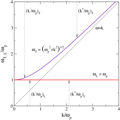
Figure 2: The leading order transverse and longitudinal photon dispersion relations $\omega_{T}$ and $\omega_{L}$ used in the numerical evaluation of the neutrino emissivities. The momentum cut-offs $(k^{\pm}/\omega_{p})_{T,L}$ depend on the density and temperature of the plasma.

The relations in Eqs. (36) and (37) yield

$$m_{k}^{T} = \omega_{p}\,:\hskip 65.44142pt{\rm Transverse}$$ (38)

$$m_{k}^{L} = \sqrt{\omega_{p}^{2}-{\bf|k|}^{2}}\,:\hskip 28.45274pt{\rm Longitudinal}\,.$$ (39)

For the transverse photon, the momentum cutoffs are given by

$$|{\bf k}|^{\pm} = \biggl{[}\biggl{(}\frac{EA\pm|{\bf\bar{P}}|\sqrt{A^{2}-4M^{2}\omega_{p}^{2}}}{2M^{2}}\biggl{)}^{2}-\omega_{p}^{2}\biggr{]}^{1/2}\,,$$ (40)

where $A=M^{2}+\omega_{p}^{2}-m_{e}^{2}$.

For the longitudinal photon (plasmon), the momentum cutoffs are

$$|{\bf k}|^{\pm} = \biggl{[}(2|{\bf P}|^{2}-2\omega_{p}E+A)\pm\sqrt{(2|{\bf P}|^{2}-2\omega_{p}E+A)^{2}-(4\omega_{p}^{2}E^{2}-4\omega_{p}EA+A^{2})}~{}\biggr{]}^{1/2}\,.$$ (41)

The use of the leading order dispersion relations yields sufficiently accurate results except in regions where the plasma frequency becomes large so that the ${\bf k}$ integration enters the region where there are significant deviations from Eqs. (36) and (38).

The transverse photon mass in Eq. (38) is momentum independent and therefore integration over the photon momentum can be replaced by integration over energy with limits provided by Eq. (28). We have verified that the two approaches yield the same result for this case. However, the longitudinal mass in Eq. (39) is momentum dependent and integrating over momentum is a better choice with the limits obtained iteratively from Eq. (29).

The momentum cut-offs $(k^{\pm}/\omega_{p})_{T,L}$ are shown schematically in Fig. 2. Depending on the density and temperature of the plasma, the photo-neutrino rate and emissivity receive significant contributions from space-like momenta (i.e., $|{\bf k}|\geq\omega_{p}$) in the longitudinal case. (In the nondegenerate regime, the time-like component is sub-dominant by more than two orders of magnitude.) This is in contrast to the decay of the longitudinal plasmon, $\gamma^{*}\rightarrow\nu+\bar{\nu}$, which is kinematically forbidden in space-like regions (i.e., $|{\bf k}|\leq\omega_{p}$).

II.4 Notes For Numerical Integration

For performing numerical integration, it is convenient to recast the integrals in Eq. (33) into dimensionless forms by the variable transformations

$$E_{q}=E_{\nu}^{c}\,\,x_{1},\,\,\quad\,\,E_{q^{\prime}}=E_{\nu}^{c}\,\,{x_{2}},\,\,\qquad\,\,\theta_{qq\prime} = \pi\,\,{x_{3}}\,,$$

$$E_{p^{\prime}}=E^{l}_{p^{\prime}}+(E^{h}_{p^{\prime}}-E^{l}_{p^{\prime}})\,\,{x_{4}},\,\,\quad\,\,{\bf|k|}={\bf|k|}^{-}+({\bf|k|}^{+}-{\bf|k|}^{-})\,\,{x_{7}}\,,$$

$$\phi_{e}=2\pi\,\,{x_{5}},\,\,\quad\,\,\theta_{e}=\pi\,\,{x_{6}},\,\,\quad\,\,\phi_{k}=2\pi\,\,{x_{8}}$$ (42)

which results in

$$Q = \frac{(\pi{E_{\nu}^{c}})^{4}}{(2\pi)^{8}}\int_{0}^{1}x_{1}\,dx_{1}\,\,\int_{0}^{1}x_{2}\,dx_{2}\,\,\int_{0}^{1}\sin\,\theta_{qq\prime}\,dx_{3}\,\,\int_{0}^{1}{\bf|p|}^{\prime}\,(E^{h}_{p^{\prime}}-E^{l}_{p^{\prime}})\,\,dx_{4}\int_{0}^{1}\sin\,\theta_{e}\,dx_{6}\,\,$$ (43)

$$\times\int_{0}^{1}\,dx_{5}\,\,[1-F_{e}(E_{p^{\prime})}]\,\,(E_{q}+E_{q^{\prime}})\,\,I(p^{\prime},q,q^{\prime})$$

$$I(p^{\prime},q,q^{\prime}) = \frac{1}{8\pi}\int_{0}^{1}\frac{{\bf|k|}}{\omega}\,\,({\bf|k|}^{+}-{\bf|k|}^{-})\,\,{dx_{7}}\,\,\int_{0}^{1}dx_{8}\,\,F_{\gamma}(\omega)\,\,F_{e}(E_{p})\,\frac{1}{{\bf|P|}}\,\,\sum_{s,\epsilon}|\mathcal{M}^{T\,(L)}|^{2}\,.$$ (44)

The 8-dimensional integral above is readily integrated by Monte Carlo methods. Although importance sampling reduces the variance of the final result, a flat sampling with suitable cut-offs of troublesome integrands yields equally good results. Such cut-offs can be easily identified through physical reasoning.

In the case of degenerate electrons, the distribution function $F_{e}(E_{p},T)$ and the Pauli blocking factor $1-F_{e}(E_{p^{\prime}},T)$ ensure that the relevant integrand peaks when the value of the electron energy is close to the chemical potential $\mu_{e}$. In other words, electrons primarily play the role of a spectator in this process, originating chiefly from the vicinity of the Fermi surface and reabsorbed into nearby available states. In the partially degenerate and nondegenerate cases, the width of the integrand is governed by the temperature $T$. We employ a flat sampling around the electron chemical potential $\mu_{e}$ and the width is taken to be $\simeq 10T$, which gives the range of energy integration for the outgoing electron to be $E_{p^{\prime}}^{\pm}=\mu_{e}\pm 10T$. Note, however, that $m_{e}$ is the natural lower limit for the electron’s energy, and should be employed when necessary.

For neutrinos, the natural upper cutoff is given by the energy that is available in the medium, which in turn is given by the temperature. We can also expect that energy will be simply transformed from the photon to the two neutrinos, since the electron generally plays the role of a perturbed spectator. The energy released in the form of a $\nu\bar{\nu}$ pair cannot greatly exceed the energy scale dictated by the temperature and setting $E_{\nu}^{c}\simeq(10-15)T$ makes a good choice for the integration cutoff. This can also confirmed by inspecting the integrand $dQ/dE_{\nu}$: the integrand has a maximum around zero and decays roughly by 2 orders of magnitude for $E_{\nu}>10T$.

For certain physical conditions in the plasma, $T\gtrsim m_{e}$, and for densities in the range $10^{10}\mathrel{\raisebox{-2.58334pt}{$\stackrel{{\scriptstyle\textstyle<}}{{\sim}}$}}\rho_{B}Y_{e}/{\rm g~{}cm^{-3}}\mathrel{\raisebox{-2.58334pt}{$\stackrel{{\scriptstyle\textstyle<}}{{\sim}}$}}10^{12}$, numerical problems are encountered in using a Monte Carlo procedure to integrate Eq. (33) (see also BEAUDET1 ; BEAUDET2 ; DICUS1 ; BOND1 ; SCHINDER1 ; ITOH in which such difficulties have been reported). In Appendix B, we discuss the cause and remedy of this longstanding problem.

III RESULTS

Our discussion will be restricted to the case of an equilibrium plasma in which the net negative electric charge of electrons and positrons is cancelled by a uniform positively charged background of protons, alpha particles, and heavier ions. The equation of state and the phase structure of matter, and the abundances of the various constituents including those of dripped neutrons at sub-nuclear densities are determined by the minimization of free energy LS .

We will present our results for the total and differential emissivities as a function of the mass density of protons in the plasma, $\rho_{B}Y_{e}=m_{p}n_{e}$, where $m_{p}$ is the proton mass, $Y_{e}=n_{e}/n_{B}$ is the net electron fraction ($n_{B}$ is the baryon number density) , and $n_{e}$ is net electron number density

$$n_{e}(T,\mu_{e}) = \frac{1}{\pi^{2}}\int_{0}^{\infty}dp\,\,p^{2}\left(F_{e^{-}}-F_{e^{+}}\right)\,,$$ (45)

which is simply the difference between the $e^{-}$ and $e^{+}$ number densities. (The quantity $\rho_{B}Y_{e}$ is the same as $\rho/\mu_{e}$ used in prior works including Ref. BRAATEN1 .) Given $n_{e}$, this expression can be inverted to determine the chemical potential $\mu_{e}$ at a given temperature.

Figure 3: The plasma frequency $\omega_{p}$ (upper panel) and the chemical potential $\mu_{e}$ (lower panel) as functions of density for select temperatures. The vertical dashed lines in panel (a) indicate the densities at which $\omega_{p}=T$. The vertical dotted lines mark the turn-on densities at which the plasma frequency and the neutrino emissivity (Fig. 4) abruptly change their behavior from being independent of density.

In order to gain a qualitative understanding of the basic features of $Q_{T}$ and $Q_{L}$ in terms of the intrinsic properties of the plasma, it is instructive to inspect the behaviors of the chemical potential $\mu_{e}$ and plasma frequency $\omega_{p}$ (this is the characteristic energy scale generated by interactions in the medium) as $T$ and $\rho_{B}Y_{e}$ are varied. Figure 3 shows $\mu_{e}$ (lower panel) obtained by inverting Eq. (45) and $\omega_{p}$ (upper panel) calculated from Eq. (59) of Ref. RIP02 . The results of the total emissivities are readily interpreted on the basis of the trends observed in Fig. 3.

Noteworthy features of the plasma frequency in panel (a) of Fig. 3 are:
(1) $\omega_{p}$ is independent of $\rho_{B}Y_{e}$ till the turn-on density $(\rho_{B}Y_{e})_{\rm to}$ is reached (this is at the root of why $Q_{T}$ and $Q_{L}$ are constant for $\rho_{B}Y_{e}<(\rho_{B}Y_{e})_{\rm to}$), and
(2) $\omega_{p}$ shows a power-law increase for $\rho_{B}Y_{e}>(\rho_{B}Y_{e})_{\rm to}$, the index depending both on the extent to which the plasma is in the non-degenerate, partially degenerate or degenerate regime and on whether electrons are relativistic or nonrelativistic.

The bold and light portions of the various curves in panel (b) of Fig. 3 mark the regions of densities for which $\mu_{e}\geq T$ and $\mu_{e}\leq T)$, respectively. Inasmuch as $\mu_{e}\simeq T$ indicates partial degeneracy of the plasma, the bold and light portions refer to the degenerate and non-degenerate conditions, respectively. For reference, the electron mass, which when compared with $\mu_{e}$ or $T$ determines the degree of relativity, is marked by the horizontal dotted line in this figure. The vertical dotted lines show the respective locations of the turn-on densities.

The results of Monte Carlo integrations of the transverse and longitudinal total emissivities in Eq. (43) are shown as a function of baryon density in Fig. 4 for select temperatures. While the emissivities increase rapidly with temperature, their behavior with density is more intricate. At a fixed temperature, the important characteristics to note are:
(1) Both $Q_{T}$ and $Q_{L}$ are independent of the density $\rho_{B}Y_{e}$ until a turn-on density $(\rho_{B}Y_{e})_{\rm to}$ is reached,
(2) For densities larger than this turn-on density, $Q_{T}$ and $Q_{L}$ rise rapidly until they attain their peak values at a density $(\rho_{B}Y_{e})_{\rm peak}$, and
(3) For $\rho_{B}Y_{e}\gg(\rho_{B}Y_{e})_{\rm peak}$, the fall-off with density is exponential.
A conspicuous feature to note is that with increasing temperature, the emissivities show a kinky behavior as they begin to approach their maximum values.

In Fig. 5, the transverse and longitudinal rates, $\Gamma_{T}$ and $\Gamma_{L}$, are shown as functions of density and temperature. The qualitative features of the rates are similar to those noted above for the emissivities.

The physical origins of the basic trends in the emissivities and rates are identified in the following section.

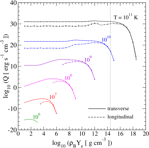
Figure 4: Individual contributions from the transverse and longitudinal channels to the neutrino emissivity as a function of baryon density at the indicated temperatures. The error bars show the variance of the Monte Carlo integration of Eq. (43). For densities in excess of nuclear density shown by the dotted vertical line, neutrino production from strongly interacting particles dominate over QED-plasma processes.

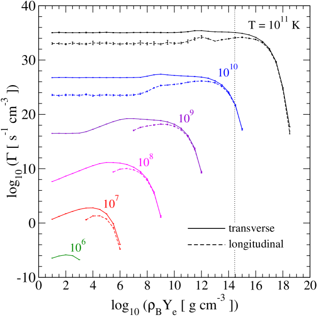
Figure 5: Individual contributions from the transverse and longitudinal channels to the neutrino rates as a function of baryon density at the indicated temperatures. The error bars show the variance of the Monte Carlo integration. For densities in excess of nuclear density shown by the dotted vertical line, neutrino production from strongly interacting particles dominate over QED-plasma processes.

III.1 Analytical Analysis of the Qualitative Behaviours

In order to gain a qualitative, and in many cases quantitative, understanding of the neutrino emissivity as a function of temperature and density, it is useful to identify the dominant physical scales in the photoproduction of neutrino pairs under limiting situations. This can be achieved in the cases of (1) a degenerate plasma, which occurs for all temperatures at sufficiently high densities, and (2) a nondegenerate relativistic plasma in which the density is low, but the temperature is high. Finally, we turn to uncover the origin of the kinks that are conspicuous at high temperatures, but become less prominent at low temperatures.

Since our goal here is to provide order of magnitude estimates to better understand the exact numerical results of the preceding section, we will simplify considerably the integrand in Eq. (33) by
(1) estimating the dominant scales of energies and momenta of the incoming and outgoing particles, and
(2) extensively use physically motivated approximations.
These steps are helpful in taming the formidable 8-dimensional integral in Eq. (33) which cannot be otherwise computed analytically. In the discussion that follows, we will focus on the dominant transverse channel; the analysis for the longitudinal channel can be carried along similar lines.

III.1.1 The Degenerate Case

For all temperatures at sufficiently high net electron densities $n_{e}$, the inequalities

$$\mu_{e}\gg T, \mu_{e}\gg m_{e},\;$$

$$\omega_{P}\gg T, \omega_{P}\gg m_{e}$$ (46)

are satisfied. Thus, the electron chemical potential $\mu_{e}\simeq{(3\pi^{2}n_{e})}^{1/3}$ and the photon effective mass $\omega_{p}\simeq\sqrt{4\alpha/3\pi}\mu_{e}\simeq\mu_{e}/18$ (e.g. see Refs. RIP02 ; BRAATEN1 ) are the dominant energy scales in the problem. Since $T\ll\mu_{e}$, the Pauli-blocking of outgoing electrons ensures that the participating electrons lie close to the Fermi surface. In other words, electrons are elastically scattered, exchanging only the $3$-momentum with the photon and the outgoing neutrinos. Under such circumstances, we can expect the electron energies to be

$$E_{p}\simeq E_{p^{\prime}}\simeq{\bf|p|}\simeq{\bf|p^{\prime}|}\simeq\mu_{e}$$ (47)

for both the incoming and outgoing electrons. This in turn implies that the photon transfers its entire energy to the $\nu{\bar{\nu}}$ pair. The photon energy and momentum are

$$\omega\simeq\omega_{p}\simeq E_{q}+E_{q^{\prime}}\qquad{\rm and}\qquad{\bf|k|}\simeq T\,.$$ (48)

The characteristic components of the outgoing neutrino 4-momentum then become $E_{q}\simeq{\bf|q|}\simeq\omega_{p}/2$. These estimates for the relevant energies and momenta allow us to make an estimate of the squared matrix element. The generic form of the squared matrix element can be written as

$$\sum_{s,\epsilon}{|{\mathcal{M}}^{T}|}^{2} \sim 256\pi\alpha G_{F}^{2}(C_{V}^{2}+C_{A}^{2})\times\frac{1}{(k^{2}\pm 2p_{i}\cdot k)^{2}}\times\{\rm{a~{}6^{th}~{}order~{}polynomial~{}in~{}4-momenta}\}\,,$$ (49)

where the dominant terms in the polynomial consist of 2 powers of $k$ and one power each of $q$, $q^{\prime}$, $p$, and $p^{\prime}$. The contribution from the term involving $m_{e}^{2}(C_{V}^{2}-C_{A}^{2})$ in the squared matrix element can be dropped, since $m_{e}\ll\mu_{e}$. By using power counting combined with our estimates of the relevant energies and momenta ($q_{i}\simeq\omega_{p}/2$, $p_{i}\simeq\mu_{e}$, and $k\simeq\omega_{p}$), the factor involving the polynomial can be approximated by $\sim\mu_{e}^{2}\omega_{p}^{4}/4$.

The factor

$$\frac{1}{\beta_{2}} = \frac{1}{k^{2}-2p^{\prime}\cdot k}$$ (50)

needs more care, since for some ranges of temperature and density it can develop a resonant behavior (see Appendix B for a detailed analysis of the physical conditions for which this can occur). In the absence of such behavior, its magnitude can be estimated by averaging this factor over the appropriate angular variable. The largest contributions can be determined to be

$$\Big{\langle}\frac{1}{\beta_{1}^{2}}\Big{\rangle} \simeq \Big{\langle}\frac{1}{\beta_{2}^{2}}\Big{\rangle}\simeq\Big{\langle}\frac{1}{\beta_{1}\beta_{2}}\Big{\rangle}\simeq\frac{1}{4\mu_{e}^{2}\omega_{p}^{2}}\,.$$ (51)

Using these estimates, the squared transverse matrix element can be approximated by

$$\sum_{s,\epsilon}{|{\mathcal{M}}^{T}|}^{2} \simeq 16\pi\alpha G_{F}^{2}(C_{V}^{2}+C_{A}^{2})\omega_{p}^{2}\,.$$ (52)

The remaining integrals in Eq. (33) for the total emissivity can be performed along the lines outlined in Sec. II. The transverse emissivity then becomes

$$Q_{T} \simeq \frac{\alpha G_{F}^{2}(C_{V}^{2}+C_{A}^{2})\omega_{p}^{2}}{4(2\pi)^{9}}\int\frac{d^{3}q}{E_{q^{\prime}}}\frac{d^{3}q^{\prime}}{E_{q}}\frac{d^{3}p^{\prime}}{E_{p^{\prime}}}(1-F(E_{p^{\prime}}))\frac{1}{|{\bf P}|}\int_{(E-|{\bf P}|)/2}^{(E+|{\bf P}|)/2}dE_{p}\;F(E_{p})\;F_{\gamma}(E_{q}+E_{q^{\prime}})\;(E_{q}+E_{q^{\prime}})\,.$$ (53)

Since we expect that the most beneficial case for the emissivity is when $E_{p}\simeq E_{p^{\prime}}\simeq\mu_{e}$, we can set $F(E_{p})\rightarrow F(E_{p^{\prime}})$. The $dE_{p}$ integration simply yields the range of $E_{p}$ around $\mu_{e}$ for which the integrand is significant; i.e., $\int dE_{p}\simeq T$. The factor $1/|{\bf P}|=1/|{\bf p}+{\bf k}|$ can be approximated by $1/\mu_{e}$, since $|{\bf p}|\simeq\mu_{e}\gg|{\bf k}|$. The $dE_{p^{\prime}}$ integrand is sharply peaked around $E_{p^{\prime}}=\mu_{e}$, so we can set $E_{p^{\prime}}=\mu_{e}$ everywhere except in the distribution functions, whence the $dE_{p^{\prime}}$ integration becomes straightforward. After introducing new variables $x\equiv E_{q}/T$ and $y\equiv E_{q^{\prime}}/T$, and the constant $a\equiv\omega_{p}/T$, Eq. (53) becomes

$$Q_{T} \simeq \frac{2\alpha G_{F}^{2}(C_{V}^{2}+C_{A}^{2})\omega_{p}^{2}T^{7}}{(2\pi)^{6}}\iint_{0}^{\infty}dxdy\,xy(x+y)\,e^{-(x+y)}\,\theta(x+y-a)\,,$$ (54)

where the factor $\theta(x+y-a)$ arises from the condition $E_{q}+E_{q^{\prime}}=\omega\geq\omega_{p}$. The integral above can be expressed as

$$I(a) = \iint_{0}^{\infty}dxdy\,xy(x+y)\,e^{-(x+y)}\,\theta(x+y-a)=\frac{2}{3}\,\Gamma(5,a)\,,$$ (55)

where $\Gamma(5,a)$ is the incomplete gamma function:

$$\Gamma(n,a)=\int_{a}^{\infty}dx\,x^{n-1}\,e^{-x}={(a)}^{n-1}\,e^{-a}\,\sum_{k=0}^{n-1}{\frac{{(a)}^{-k}(n-1)!}{(n-k-1)!}}\,.$$ (56)

The rightmost expression above is an asymptotic expansion. Since in this limit $a=\omega_{p}/T\gg 1$, we can keep only the leading order term in the asymptotic expansion to obtain

$$Q_{T} \simeq \frac{4}{3}\,\frac{\alpha G_{F}^{2}(C_{V}^{2}+C_{A}^{2})}{(2\pi)^{6}}\,\,{\omega_{p}}^{6}\,T^{3}\,e^{-\omega_{p}/T}\,.$$ (57)

Although the emissivity from this expression agrees very well with our numerical results at high densities, it should be emphasized that its utility lies in predicting qualitative trends, since the exact numerical prefactor depends strongly on the approximations employed. However, the $Q_{T}\sim{\omega_{p}}^{6}\,T^{3}\,e^{-\omega_{p}/T}$ dependence can be employed to predict quantitatively the density at which the emissivity reaches its maximum value. From Eq. (57), we obtain

$$(\rho_{B}Y_{e})_{max}\simeq 9.213\times 10^{12}\,{\Big{(}\frac{T}{{\rm MeV}}\Big{)}}^{3}\,\textrm{g cm}^{-3}\,.$$ (58)

At high temperatures ($T\gtrsim 10^{9}$ K) the emissivity has another, slightly higher maximum in the intermediate region where ($\mu_{e}>T>\omega_{p}$). This can significantly broaden the peak and mask the degenerate maximum. However, we can easily recognize the position of the peak corresponding to Eq. (58) by noting that a peak occurs just before the exponential decrease. These positions are accurately predicted by Eq. (58) with inputs for $\omega_{p}$ and $\mu_{e}$ from Fig. 3. At lower temperatures, or in the longitudinal case in the entire temperature range, this intermediate maximum is absent and we can clearly confirm the behaviour predicted by Eq. (57).

Employing the same physical reasoning and analytical approximations that were used in estimating the total transverse emissivity, the total transverse rate turns out to be

$$\Gamma_{T} \simeq \frac{4}{3}\,\frac{\alpha G_{F}^{2}(C_{V}^{2}+C_{A}^{2})}{(2\pi)^{6}}\,\omega_{p}^{2}\,T^{6}\>\Gamma(4,\omega_{p}/T)$$ (59)

$$\approx \frac{4}{3}\,\frac{\alpha G_{F}^{2}(C_{V}^{2}+C_{A}^{2})}{(2\pi)^{6}}\,\omega_{p}^{5}\,T^{3}\>e^{-\omega_{p}/T}\,.$$

III.1.2 The Nondegenerate Case

The nondegenerate situation occurs at sufficiently low densities for which $\mu_{e}-m_{e}\ll T$. In this case, both $Q_{T}$ and $Q_{L}$ exhibit a plateau for temperatures $T\geq 10^{9}$ K. This behavior of the emissivities is intimately connected with a similar behavior of the plasma frequency $\omega_{p}$ for the corresponding temperatures (see Fig. 3). In this case, we can expect that a significant fraction of the electrons participate in energy exchange.

For $T\gtrsim 10^{10}$ K, we can neglect the electron mass ($m_{e}=5.93\times 10^{9}$ K) in comparison to $\mu_{e}$. In the relativistic regime, net electron density and the plasma frequency are given by RIP02 ; BRAATEN1

$$n_{e} = \frac{\mu_{e}}{3\pi^{2}}\biggl{(}\mu_{e}^{2}+T^{2}\pi^{2}\biggr{)}\simeq\frac{\mu_{e}T^{2}}{3}$$

$$\omega_{p}^{2} = \frac{4\alpha}{3\pi}\biggl{(}\mu_{e}^{2}+\frac{\pi^{2}T^{2}}{3}\biggr{)}\simeq\frac{4\pi\alpha T^{2}}{9}\,,$$ (60)

where the rightmost expressions are valid for $T\gg\mu_{e}$. In this case, the characteristic electron energy and momentum are of order $E_{p}\simeq{\bf|p|}\simeq T$, and the photon energy and momentum are $\omega\simeq{\bf|k|}\simeq T$.

Since the temperature becomes the dominant energy scale governing the neutrino-pair emission process, we can use dimensional analysis to establish that the neutrino emissivity and rate will scale with temperature as $T^{9}$ and $T^{8}$, respectively. An analytical estimation of the numerical prefactors, however, needs some work. In this case, we have identified the leading term in the squared transverse matrix element to be

$$\sum_{s,\epsilon}{|{\mathcal{M}}^{T}|}^{2} \simeq 256\,\pi\,\alpha\,G_{F}^{2}\,(C_{V}^{2}+C_{A}^{2})\,\frac{2(p^{\prime}\cdot k)\big{(}(p\cdot q)(k\cdot q^{\prime})+(p\cdot q^{\prime})(k\cdot q)\big{)}}{{(2p^{\prime}\cdot k-k^{2})}^{2}}\,.$$ (61)

The predominance of this term over all other terms is chiefly due to the resonant nature of the denominator. The angular dependences involving the outgoing neutrinos do not have a large effect, whence, to very good approximation we can write

$$\sum_{s,\epsilon}{|{\mathcal{M}}^{T}|}^{2} \simeq 256\,\pi\,\alpha\,G_{F}^{2}\,(C_{V}^{2}+C_{A}^{2})\,\omega E_{p}E_{q}E_{q^{\prime}}\frac{(p^{\prime}\cdot k)}{{(2p^{\prime}\cdot k-k^{2})}^{2}}\,.$$ (62)

We can further use the average value of

$$\frac{(p^{\prime}\cdot k)}{{(2p^{\prime}\cdot k-k^{2})}^{2}} \simeq \frac{1}{2}\int_{-1}^{1}\frac{E_{p^{\prime}}\omega-|{\bf{p^{\prime}}}||{\bf k}|x}{{(2E_{p^{\prime}}\omega-2|{\bf p^{\prime}}||{\bf k}|x-\omega_{p}^{2})}^{2}}\,dx\,,$$ (63)

where $x$ denotes the cosine of the angle between ${\bf p^{\prime}}$ and ${\bf k}$. The value of this integral does not depend sensitively on $\omega_{p}^{2}$, since it is negligibly small compared to the other terms in the denominator. We can therefore set it to zero without significantly changing the final result. In the relativistic regime, we can also ignore the electron mass compared to its typical momentum. We then find

$$\frac{(p^{\prime}\cdot k)}{{(2p^{\prime}\cdot k-k^{2})}^{2}} \simeq \frac{1}{2}\frac{1}{4E_{p^{\prime}}\omega}\ln\left(\frac{4\omega^{2}}{\omega_{p}^{2}}\right)\simeq\frac{1}{E_{p^{\prime}}\omega}\,,$$ (64)

where in obtaining the rightmost result, we have utilized the average energy of an equilibrated nearly massless photon $\langle\omega\rangle=2.7T$ and $\omega_{p}\simeq T/10$ as appropriate for this regime. The working expression for the squared matrix element then becomes

$$\sum_{s,\epsilon}{|{\mathcal{M}}^{T}|}^{2} \simeq 256\,\pi\,\alpha\,G_{F}^{2}\,(C_{V}^{2}+C_{A}^{2})\,\frac{E_{p}E_{q}E_{q^{\prime}}}{E_{p^{\prime}}}\,.$$ (65)

The identity

$$\int\frac{d^{3}q}{2E_{q}}\,\frac{d^{3}q^{\prime}}{2E_{q^{\prime}}}\,\delta^{4}(q+q^{\prime}-q_{t})\,{E_{q}\,E_{q^{\prime}}} = \frac{\pi}{24}\,\Theta(q_{t}^{2})\,(3{q_{t}^{0}}^{2}-|{\bf q_{t}}|^{2})\,,$$ (66)

where the four-vector $q_{t}=(q_{t}^{0},{\bf q_{t}})\equiv q+q^{\prime}=p+k-p^{\prime}$, helps us to write the emissivity and the rate as

$$\genfrac{(}{)}{0.0pt}{}{Q_{T}}{\Gamma_{T}} = \frac{32\pi^{2}\alpha G_{F}^{2}(C_{V}^{2}+C_{A}^{2})}{3(2\pi)^{11}}\int\frac{d^{3}p}{2E_{p}}\,n_{F}(E_{p})\,\frac{d^{3}p^{\prime}}{2E_{p^{\prime}}}\,\left(1-n_{F}(E_{p^{\prime}})\right)\,\frac{d^{3}k}{2\omega}\,n_{B}(\omega)\,$$ (67)

$$\times\,\Theta(q_{t}^{2})\,(3{q_{t}^{0}}^{2}-|{\bf q_{t}}|^{2})\,\frac{E_{p}E_{q}E_{q^{\prime}}}{E_{p^{\prime}}}\,\genfrac{(}{)}{0.0pt}{}{E_{p}+\omega-E_{p^{\prime}}}{1}\,.$$

The remaining integrations are, however, complicated because of the complex integration boundaries arising from the $\Theta(q_{t}^{2})$ factor. In order to simplify this restriction and the integration over the $(3{q_{t}^{0}}^{2}-|{\bf q_{t}}|^{2})$ factor, we use $\Theta(q_{t}^{2})=\Theta(q_{t}^{0}-|{\bf q_{t}}|)$, and replace $|{\bf q_{t}}|$ and $|{\bf q_{t}}|^{2}$ by their average values:

$$\langle|{\bf q_{t}}|\rangle = \frac{1}{2}\int_{-1}^{1}dy\,\sqrt{(E_{q}^{2}+E_{q^{\prime}}^{2}+2E_{q}E_{q^{\prime}}y)}=E_{>}+\frac{1}{3}\frac{E_{<}^{2}}{E_{>}}\simeq q_{t}^{0}/2$$ (68)

$$\langle|{\bf q_{t}}|^{2}\rangle = \frac{1}{2}\int_{-1}^{1}dy\,(E_{q}^{2}+E_{q^{\prime}}^{2}+2E_{q}E_{q^{\prime}}y)={q_{t}^{0}}^{2}-2E_{q}E_{q^{\prime}}\simeq{q_{t}^{0}}^{2}/2\,,$$ (69)

where $y$ denotes the cosine of the angle between the two outgoing neutrinos. In Eq. (68), $E_{>}$ and $E_{<}$ are the larger and smaller of the two energies $E_{q}$ and $E_{q^{\prime}}$, respectively. In the last steps of Eqs. (68) and (69), we have replaced the neutrino energies with their average value $q_{t}^{0}/2$. As a result, the following simplifications can be made:

$$\Theta(q_{t}^{2}) \rightarrow \Theta(q_{t}^{0})$$

$$3{q_{t}^{0}}^{2}-|{\bf q_{t}}|^{2} \rightarrow \langle 3{q_{t}^{0}}^{2}-|{\bf q_{t}}|^{2}\rangle=5{q_{t}^{0}}^{2}/2\,.$$ (70)

We note that the condition $\Theta(q_{t}^{0})=\Theta(E_{p}+w-E_{p^{\prime}})$ has the physical interpretation that the outgoing electron energy cannot exceed the total incoming energy.

The emissivity and rate can now be expressed in terms of the simple expressions

$$\genfrac{(}{)}{0.0pt}{}{Q_{T}}{\Gamma_{T}} = \frac{20\alpha G_{F}^{2}(C_{V}^{2}+C_{A}^{2})}{3(2\pi)^{6}}\,\genfrac{(}{)}{0.0pt}{}{T^{9}{\mathcal{I}}_{Q}}{T^{8}{\mathcal{I}}_{\Gamma}}\,,$$ (71)

where the dimensionless constants are

$$\genfrac{(}{)}{0.0pt}{}{{\mathcal{I}}_{Q}}{{\mathcal{I}}_{\Gamma}} = \int_{0}^{\infty}\frac{dx\,x^{2}}{e^{x}+1}\int_{0}^{\infty}\frac{dy\,y}{e^{y}-1}\int_{0}^{x+y}\frac{dz}{e^{-z}+1}\genfrac{(}{)}{0.0pt}{}{(x+y-z)^{3}}{(x+y-z)^{2}}\,,$$ (72)

and the integration variables are $x\equiv E_{p}/T$, $y\equiv w/T$, and $z\equiv E_{p^{\prime}}/T$. A numerical evaluation of these integrals yields

$$\genfrac{(}{)}{0.0pt}{}{{\mathcal{I}}_{Q}}{{\mathcal{I}}_{\Gamma}} = \genfrac{(}{)}{0.0pt}{}{775.54}{136.50}$$ (73)

and the ratio ${\mathcal{I}}_{Q}/{\mathcal{I}}_{T}=5.68$. Analytical approximations to these integrals can be obtained by the replacement

$$\frac{1}{e^{-z}+1} \rightarrow 1$$ (74)

with the result

$${{\mathcal{I}}_{Q}} = \frac{63}{256}\Gamma(7)\zeta(7)\Gamma(2)\zeta(2)+\frac{37}{32}\Gamma(6)\zeta(6)\Gamma(3)\zeta(3)+\frac{73}{32}\Gamma(5)\zeta(5)\Gamma(4)\zeta(4)=1002.1$$ (75)

$${{\mathcal{I}}_{\Gamma}} = \frac{31}{96}\Gamma(6)\zeta(6)\Gamma(2)\zeta(2)+\frac{19}{16}\Gamma(5)\zeta(5)\Gamma(3)\zeta(3)+\frac{7}{8}\Gamma^{2}(4)\zeta^{2}(4)=172.74$$ (76)

($\Gamma(n)$ and $\zeta(n)$ are the Gamma and Riemann’s zeta functions, respectively) and the ratio ${\mathcal{I}}_{Q}/{\mathcal{I}}_{T}=5.8$ which are reasonably close to the exact numerical results. Using the results in Eq. (73), the emissivity and the rate in the nondegenerate case are

$$Q_{T} \simeq 4.35\times 10^{22}{\left(\frac{T}{\rm MeV}\right)}^{9}\,\rm{erg}\,\rm{cm}^{-3}\,\rm{s}^{-1}\,,$$ (77)

$$\Gamma_{T} \simeq 4.78\times 10^{27}{\left(\frac{T}{\rm MeV}\right)}^{8}\,\rm{cm}^{-3}\,\rm{s}^{-1}\,.$$ (78)

The above estimate for the emissivity is in good agreement with the exact numerical results presented in Fig. 4.

As the density increases, the electron chemical potential and the plasma frequency both begin to increase, and become strongly density dependent. As a result, the emissivity also acquires a strong density dependence. We can expect this change of behaviour to occur when the term involving the chemical potential in Eq. (III.1.2) becomes comparable to the term involving $T^{2}$. In this case,

$${\displaystyle(n_{e})_{\rm to}} \simeq {\displaystyle\frac{T^{3}}{2.72}}\quad{\rm or}$$ (79)

$${\displaystyle\left({\rho_{B}}{Y_{e}}\right)_{\rm to}} \simeq {\displaystyle 8\times 10^{7}\left(\frac{T}{{\rm MeV}}\right)^{3}}~{}{\rm g~{}cm^{-3}}$$

$$\Rightarrow\log_{10}({\rho_{B}}{Y_{e}}) = \left\{\begin{array}[]{ll}10.7&\text{at $T=8.6$ MeV ($10^{11}$ K)}\\ 7.7&\text{at $T=0.86$ MeV}\end{array}\right.$$ (82)

which agrees closely with the turn-on densities in Fig. 4.

III.1.3 Intermediate Case

In the case that $\mu_{e}>T>\omega_{p}$, the emissivity $Q_{T}$ acquires a strong density dependence. In addition, a conspicuous maximum occurs prior to entering the strongly degenerate regime. In this density range, the dominant energies are

electrons: $$E_{p}\simeq{\bf|p|}\simeq\mu_{e}$$

photon: $$\omega\simeq{\bf|k|}\simeq T$$

neutrinos: $$E_{q}\simeq{\bf|q|}\simeq T\,.$$ (83)

With these energy scales, the squared matrix element can be estimated to be

$$\sum_{s,\epsilon}{|{\mathcal{M}}^{T}|}^{2} \sim 256\pi\alpha G_{F}^{2}(C_{V}^{2}+C_{A}^{2})\,\frac{1}{4\mu_{e}T\omega_{p}^{2}}\,T^{4}\,\mu_{e}^{2}\,.$$ (84)

The phase space integration can be performed similarly to the degenerate case with the result

$$Q_{T} \simeq \frac{32}{3}\,\frac{\alpha G_{F}^{2}(C_{V}^{2}+C_{A}^{2})}{(2\pi)^{6}}\,\frac{T^{9}\mu_{e}^{2}}{\omega_{p}^{2}}\,\zeta(5)\,\Gamma(5,\omega_{p}/T)\,.$$ (85)

In the region of maximum emissivity, the ratio $\omega_{p}/T\ll 1$ for the two highest temperatures ($10^{10}$ and $10^{11}$ K). This allows us to expand the incomplete gamma function in terms of this small parameter so that

$$Q_{T} \simeq \frac{768}{3}\,\frac{\alpha G_{F}^{2}(C_{V}^{2}+C_{A}^{2})}{(2\pi)^{6}}\,\frac{T^{9}\mu_{e}^{2}}{\omega_{p}^{2}}\,e^{-\omega_{p}/T}.$$ (86)

For $T=8.6$ MeV, the maximum occurs around $\rho_{B}Y_{e}=10^{12}$ g cm^-3, where we have used $\mu_{e}=46.8$ MeV and $\omega_{p}=2.74$ MeV. By combining these values with Eq. (86), the emissivity can be found to be $\log_{10}Q_{T}=32.06$ in very good agreement that in Fig. 4.

For $T=0.86$ MeV, $Q_{T}$ exhibits a maximum around $\rho_{B}Y_{e}=10^{9}$ g cm^-3. In this case, $\mu_{e}=4.71$ MeV and $\omega_{p}=0.274$ MeV. These values yield $\log_{10}Q_{T}=23.0$, which is slightly larger than the exact numerical result.

The origin of the secondary peak lies in the resonant character of the factor

$$\frac{1}{\beta_{2}^{2}}=\frac{1}{(2E_{p}\omega-2{\bf p}\cdot{\bf k}-\omega_{p}^{2})^{2}}$$ (87)

for the case in which the plasma frequency becomes negligible, but $E_{p}\simeq{\bf|p|}$ and $\omega\simeq{\bf|k|}$. Such conditions cannot be satisfied in a strongly degenerate medium in which $\omega\simeq\omega_{p}\gg k\simeq T$ or at low temperatures for which $E_{p}\simeq m_{e}$ and $|{\bf p}|\simeq T\ll m_{e}$. Hence, as the temperature decreases this enhancement becomes reduced and at $T\lesssim 10^{8}$ K it is completely absent.

This resonant structure also gives rise to numerical problems at high temperatures and is further discussed in Appendix B. Unless suitably accounted for, this factor enhances the variance of the Monte Carlo integration by large factors.

III.2 Typical Neutrino Energies

The mean neutrino plus anti-neutrino energy can be characterized by the ratio of the total emissivity to the total rate. In this section, we analyze

$${\langle E_{\nu\bar{\nu}}\rangle}_{T} = \frac{Q_{T}}{\Gamma_{T}}\,$$ (88)

for the transverse case. The analysis for the longitudinal case can be performed in a similar fashion. Utilizing the numerical results from Eq. (43) and its counterpart for the rate, the exact results for $\langle E_{\nu\bar{\nu}}\rangle_{T}$ versus density at various temperatures are shown by the solid lines in Fig. 6. The discussion below is aimed toward a qualitative understanding of the basic trends in this figure in limiting cases.

In the degenerate case, the results in Eqs. (57) and (59) set the average neutrino pair energy to be

$${\langle E_{\nu\bar{\nu}}\rangle}_{T} \simeq \omega_{p}\,$$ (89)

in line with the assumption that $E_{q}+E_{q^{{}^{\prime}}}\simeq\omega_{p}$ used in the approximation procedure. For the two highest temperatures $T/{\rm MeV}=0.86$ and 8.6 shown in Fig. 6, $\langle E_{\nu\bar{\nu}}\rangle=6.8T$ and $7T$, respectively. From the results in Eqs. (77) and (78) in Sec. III.1.2, we obtain

$${\langle E_{\nu\bar{\nu}}\rangle}_{T} \simeq 5.8\,T\,$$ (90)

in the non-degenerate relativistic case, which, considering the approximations made, is a reasonable estimate.

It is instructive to compare the mean neutrino pair energy ${\langle E_{\nu\bar{\nu}}\rangle}_{T}$ with the characteristic energy of the in-medium photons in the plasma. The average photon energy in the plasma is given by

$$\langle\omega_{T}\rangle = \frac{\displaystyle\int_{0}^{\infty}dk~{}k^{2}\omega_{T}\,F_{\gamma}(\omega_{T},T)}{\displaystyle\int_{0}^{\infty}dk\,k^{2}F_{\gamma}(\omega_{T},T)}\simeq\;\frac{\omega_{p}^{2}}{8T}\;\frac{{\displaystyle\sum_{j=1}^{\infty}}{\displaystyle\biggl{[}}K_{4}(jy)-K_{0}(jy){\displaystyle\biggr{]}}}{{\displaystyle\sum_{j=1}^{\infty}}K_{2}(jy)/j}~{}\,,$$ (91)

where the rightmost relation is obtained upon setting $\omega_{T}^{2}-k^{2}\simeq m_{T}^{2}\approx\omega_{p}^{2}$ (see also Ref. RIP02 ). Simpler results ensue for the extreme relativistic and nonrelativistic cases:

$$\langle\omega_{T}\rangle \simeq 2.7~{}T\qquad\quad{\rm for}\quad T\gg\omega_{p}$$ (92)

$$\simeq \omega_{p}+\frac{3}{2}~{}T\quad\,{\rm for}\quad T\ll\omega_{p}\,.$$ (93)

The dashed curves in Fig. 6 show expectations based on Eq. (91).

Comparing the result in Eq. (90) with that in Eq. (89), we confirm that in the degenerate case the process proceeds as the decay of a massive photon into two neutrinos, with electrons and positrons emerging with modified angles in their final states. The numerical results in the figure also support this expectation. Notice, however, that as the density is progressively increased, the average neutrino energy becomes somewhat smaller than the average photon energy. This can be attributed to the fact that some of the available energy is taken by the outgoing electrons.

In the relativistic case, the average neutrino pair energy (Eq. (90)) is significantly enhanced relative to the average photon energy (Eq. (92)). This can be attributed to the different energy weightings of the squared matrix element in $Q_{T}$ and $\Gamma_{T}$ not accounted for in Eq. (91) and to the fact that electrons and positrons impart some of their energy to the neutrino pair.

Figure 6: Average transverse photon and neutrino pair energies as functions of density and temperature.

IV Kernels for Neutrino Transport Calculations

The matrix elements derived in Sec. II enable us to obtain the source and sink terms associated with the photo-neutrino process which are required in neutrino transport calculations. The evolution of the neutrino distribution function $f$, generally described by the Boltzmann transport equation in conjunction with hydrodynamical equations of motion together with baryon and lepton number conservation equations is

$$\frac{\partial f}{\partial t}+v^{i}\frac{\partial f}{\partial x^{i}}+\frac{\partial(fF^{i})}{\partial p^{i}}=B_{EA}(f)+B_{NES}(f)+B_{\nu{\cal N}}(f)+B_{TP}(f)\,.$$ (94)

Here, $F^{i}$ is the force acting on the particle and we have ignored general relativistic effects for simplicity (see, for example, Ref. BRUENN1 for full details). The right hand side of the above equation is the neutrino source term in which, $B_{EA}(f)$ incorporates neutrino emission and absorption processes, $B_{NES}(f)$ accounts for the neutrino-electron scattering process, $B_{\nu{\cal N}}(f)$ includes scattering of neutrinos off nucleons and nuclei, and $B_{TP}(f)$ considers the thermal production and absorption of neutrino-antineutrino pairs.

In this section, we obtain the contribution from the photo-neutrino process to the thermal production term $B_{TP}$. In doing so, we follow closely Ref. RIP02 where kernels for the plasma process and Ref. BRUENN1 in which neutrino pair production from $e^{+}e^{-}$ annihilation were obtained. Suppressing the dependencies on $(r,t)$ for notational simplicity, the source term for the photo-neutrino process can be written as

$$B\big{(}f(\mu_{q},E_{q})\big{)} = \biggl{[}1-f(\mu_{q},E_{q})\biggr{]}\frac{1}{(2\pi)^{3}}\int_{0}^{\infty}E^{2}_{q^{\prime}}\,\,dE_{q^{\prime}}\int_{-1}^{1}d\mu_{q^{\prime}}\int_{0}^{2\pi}d\phi_{q^{\prime}}\,R^{p}\biggl{(}E_{q},E_{q^{\prime}},\cos\,\theta_{qq\prime}\biggr{)}\,\biggl{[}1-\bar{f}(\mu_{q^{\prime}},E_{q^{\prime}})\biggr{]}$$ (95)

$$- f(\mu_{q},E_{q})\frac{1}{(2\pi)^{3}}\int_{0}^{\infty}E^{2}_{q^{\prime}}\,\,dE_{q^{\prime}}\int_{-1}^{1}d\mu_{q^{\prime}}\int_{0}^{2\pi}d\phi_{q^{\prime}}\,R^{a}\biggl{(}E_{q},E_{q^{\prime}},\cos\,\theta_{qq\prime}\biggr{)}\,\bar{f}(\mu_{q^{\prime}},E_{q^{\prime}})\,,$$

where the first and the second terms correspond to the source (neutrino gain) and sink (neutrino loss) terms, respectively. Angular variables $\mu_{q(q^{\prime})}\equiv\cos\theta_{q(q^{\prime})}$ and $\phi_{q(q^{\prime})}$ are defined with respect to the $z$-axis that is locally set parallel to the outgoing radial vector ${\bf r}$. The angle $\theta_{qq\prime}$ between the neutrino and antineutrino pair is related to $\theta_{q}$ and $\theta_{q^{\prime}}$ through

$$\cos\theta_{qq\prime} = \mu_{q}\mu_{q^{\prime}}+\sqrt{(1-\mu_{q}^{2})(1-\mu_{q^{\prime}}^{2})}~{}\cos(\phi_{q}-\phi_{q^{\prime}})\,.$$ (96)

The production kernel is given by

$$R^{p}(E_{q},E_{q^{\prime}},\cos\theta_{qq\prime})=\int\frac{2d^{3}{\bf p}}{(2\pi)^{3}}\frac{F_{e}(E_{p})}{2E_{p}}\int\frac{\xi d^{3}{\bf k}}{(2\pi)^{3}}\frac{F_{\gamma}(\omega)}{2\omega}\int\frac{d^{3}{\bf p^{\prime}}}{(2\pi)^{3}}\frac{[1-F_{e}(E_{p^{\prime}})]}{2E_{p^{\prime}}}\frac{(2\pi)^{4}}{4E_{q}E_{q^{\prime}}}\delta^{4}(p+k-p^{\prime}-q-q^{\prime})\frac{1}{\zeta}\sum_{s,\epsilon}|{\mathcal{M}}|^{2}\,.$$ (97)

The corresponding expression for the absorption kernel $R^{a}(E_{q},E_{q^{\prime}},\cos\theta_{qq\prime})$ can be obtained by the replacements

$$F_{e}(E_{p})\rightarrow 1-F_{e}(E_{p})\,,\qquad F_{\gamma}(\omega)\rightarrow 1+F_{\gamma}(\omega)\,,\qquad{\rm and}\qquad 1-F_{e}(E_{p^{\prime}})\rightarrow F_{e}(E_{p^{\prime}})\,.$$

The angular dependences in the kernels $R^{\genfrac{}{}{0.0pt}{}{p}{a}}(E_{q},E_{q^{\prime}},\cos\theta_{qq\prime})$ are often expressed in terms of Legendre polynomials as

$$R^{\genfrac{}{}{0.0pt}{}{p}{a}}(E_{q},E_{q^{\prime}},\cos\theta_{qq\prime}) = \sum_{l=0}^{\infty}\frac{2l+1}{2}\Phi^{\genfrac{}{}{0.0pt}{}{p}{a}}_{l}(E_{q},E_{q^{\prime}})P_{l}(\cos\theta_{qq\prime})\,,$$ (98)

where the Legendre coefficients $\Phi^{\genfrac{}{}{0.0pt}{}{p}{a}}_{l}(E_{q},E_{q^{\prime}})$ depend exclusively on energies.

From Eq. (97), it is evident that the kernels are related to the neutrino rates and emissivities. We first consider the production kernel $R^{p}(E_{q},E_{q^{\prime}},\cos\theta_{qq\prime})$. The corresponding analysis for the absorption kernel $R^{a}(E_{q},E_{q^{\prime}},\cos\theta_{qq\prime})$ can be made along the same lines. The neutrino production rate is given by

$$\Gamma = \int\frac{2\,d^{3}{\bf p}}{(2\pi)^{3}}\frac{F_{e}(E_{p})}{2E_{p}}\int\frac{\xi\,d^{3}{\bf k}}{(2\pi)^{3}}\frac{F_{\gamma}(\omega)}{2\omega}\int\frac{d^{3}{\bf p^{\prime}}}{(2\pi)^{3}}\frac{[1-F_{e}(E_{p^{\prime}})]}{2E_{p^{\prime}}}\int\frac{d^{3}{\bf q}}{(2\pi)^{3}}\frac{1}{2E_{q}}\int\frac{d^{3}{\bf q^{\prime}}}{(2\pi)^{3}}\frac{1}{2E_{q^{\prime}}}$$ (99)

$$\times\,\,(2\pi)^{4}\delta^{4}(p+k-p^{\prime}-q-q^{\prime})\,\frac{1}{\zeta}\sum_{s,\epsilon}|{\mathcal{M}}|^{2}\,.$$

$$= \int\frac{d^{3}{\bf q}}{(2\pi)^{3}}\frac{d^{3}{\bf q}^{\prime}}{(2\pi)^{3}}R^{p}(E_{q},E_{q^{\prime}},\cos\theta_{qq\prime})\,,$$ (100)

which defines the kernel $R^{p}(E_{q},E_{q^{\prime}},\cos\theta_{qq\prime})$ and is to be identified with that in Eq. (97). The emissivity $Q$ can also be cast in terms of $R^{p}$ using

$$Q=\int\frac{d^{3}{\bf q}}{(2\pi)^{3}}\frac{d^{3}{\bf q}^{\prime}}{(2\pi)^{3}}(E_{q}+E_{q^{\prime}})R^{p}(E_{q},E_{q^{\prime}},\cos\theta_{qq\prime})\,.$$ (101)

Equations (99) and (101) can be inverted to obtain

$$R^{p}(E_{q},E_{q^{\prime}},\cos\theta_{qq\prime}) = \frac{8\pi^{4}}{E_{q}^{2}E_{q^{\prime}}^{2}}~{}\frac{d^{3}\Gamma}{dE_{q}dE_{q^{\prime}}d\cos\theta_{qq\prime}}$$ (102)

$$= \frac{8\pi^{4}}{E_{q}^{2}E_{q^{\prime}}^{2}(E_{q}+E_{q^{\prime}})}~{}\frac{d^{3}Q}{dE_{q}dE_{q^{\prime}}d\cos\theta_{qq\prime}}\,.$$

Combining Eq. (34) with the above equation, the production kernel can be written as

$$R^{p}(E_{q},E_{q^{\prime}},\cos\theta_{qq\prime})=\frac{\pi^{3}}{(2\pi)^{6}E_{q}E_{q^{\prime}}}\int_{0}^{\infty}\frac{{\bf|p^{\prime}|}^{2}}{E_{p^{\prime}}}d{\bf|p|}^{\prime}\int_{-1}^{1}d\cos\,\theta_{e}\int_{0}^{2\pi}d\phi_{e}[1-F_{e}(E_{p^{\prime}})]I(p^{\prime},q,q^{\prime})$$ (103)

where $I(p^{\prime},q,q^{\prime})$ is given by

$$I(p^{\prime},q,q^{\prime})=\frac{1}{4(2\pi)^{2}}\int_{0}^{\infty}\frac{{\bf|k|}}{\omega}d{\bf|k|}\int_{0}^{2\pi}d\phi\,\,F_{\gamma}(\omega)\,\,F_{e}(E_{p})\,\frac{1}{{\bf|P|}}\,\,\sum_{s,\epsilon}|{\mathcal{M}}|^{2}\,.$$ (104)

The Legendre coefficients $\Phi^{\genfrac{}{}{0.0pt}{}{p}{a}}_{l}(E_{q},E_{q^{\prime}})$ are determined from

$$\Phi^{\genfrac{}{}{0.0pt}{}{p}{a}}_{l}(E_{q},E_{q^{\prime}}) = \int_{-1}^{1}d(\cos\theta_{qq\prime})P_{l}(\cos\theta_{qq\prime})R^{\genfrac{}{}{0.0pt}{}{p}{a}}(E_{q},E_{q^{\prime}},\cos\theta_{qq\prime})\,.$$ (105)

Using Eq. (103) in Eq. (105), the Legendre coefficient for the production process can be expressed as

$$\Phi^{p}_{l}(E_{q},E_{q^{\prime}}) = \frac{\pi^{3}}{(2\pi)^{6}E_{q}E_{q^{\prime}}}\int_{-1}^{1}d(\cos\theta_{qq\prime})P_{l}(\cos\theta_{qq\prime})\int_{0}^{\infty}\frac{{\bf|p^{\prime}|}^{2}}{E_{p^{\prime}}}d{\bf|p|}^{\prime}\int_{-1}^{1}d\cos\,\theta_{e}\int_{0}^{2\pi}d\phi_{e}[1-F_{e}(E_{p^{\prime}})]I(p^{\prime},q,q^{\prime})\,,$$

where $I(p^{\prime},q,q^{\prime})$ is given by Eq. (104).

Numerical results

The structure of the squared matrix element allows us to decompose the Legendre coefficients into parts that are symmetric and anti-symmetric in the energies $E_{q}$ and $E_{q}^{\prime}$ of the two outgoing neutrinos. For example,

$$\Phi_{l}^{p}(E_{q},E_{q^{\prime}}) = (C_{V}^{2}+C_{A}^{2})\times\{\textrm{part symmetric in }(E_{q},\,E_{q^{\prime}})\}$$ (107)

$$+(C_{V}^{2}-C_{A}^{2})\times\{\textrm{part symmetric in }(E_{q},\,E_{q^{\prime}})\}$$

$$+C_{V}C_{A}\times\{\textrm{part antisymmetric in }(E_{q},\,E_{q^{\prime}})\}\,,$$

where only the parts symmetric in $E_{q}$ and $E_{q}^{\prime}$ contribute to the total emissivity $Q$ and rate $\Gamma$, since the anti-symmetric part can be eliminated by the use of Lenard’s identity BEAUDET1 ; DICUS1 ; SCHINDER1 . Furthermore, it is clear from Eq. (98) that only $\Phi^{p}_{0}(E_{q},E_{q^{\prime}})$ contributes to the total emissivity $Q$ and rate $\Gamma$; terms with $l\geq 1$ contribute only to the angular distribution.

Figure 7: Symmetric and anti-symmetric parts of the Legendre coefficients $\Phi_{l}^{p\,({\rm sym})}$ and $\Phi_{l}^{p\,({\rm asym})}$ in the production kernels for the transverse case. The neutrino energies $E_{q}$ and $E_{q^{\prime}}$ are in MeV and the Legendre coefficients are in units of $10^{57}$ $\hbar^{6}$ erg^-6 cm³ s^-7.

In order to ascertain the importance of the $l\geq 1$ coefficients relative to the $l=0$ coefficient, numerical integrations of the integrals in Eq. (IV) were performed for various values of $l$ for the transverse case. Convergent numerical results were obtained by using three different methods: (1) a Monte Carlo procedure with uniform sampling using $10^{5}-10^{6}$ points, (2) the VEGAS Monte Carlo NR procedure that employs stratified importance sampling, and (3) Gauss-Legendre quadrature with 8 and 16 points in each dimension. In regions of density and temperature where the resonant character of the squared matrix element does not become prominent (see Appendix B), the standard Monte Carlo and VEGAS procedures yield similar variances ($\leq 5$%). However, a blind use of the VEGAS routine from standard libraries fails to evaluate the integrals properly in the high $T$ and $\rho_{B}$ regions in which the resonant character of the squared matrix element strikes. As discussed in Appendix B, special care has to be exercised in treating this situation.

Numerical results for the symmetric and anti-symmetric components of $\Phi_{0}^{p}(E_{q},E_{q^{\prime}})$ and $\Phi_{1}^{p}(E_{q},E_{q^{\prime}})$ are shown in Fig. 7 for the case $T=10^{11}$ K$=8.62$ MeV and $\rho_{B}Y_{e}=1$ g cm^-3. The results explicitly show the expected symmetry properties in $E_{q}$ and $E_{q^{\prime}}$. A comparison of the relative magnitudes in these four cases shows that $\Phi_{0}^{p\,({\rm sym})}(E_{q},E_{q^{\prime}})$ is the dominant term. The magnitude of $\Phi_{0}^{p\,({\rm asym})}$ amounts to only 10% of the leading $\Phi_{0}^{p\,({\rm sym})}$ contribution. The contributions of $\Phi_{1}^{p\,({\rm sym})}$ and $\Phi_{1}^{p\,({\rm asym})}$ are 6% and 3%, respectively. In physical terms, this means that neutrino-pair emission from the photo-neutrino process is dominantly isotropic. Therefore, depending on the required accuracy, $\Phi_{0}^{p\,({\rm sym})}$ might be adequate in practical applications. Note also that that the production kernels are negligible for energies $E_{q}$ and $E_{q^{\prime}}$ $\gtrsim 10T$.

V Summary and Relation to Previous Works

In summary, we have calculated the differential rates and emissivities of neutrino pairs from the photo-neutrino process $e^{\pm}+\gamma\rightarrow e^{\pm}+\nu+\bar{\nu}$ in an equilibrium plasma for widely varying baryon densities and temperatures encountered in astrophysical systems. The new analytical expressions for the differential emissivities yield total emissivities that are consistent with those calculated in prior works BEAUDET1 ; BEAUDET2 ; DICUS1 ; BOND1 ; SCHINDER1 ; ITOH . In order to obtain these results, hitherto unavailable squared matrix elements for this process were calculated for the transverse, longitudinal, and mixed components.

We have developed new analytical expressions for the total emissivities in various limiting situations. These results help us to better understand qualitatively, and in many cases quantitatively, the scaling of the results with physical quantities such as the chemical potential and plasma frequency at each temperature and density.

Using our results for the differential rates and emissivities, we have calculated the production and absorption kernels in the source term of the Boltzmann equation employed in exact, albeit numerical, treatments of multienergy neutrino transport. We have also provided the appropriate Legendre coefficients of these kernels in forms suitable for multigroup flux-limited diffusion schemes.

Beginning with the seminal work in Ref. BEAUDET1 , all prior works BEAUDET2 ; DICUS1 ; BOND1 ; SCHINDER1 ; ITOH have concentrated on providing improved total rates and emissivities, but only for the transverse component. Our results for the total emissivity show that the peak values of the longitudinal component are nearly equal to those of the transverse component at all temperatures. (The mixed component vanishes exactly for the total emissivity, but not for the differential emissivity.) Through the years, prior works have persistently reported numerical difficulties in obtaining accurate results at high temperatures and high density. In this work, the cause of these difficulties has been traced to resonant factors that misbehave when Monte Carlo techniques are employed to perform multidimensional integrals. We have overcome these difficulties by utilizing a principal value prescription. The prinicpal new elements of this work are calculations of the full matrix elements, the neutrino differential rates and emissivities, the analytical analysis of the total emissivities in limiting situations, the development of production and absorption kernels in the source term of the Boltzmann equation for neutrino transport, and calculations of the appropriate Legendre coefficients of these kernels in forms suitable for multigroup flux-limited diffusion schemes.

Appendix A Squared Matrix Elements

The squared matrix element in Eq. (12) contains the quantities $\mathcal{M_{-}},\,\mathcal{M_{+}}$ and $\mathcal{M_{\times}}$ which depend on the scalar products of the various four momenta and the polarization of the photon. The fruits of our toil are summarized by the following explicit expressions for these quantities.

$$\mathcal{M_{-}} = -q\cdot q^{\prime}\biggl{[}k^{2}\epsilon\cdot\epsilon\,\,\mathcal{B_{-}}^{2}+4\biggl{(}\frac{\epsilon\cdot p^{2}}{\beta_{1}^{2}}\,\,+\,\,\frac{\epsilon\cdot p{{}^{\prime 2}}}{\beta_{2}^{2}}+\frac{2\epsilon\cdot p\epsilon\cdot p^{\prime}}{\beta_{1}\beta_{2}}\biggr{)}\biggr{]}-4\biggl{[}\frac{k\cdot qk\cdot q^{\prime}\epsilon\cdot\epsilon+k^{2}\epsilon\cdot q\epsilon\cdot q^{\prime}}{\beta_{1}\beta_{2}}\biggr{]}$$ (108)

$$\mathcal{M_{+}} = S(p,p^{\prime},q,q^{\prime})\biggl{[}k^{2}\epsilon\cdot\epsilon\,\,\mathcal{B_{+}}^{2}+4\biggl{(}\frac{\epsilon\cdot p^{2}}{\beta_{1}^{2}}+\frac{\epsilon\cdot p{{}^{\prime 2}}}{\beta_{2}^{2}}+\frac{2\epsilon\cdot p\epsilon\cdot p^{\prime}}{\beta_{1}\beta_{2}}\biggr{)}\biggl{]}$$

$$+2S(k,p^{\prime},q,q^{\prime})\biggl{[}\frac{2\epsilon\cdot p}{\beta_{1}}\biggl{(}\frac{\epsilon\cdot p}{\beta_{1}}+\frac{\epsilon\cdot p^{\prime}}{\beta_{2}}\biggl{)}-\frac{k\cdot p\epsilon\cdot\epsilon}{\beta_{1}}\,\,\mathcal{B_{+}}\biggr{]}-2S(k,p,q,q^{\prime})\biggl{[}\frac{2\epsilon\cdot p^{\prime}}{\beta_{2}}\biggl{(}\frac{\epsilon\cdot p}{\beta_{1}}+\frac{\epsilon\cdot p^{\prime}}{\beta_{2}}\biggl{)}+\frac{k\cdot p^{\prime}\epsilon\cdot\epsilon}{\beta_{2}}\,\,\mathcal{B_{+}}\biggr{]}$$

$$+\frac{4}{\beta_{1}\beta_{2}}\biggl{[}\epsilon\cdot p^{\prime}\epsilon\cdot q^{\prime}\,\,W(p,q,P_{t})+\epsilon\cdot p^{\prime}\epsilon\cdot q\,\,W(p,q^{\prime},P_{t})+\epsilon\cdot p\epsilon\cdot q^{\prime}\,\,W(p^{\prime},q,-P_{t})+\epsilon\cdot p\epsilon\cdot q\,\,W(p^{\prime},q^{\prime},-P_{t})$$

$$-\epsilon\cdot p^{\prime}\epsilon\cdot p(2k\cdot qk\cdot q^{\prime}-k^{2}q\cdot q^{\prime})+\epsilon\cdot q^{\prime}\epsilon\cdot q(k^{2}p\cdot p^{\prime}-2p\cdot kp^{\prime}\cdot k)-\epsilon\cdot\epsilon\biggl{(}q\cdot q^{\prime}(k^{2}p\cdot p^{\prime}-p\cdot kp^{\prime}\cdot k)-p\cdot p^{\prime}k\cdot qk\cdot q^{\prime}\biggr{)}\biggr{]}$$

$${\mathcal{M_{\times}}} = \frac{2}{\beta_{1}^{2}}\biggl{[}(k^{2}\epsilon\cdot\epsilon+4\epsilon\cdot p^{2})\,R(p^{\prime},p,q,q^{\prime})+2\epsilon\cdot p\,\beta_{1}\,(p^{\prime}\cdot q^{\prime}\epsilon\cdot q-p^{\prime}\cdot q\epsilon\cdot q^{\prime})+(-2p\cdot k\epsilon\cdot\epsilon+4\epsilon\cdot p^{2})R(p^{\prime},k,q,q^{\prime})\biggr{]}$$ (110)

$$+\frac{2}{\beta_{2}^{2}}\biggl{[}(k^{2}\epsilon\cdot\epsilon+4\epsilon\cdot p^{\prime 2})R(p^{\prime},p,q,q^{\prime})-2\epsilon\cdot p^{\prime}\,\beta_{2}\,(p\cdot q^{\prime}\epsilon\cdot q-p\cdot q\epsilon\cdot q^{\prime})-(-2p^{\prime}\cdot k\epsilon\cdot\epsilon-4\epsilon\cdot p^{\prime 2})R(p,k,q,q^{\prime})\biggr{]}$$

$$+\frac{4}{\beta_{1}\beta_{2}}Tr\biggl{[}2\epsilon\cdot p^{\prime}\epsilon\cdot p\biggl{(}R(p^{\prime},k,q,q^{\prime})+2R(p^{\prime},p,q,q^{\prime})+R(p,k,q,q^{\prime})\biggr{)}$$

$$-\epsilon\cdot\epsilon\biggl{(}k\cdot p^{\prime}R(p,k,q,q^{\prime})+k^{2}R(p^{\prime},p,q,q^{\prime})-p\cdot kR(p^{\prime},k,q,q^{\prime})\biggr{)}$$

$$+\epsilon\cdot p\epsilon\cdot q\biggl{(}2p^{\prime}\cdot kk\cdot q^{\prime}+2k\cdot p^{\prime}p\cdot q^{\prime}-p^{\prime}\cdot q^{\prime}k^{2}\biggr{)}-\epsilon\cdot p\epsilon\cdot q^{\prime}\biggl{(}2p^{\prime}\cdot kk\cdot q+2k\cdot p^{\prime}p\cdot q-p^{\prime}\cdot qk^{2}\biggr{)}$$

$$+\epsilon\cdot p^{\prime}\epsilon\cdot q^{\prime}\biggl{(}2p\cdot k\,k\cdot q-2p^{\prime}\cdot qp\cdot k-p\cdot qk^{2}\biggr{)}-\epsilon\cdot p^{\prime}\epsilon\cdot q\biggl{(}2p\cdot k\,k\cdot q^{\prime}-2p\cdot kp^{\prime}\cdot q^{\prime}-p\cdot q^{\prime}k^{2}\biggr{)}\biggr{]}$$

In writing the above expressions, we have employed the following notations:

$$P_{t}=p+p^{\prime}\,,\qquad{\mathcal{B_{-}}} = \frac{1}{\beta_{1}}-\frac{1}{\beta_{2}}\,,\qquad{\mathcal{B_{+}}}=\frac{1}{\beta_{1}}+\frac{1}{\beta_{2}}\,,$$

$$S(x,y,w,z) = (x\cdot w)\,\,(y\cdot z)+(x\cdot z)\,\,(y\cdot w)\,,$$

$$R(x,y,w,z) = (x\cdot w)\,\,(y\cdot z)-(x\cdot z)\,\,(y\cdot w)\,,\quad{\rm and}$$

$$W(x,y,z) = (x\cdot k)\,\,(y\cdot k)-(x\cdot y)\,\,k^{2}-(x\cdot k)\,\,(z\cdot y)\,.$$ (111)

After summing over the polarization of the photon, the transverse and longitudinal components of the quantities ${\mathcal{M_{-}}}^{T(L)},\,{\mathcal{M_{+}}}^{T(L)}$ and ${\mathcal{M_{\times}}}^{T(L)}$ required in the calculation of the squared matrix elements in Eq. (19) are

$${\mathcal{M_{-}}}^{T} = 2q\cdot q^{\prime}\biggl{[}k^{2}\,\,\mathcal{B_{-}}^{2}-2\biggl{(}\frac{P^{T}(p,p)}{\beta_{1}^{2}}\,\,+\,\,\frac{P^{T}(p^{\prime},p^{\prime})}{\beta_{2}^{2}}+\frac{2P^{T}(p,p^{\prime})}{\beta_{1}\beta_{2}}\biggr{)}\biggr{]}+4\biggl{[}\frac{2k\cdot qk\cdot q^{\prime}-k^{2}P^{T}(q,q^{\prime})}{\beta_{1}\beta_{2}}\biggr{]}$$ (112)

$${\mathcal{M_{+}}}^{T} = 2S(p,p^{\prime},q,q^{\prime})\biggl{[}-k^{2}\,\,\mathcal{B_{+}}^{2}+2\biggl{(}\frac{P^{T}(p,p)}{\beta_{1}^{2}}\,\,+\,\,\frac{P^{T}(p^{\prime},p^{\prime})}{\beta_{2}^{2}}+\frac{2P^{T}(p,p^{\prime})}{\beta_{1}\beta_{2}}\biggr{)}\biggl{]}$$

$$+4S(k,p^{\prime},q,q^{\prime})\biggl{[}\frac{k\cdot p}{\beta_{1}}\,\,\mathcal{B_{+}}+\frac{1}{\beta_{1}}\biggl{(}\frac{P^{T}(p,p)}{\beta_{1}}+\frac{P^{T}(p,p^{\prime})}{\beta_{2}}\biggl{)}\biggr{]}$$

$$+4S(k,p,q,q^{\prime})\biggl{[}\frac{k\cdot p^{\prime}}{\beta_{2}}\,\,\mathcal{B_{+}}-\frac{1}{\beta_{2}}\biggl{(}\frac{P^{T}(p,p^{\prime})}{\beta_{1}}+\frac{P^{T}(p^{\prime},p^{\prime})}{\beta_{2}}\biggl{)}\biggr{]}$$

$$+\frac{4}{\beta_{1}\beta_{2}}\biggl{[}P^{T}(p^{\prime},q^{\prime})\,W(p,q,P_{t})+P^{T}(p^{\prime},q)\,W(p,q^{\prime},P_{t})+P^{T}(p,q^{\prime})\,W(p^{\prime},q,-P_{t})+P^{T}(p,q)\,W(p^{\prime},q^{\prime},-P_{t})$$

$$-P^{T}(p,p^{\prime})(2k\cdot qk\cdot q^{\prime}-k^{2}q\cdot q^{\prime})+P^{T}(q,q^{\prime})(k^{2}p\cdot p^{\prime}-2p\cdot kp^{\prime}\cdot k)+2q\cdot q^{\prime}(k^{2}p\cdot p^{\prime}-p\cdot kp^{\prime}\cdot k)-2p\cdot p^{\prime}k\cdot qk\cdot q^{\prime}\biggr{]}\,.$$

$${\mathcal{M_{\times}}}^{T} = \frac{2}{\beta_{1}^{2}}\biggl{\{}\biggl{(}-2k^{2}+4P_{T}(p,p)\biggr{)}\,R(p^{\prime},p,q,q^{\prime})+2\beta_{1}\biggl{(}p^{\prime}\cdot q^{\prime}P_{T}(p,q)-p^{\prime}\cdot qP_{T}(p,q^{\prime})\biggr{)}$$ (114)

$$+\biggl{(}4p\cdot k+4P_{T}(p,p)\biggr{)}R(p^{\prime},k,q,q^{\prime})\biggr{\}}$$

$$+\frac{2}{\beta_{2}^{2}}\biggl{\{}\biggl{(}-2k^{2}+4P_{T}(p^{\prime},p^{\prime})\biggr{)}R(p^{\prime},p,q,q^{\prime})-2\beta_{2}\biggl{(}p\cdot q^{\prime}P_{T}(p^{\prime},q)-p\cdot qP_{T}(p^{\prime},q^{\prime})\biggr{)}$$

$$-\biggl{(}4p^{\prime}\cdot k-4P_{T}(p^{\prime},p^{\prime})\biggr{)}R(p,k,q,q^{\prime})\biggr{\}}$$

$$+\frac{4}{\beta_{1}\beta_{2}}\biggl{\{}2P_{T}(p,p^{\prime})\biggl{(}R(p^{\prime},k,q,q^{\prime})+2R(p^{\prime},p,q,q^{\prime})+R(p,k,q,q^{\prime})\biggr{)}$$

$$+2\biggl{(}k\cdot p^{\prime}R(p,k,q,q^{\prime})+k^{2}R(p^{\prime},p,q,q^{\prime})-p\cdot kR(p^{\prime},k,q,q^{\prime})\biggr{)}$$

$$+P_{T}(p,q)\biggl{(}2p^{\prime}\cdot kk\cdot q^{\prime}+2k\cdot p^{\prime}p\cdot q^{\prime}-p^{\prime}\cdot q^{\prime}k^{2}\biggr{)}-P_{T}(p,q^{\prime})\biggl{(}2p^{\prime}\cdot kk\cdot q+2k\cdot p^{\prime}p\cdot q-p^{\prime}\cdot qk^{2}\biggr{)}$$

$$+P_{T}(p^{\prime},q^{\prime})\biggl{(}2p\cdot k\,k\cdot q-2p^{\prime}\cdot qp\cdot k-p\cdot qk^{2}\biggr{)}-P_{T}(p^{\prime},q)\biggl{(}2p\cdot k\,k\cdot q^{\prime}-2p\cdot kp^{\prime}\cdot q^{\prime}-p\cdot q^{\prime}k^{2}\biggr{)}\biggr{\}}$$

The corresponding expressions for the longitudinal component are

$${\mathcal{M_{-}}}^{L} = q\cdot q^{\prime}\biggl{[}k^{2}\,\,\mathcal{B_{-}}^{2}-4\biggl{(}\frac{P^{L}(p,p)}{\beta_{1}^{2}}\,\,+\,\,\frac{P^{L}(p^{\prime},p^{\prime})}{\beta_{2}^{2}}+\frac{2P^{L}(p,p^{\prime})}{\beta_{1}\beta_{2}}\biggr{)}\biggr{]}+4\biggl{[}\frac{k\cdot qk\cdot q^{\prime}-k^{2}P^{L}(q,q^{\prime})}{\beta_{1}\beta_{2}}\biggr{]}$$ (115)

$${\mathcal{M_{+}}}^{L} = S(p,p^{\prime},q,q^{\prime})\biggl{[}-k^{2}\,\,\mathcal{B_{+}}^{2}+4\biggl{(}\frac{P^{L}(p,p)}{\beta_{1}^{2}}\,\,+\,\,\frac{P^{L}(p^{\prime},p^{\prime})}{\beta_{2}^{2}}+\frac{2P^{L}(p,p^{\prime})}{\beta_{1}\beta_{2}}\biggr{)}\biggl{]}$$ (116)

$$+2S(k,p^{\prime},q,q^{\prime})\biggl{[}\frac{k\cdot p}{\beta_{1}}\,\,\mathcal{B_{+}}+\frac{2}{\beta_{1}}\biggl{(}\frac{P^{L}(p,p)}{\beta_{1}}+\frac{P^{L}(p,p^{\prime})}{\beta_{2}}\biggl{)}\biggr{]}$$

$$+2S(k,p,q,q^{\prime})\biggl{[}\frac{k\cdot p^{\prime}}{\beta_{2}}\,\,\mathcal{B_{+}}-\frac{2}{\beta_{2}}\biggl{(}\frac{P^{L}(p,p^{\prime})}{\beta_{1}}+\frac{P^{L}(p^{\prime},p^{\prime})}{\beta_{2}}\biggl{)}\biggr{]}$$

$$+\frac{4}{\beta_{1}\beta_{2}}\biggl{[}P^{L}(p^{\prime},q^{\prime})\,W(p,q,P_{t})+P^{L}(p^{\prime},q)\,W(p,q^{\prime},P_{t})+P^{L}(p,q^{\prime})\,W(p^{\prime},q,-P_{t})+P^{L}(p,q)\,W(p^{\prime},q^{\prime},-P_{t})$$

$$-P^{L}(p,p^{\prime})(2k\cdot qk\cdot q^{\prime}-k^{2}q\cdot q^{\prime})+P^{L}(q,q^{\prime})(k^{2}p\cdot p^{\prime}-2p\cdot kp^{\prime}\cdot k)$$

$$+q\cdot q^{\prime}(k^{2}p\cdot p^{\prime}-p\cdot kp^{\prime}\cdot k)-p\cdot p^{\prime}k\cdot qk\cdot q^{\prime}\biggr{]}.$$

$${\mathcal{M_{\times}}}^{L} = \frac{2}{\beta_{1}^{2}}\biggl{\{}\biggl{(}-k^{2}+4P_{L}(p,p)\biggr{)}\,R(p^{\prime},p,q,q^{\prime})+2\beta_{1}\biggl{(}p^{\prime}\cdot q^{\prime}P_{L}(p,q)-p^{\prime}\cdot qP_{L}(p,q^{\prime})\biggr{)}$$ (117)

$$+\biggl{(}2p\cdot k+4P_{L}(p,p)\biggr{)}R(p^{\prime},k,q,q^{\prime})\biggr{\}}$$

$$+\frac{2}{\beta_{2}^{2}}\biggl{\{}\biggl{(}-k^{2}+4P_{L}(p^{\prime},p^{\prime})\biggr{)}R(p^{\prime},p,q,q^{\prime})-2\beta_{2}\biggl{(}p\cdot q^{\prime}P_{L}(p^{\prime},q)-p\cdot qP_{L}(p^{\prime},q^{\prime})\biggr{)}$$

$$-\biggl{(}2p^{\prime}\cdot k-4P_{L}(p^{\prime},p^{\prime})\biggr{)}R(p,k,q,q^{\prime})\biggr{\}}$$

$$+\frac{4}{\beta_{1}\beta_{2}}\biggl{\{}2P_{L}(p,p^{\prime})\biggl{(}R(p^{\prime},k,q,q^{\prime})+2R(p^{\prime},p,q,q^{\prime})+R(p,k,q,q^{\prime})\biggr{)}$$

$$+\biggl{(}k\cdot p^{\prime}R(p,k,q,q^{\prime})+k^{2}R(p^{\prime},p,q,q^{\prime})-p\cdot kR(p^{\prime},k,q,q^{\prime})\biggr{)}$$

$$+P_{L}(p,q)\biggl{(}2p^{\prime}\cdot kk\cdot q^{\prime}+2k\cdot p^{\prime}p\cdot q^{\prime}-p^{\prime}\cdot q^{\prime}k^{2}\biggr{)}-P_{L}(p,q^{\prime})\biggl{(}2p^{\prime}\cdot kk\cdot q+2k\cdot p^{\prime}p\cdot q-p^{\prime}\cdot qk^{2}\biggr{)}$$

$$+P_{L}(p^{\prime},q^{\prime})\biggl{(}2p\cdot k\,k\cdot q-2p^{\prime}\cdot qp\cdot k-p\cdot qk^{2}\biggr{)}-P_{L}(p^{\prime},q)\biggl{(}2p\cdot k\,k\cdot q^{\prime}-2p\cdot kp^{\prime}\cdot q^{\prime}-p\cdot q^{\prime}k^{2}\biggr{)}\biggr{\}}$$

While summing over the photon polarizations, we have utilized the relations

$$P^{T}(x,y) = {\bf x}\cdot{\bf y}-\frac{({\bf x}\cdot{\bf k})\,\,({\bf y}\cdot{\bf k})}{{\bf k}^{2}}\,,$$

$$P^{L}(x,y) = -x\cdot y+\frac{(x\cdot k)\,\,(y\cdot k)}{k^{2}}-P^{T}(x,y)\,.$$ (118)

For completeness, the trace of six $\gamma$–matrices employed in the calculations above is given below:

$$Tr[\gamma_{\mu}\gamma_{\nu}\gamma_{\sigma}\gamma_{\tau}\gamma_{\alpha}\gamma_{\beta}] = \,4g_{\alpha\beta}\big{(}g_{\mu\nu}g_{\sigma\tau}-g_{\mu\sigma}g_{\nu\tau}+g_{\mu\tau}g_{\nu\sigma}\big{)}$$ (119)

$$-4g_{\alpha\mu}\big{(}g_{\nu\sigma}g_{\tau\beta}-g_{\sigma\beta}g_{\nu\tau}+g_{\sigma\tau}g_{\nu\beta}\big{)}$$

$$+4g_{\alpha\nu}\big{(}g_{\mu\sigma}g_{\tau\beta}-g_{\mu\tau}g_{\sigma\beta}+g_{\mu\beta}g_{\sigma\tau}\big{)}$$

$$-4g_{\alpha\sigma}\big{(}g_{\mu\nu}g_{\tau\beta}-g_{\mu\tau}g_{\nu\beta}+g_{\mu\beta}g_{\nu\tau}\big{)}$$

$$+4g_{\alpha\tau}\big{(}g_{\mu\nu}g_{\sigma\beta}-g_{\mu\sigma}g_{\nu\beta}+g_{\mu\beta}g_{\nu\sigma}\big{)}\,.$$

The trace with an additional $\gamma_{5}$ was computed by using

$$Tr[\gamma_{\mu}\gamma_{\nu}\gamma_{\sigma}\gamma_{\tau}\gamma_{\alpha}\gamma_{\beta}\gamma_{5}] = 4i\big{(}g_{\mu\nu}\epsilon_{\sigma\tau\alpha\beta}-g_{\mu\sigma}\epsilon_{\nu\tau\alpha\beta}+g_{\nu\sigma}\epsilon_{\mu\tau\alpha\beta}$$ (120)

$$+g_{\alpha\tau}\epsilon_{\mu\nu\sigma\beta}-g_{\tau\beta}\epsilon_{\mu\nu\sigma\alpha}+g_{\alpha\beta}\epsilon_{\mu\nu\sigma\tau}\big{)}\,.$$

Appendix B Treatment of Resonant Factors

In the high temperature regime, $T\gtrsim m_{e}$, and for densities in the range $10^{10}\mathrel{\raisebox{-2.58334pt}{$\stackrel{{\scriptstyle\textstyle<}}{{\sim}}$}}\rho_{B}Y_{e}/{\rm g~{}cm^{-3}}\mathrel{\raisebox{-2.58334pt}{$\stackrel{{\scriptstyle\textstyle<}}{{\sim}}$}}10^{12}$, prior works  BEAUDET1 ; BEAUDET2 ; DICUS1 ; BOND1 ; SCHINDER1 ; ITOH have reported numerical problems in calculating the neutrino emissivities through the use of Monte Carlo procedures. Our purpose here is to offer a solution to this longstanding problem.

We have traced the origin of this problem to the factor

$$\frac{1}{\beta_{2}}=\frac{1}{k^{2}-2p{{}^{\prime}}\cdot k}=\frac{1}{k^{2}-2E_{p^{\prime}}\omega+2{\bf|k||p^{\prime}|}\cos[\sphericalangle({\bf k},{\bf p^{\prime}})]}$$ (121)

and its square in the squared matrix element. This factor gives rise to a sharp peak in the integrand for certain physical conditions in the plasma. In performing Monte Carlo integrations of Eq. (33), this feature causes a spurious increase in the emissivity as well as in its variance.

At high temperatures, this numerical problem begins to occur at low densities, peaks at intermediate densities (in the case that $\omega_{p}<T<\mu_{e}$), and vanishes at sufficiently high densities. In what follows, we analyze the transverse component for which we use the lowest order dispersion relation. Generalization to the longitudinal component and/or the full dispersion relation is straightforward. The cases of $T<m_{e}$ and $T>m_{e}$ have distinctly different behaviors and are therefore considered separately.

We begin by enquiring why this problem does not occur in the low temperature and low density regime ($T\ll m_{e}$ and $\mu_{e}\ll T$). In this case, the energy of the outgoing electron is $E_{p^{\prime}}\simeq m_{e}$ and its momentum ${\bf|p^{\prime}|}\simeq 0$. Furthermore, $\omega_{p}\ll m_{e}$ (see Fig. 3). Therefore, we can drop the first and last terms in the denominator of Eq. (121) so that

$$\frac{1}{\beta_{2}}\simeq\frac{1}{-2E_{p}{{}^{\prime}}\omega}$$ (122)

which is perfectly regular.

With increasing density, the plasma begins to enter into the degenerate regime in which $\mu_{e}\mathrel{\raisebox{-2.58334pt}{$\stackrel{{\scriptstyle\textstyle>}}{{\sim}}$}}T$, whereas $\mu_{e}\lesssim m_{e}$. In this case, the energy and momentum of the outgoing electron can be approximated by $E_{p^{\prime}}\simeq{\bf|p^{\prime}|}\simeq\mu_{e}$. For $\omega_{p}\gg\mu_{e}$, significant contributions arise from $\omega\simeq\omega_{p}$ and ${\bf|k|}\simeq 0$ only, since photons with high energies/momenta are exponentially suppressed by the tail of the Bose-Einstein distribution function. In this regime, therefore, either ${\bf|p^{\prime}|}$ or ${\bf|k|}$ is small. This allows us to drop the last term in the denominator of Eq. (121) so that

$$\frac{1}{\beta_{2}}\simeq\frac{1}{\omega_{p}^{2}-2\mu_{e}\omega_{p}}$$ (123)

which is regular, since $\mu_{e}\gg\omega_{p}$. In physical terms, the fact that the energy of the outgoing electron is much larger than that of the photon ensures that Eq. (121) remains regular.

However, when the temperature exceeds the electron mass ($T\geq m_{e}$), Eq. (121) can become extremely large. At low densities, which corresponds to the nondegenerate case ($T\gg\mu_{e}$), $\omega_{p}>m_{e}$ (see Fig. 3). In this regime, we can ignore neither the momentum of the electron compared to its energy nor the energy of the photon compared to that of the electron. The physical conditions are thus ripe for Eq. (121) to blow up. The worst happens for intermediate densities for which $\omega_{p}\ll T\ll\mu_{e}$. In this case, we can ignore the plasma frequency, set $E_{p^{\prime}}\simeq{\bf|p^{\prime}|}\simeq\mu_{e}$ and $\omega\simeq{\bf|k|}$ so that Eq. (121) takes the form

$$\frac{1}{\beta_{2}}\simeq\frac{1}{-2\mu_{e}\omega(1+\cos[\sphericalangle({\bf k},{\bf p^{\prime}})])}$$ (124)

which becomes large when the angle between ${\bf k}$ and $\bf{p}^{\prime}$ approaches $\pi$.

As the density increases further, $\omega_{p}\gg{\bf|k|}$ (see the all important Fig. 3 once more) and hence we can set $\omega=\omega_{p}$ for all relevant regions of the phase space not supressed by the Bose-Einstein distribution function. Since in this region, we have $E_{p^{\prime}}\simeq{\bf|p^{\prime}|}\simeq\mu_{e}\gg\omega_{p}$, Eq. (121) turns regular again.

In order to avoid the numerical problem associated with Eq. (124), it is necessary to tame the resonant character within the context of a Monte Carlo integration. Since we are evaluating a multidimensional integral, it is cumbersome to apply a different choice of variable sampling because the sampling function itself would depend on the remaining variables. The solution that is computationally simple is to evaluate the Cauchy principal value of the integral (see, for example, Ref. DavisRabinowitz ). This can be achieved simply by excluding the points when the angle between ${\bf k}$ and ${\bf p}^{\prime}$ is within ($\alpha-\epsilon,\,\alpha+\epsilon$), where $\alpha$ is given by

$$\cos\alpha=\frac{2E_{p^{\prime}}\omega-k^{2}}{2{\bf|k||p^{\prime}|}}\,.$$ (125)

In our computations, $\epsilon\simeq 0.01$ proved to be effective in reducing the variance significantly. Note that this procedure can be adopted for any of the integration variables in Eq. (121), but at the expense of locating the lurking problems therein.

We note, however that at high temperatures and high density, the plasmon and pair-neutrino neutrino processes generally dominate over the photo-neutrino process.

References

• (1) A. V. Sweigart and P. G. Gross, Astrophys. Jl. Suppl. Ser. 36, 405 (1978).
• (2) G. G. Raffelt, Phys. Rep. 333, 593 (2000).
• (3) M. S. O’Brien and S. D. Kawaler, Astrophys. J. 539, 372 (2000).
• (4) M. Prakash, J. M. Lattimer, R. F. Sawyer, and R. R. Volkas, Ann. Rev. Nucl. Part. Sci. 51, 295 (2001).
• (5) D. G. Yakovlev, A. D. Kaminker, O. Y. Gnedin, and P. Haensel, Phys. Rep. 354, 1 (2001).
• (6) W. Hillebrandt and J. C. Niemeyer, Ann. Rev. Astron. and Astrophys. 38, 191 (2000).
• (7) K. Iwamoto, et al., Astrophys. Jl. Suppl. Ser. 125, 439 (1999).
• (8) A. Burrows, Nature 403, 727 (2000).
• (9) T. Di Matteo, R. Perna, and R. Narayan, Astrophys. J. 579, 706 (2002).
• (10) K. Kohri and S. Mineshige, Astrophys. J. 577, 311 (2002).
• (11) O. E. B. Messer, A. Mezzacappa, S. W. Bruenn, and M. W. Guidry, Astrophys. J. 507, 353 (1998); S. Yamada, H-Th Janka, H. Suzuki, Astron. Astrophys. 344, 533 (1999); A. Burrows, T. Young, P. Pinto, R. Eastman, T. A. Thompson, Astrophys. J. 539, 865 (2000); M. Rampp, H-Th Janka, Astrophys. J. 539, L33 (2000); M. Liebendoerfer, et al. Phys. Rev. D 63, 104003-1 (2001).
• (12) S. W. Bruenn, Astrophys. Jl. Suppl. Ser. 58, 771 (1985).
• (13) A. Burrows and T. A. Thompson, astro-ph/0211404
• (14) S. Hannestadt and G. Raffelt, Astrophys. J. 507, 339 (1998).
• (15) R. Buras, H-T. Janka, M. Th. Keil, G. G. Raffelt, and M. Rampp, Astrophys. J. 587, 320 (2003).
• (16) S. Ratković, S. I. Dutta and M. Prakash, Phys. Rev. D 67, 123002 (2003).
• (17) G. Beaudet, V. Petrosian and E. E. Salpeter, Phys. Rev. 154, 1445 (1966).
• (18) G. Beaudet, V. Petrosian and E. E. Salpeter, Astrophys. J. 150, 979 (1967).
• (19) D. A. Dicus, Phys. Rev. D  6, 941 (1972).
• (20) J. R. Bond, Ph. D. Thesis: Neutrino production and transport during gravitational collapse (California Institute of Technology) 1978.
• (21) P. J. Schinder, D. N. Schramm, P. J. Wita, S. H. Margolis, D. L. Tubbs, Astrophys. J.  313, 531 (1987).
• (22) N. Itoh, T. Adachi, M. Nakagawa, Y. Kohyama, and H. Munakata, Astrophys. J. 339, 354 (1989); and references therein for earlier works from the same group.
• (23) A. Lenard, Physical Review, 90, 968, (1953).
• (24) J. M. Lattimer and F. D. Swesty, Nucl. Phys. A 535, 331 (1991).
• (25) E. Braaten, Phys. Rev. Lett. 66, 1655 (1991); E. Braaten and D. Segel, Phys. Rev. D 48, 1478 (1993).
• (26) P. J. Davis and P. Rabinowitz, Methods of Numerical Integration, $2^{nd}$ ed. (Academic Press, Inc., Orlando, USA, 1884).
• (27) W. H. Press, S. A. Teukolsky, W. T. Vetterling, and B. P. Flannery, Numerical Recipes in C: The Art of Scientific Computing, 2nd edition, Cambridge University Press (1992).