Inferring the coronal flaring patterns in AGN from reverberation maps

Abstract

The relativistically broadened iron K-$\alpha$ line at 6.4 keV observed in the Seyfert 1 galaxy MCG–6-30-15 has provided a probe of the strong-gravity environment near a black hole, in particular suggesting that it is rapidly spinning. An important variable in such analyses is the geometry of the illuminating source. We present a new technique which constrains this geometry based on the spectral line shape, based on a model of discrete, point-like flaring regions in the X-ray corona. We apply it to simulated reverberation maps and give examples of successful reconstructions of complex coronal flaring patterns. For time-averaged spectral lines the problem is highly degenerate, and so its inversion more challenging. We quantify this degeneracy and give a measure of the spatial accuracy of the method in this case, before checking that it is consistent with the existing picture of MCG–6-30-15 by applying it to recent data from XMM-Newton.

1 Introduction

The broad, skewed emission line around 6.4 keV observed in the Seyfert 1 galaxy MCG–6-30-15 was first resolved with ASCA (Tanaka et al., 1995). A widely accepted model for the production of this line is one where hard X-rays are reprocessed by the innermost regions of a cold, thin accretion disc around a super-massive black hole (George & Fabian, 1991; Matt et al., 1991). X-ray photons emitted from this material suffer large gravitational redshifts, special relativistic beaming and Doppler shifts, combining to give a characteristic shape which is in good agreement with the data. In addition, a number of alternative models were considered by Fabian et al. (1995), but a convincing rival candidate was not found.

The extended red wing of this line (Wilms et al., 2001; Fabian et al., 2002; Fabian & Vaughan, 2003) has provided the first direct observational probes of the strong gravity environment near a black hole and has been used to constrain parameters such as the inclination of the accretion disc and the black hole’s spin (Iwasawa et al., 1996; Dabrowski et al., 1997). The geometry of the illuminating source of hard X-rays, or corona, is a critical variable in such calculations, as illustrated by the work of Dabrowski et al. (1997), where the authors assumed that the X-ray source was planar, hugging a disc which extended down to the innermost stable circular orbit in the Kerr metric. Within this framework, they showed that the line profile obtained during a 4 day ASCA observation of MCG–6-30-15 in 1994 constrained the spin parameter of the black hole to be $>0.94$ with about $90\%$ confidence.

The central regions of an accretion disc are, however, likely to be subject to a large number of magnetohydrodynamical instabilities with the result that a planar geometry for the hard X-ray source is a poor approximation. An alternative approach was taken by Reynolds & Begelman (1997). They were able to fit the same data by assuming a Schwarzschild black hole where the X-ray source was a point-like flare located a few gravitational radii above the hole on the symmetry axis of the disc. The bulk of the emitted radiation would then come from material on plunge trajectories within the innermost stable orbit radius. Shortly afterwards, Young et al. (1998) showed that a geometry of this type predicts a large absorption edge in the spectrum, due to the line emitting matter being highly ionised. As no such edge has been observed, the data seem to favour the Kerr model, although tentatively.

Of particular interest for the future are time-dependent scenarios, where a flash of radiation sweeps over the disc producing line emission in different locations and causes the line shape to change with time (Reynolds et al., 1999). Future X-ray satellites such as Constellation-X offer the possibility of observing these time-dependent spectra, or reverberation maps (Young & Reynolds, 2000). However, analyses of such data depend on the coronal flaring pattern, and most previous work has concentrated on predicting the spectra which result from one or two dominant flaring events in the corona. A more likely scenario, however, is one where the line profiles in reverberation maps result from an ensemble of overlapping flares, distributed in time as well as space, and so a treatment of more complicated coronal configurations such as these is vital. Here we aim to develop a technique for acquiring knowledge of this pattern from spectral data, constraining the distribution of flares in the corona based on the shape of a spectral line. We consider an ensemble of coronal flares of arbitrary number, instead of assuming that a single flare dominates the emission.

In general, models are commonly fitted to data via the $\chi^{2}$ statistic, the best fit parameters corresponding to the minimum of a Gaussian distribution. With noisy data this can result in over-fitting where many different parameter values produce a similarly good fit to the data. In this case some form of regularisation is often applied, such as the Maximum Entropy Method (Gull & Daniell, 1978). This amounts to making some extra basic assumptions about the object one is trying to infer, in order to pick out a preferred model from a group which are not distinguished by the data alone. The exact physics of a magnetically flaring corona is complicated, and so rather than trying to treat it directly, we can make some progress by making some very general, minimal assumptions about its nature.

Given the idea that individual X-ray flares provide the illumination for the production of the iron line, we attempt to infer the parameters of a set of discrete, point-like sources, which are equally likely to be found at any point over the disc. We assume that the number of these sources is Poisson distributed, so that if the data can be satisfied with a lower number of flares then it will. Finally, we assume an exponentially decaying distribution for the strengths of these sources, so that stronger flares are not favoured in the reconstruction. This set of assumptions corresponds to a technique known as ‘Massive Inference’ (Skilling, 1998) and is quite general. It can be applied to any situation which can be modelled as arising from a number of point source like objects, however abstract their physical interpretation might be.

In this paper we begin by introducing the Massive Inference technique and its numerical implementation, in Sections 2 and 4. In Section 3 we then discuss the physical details of our model for the forward problem, that of predicting the iron line shape as a function of the coronal geometry and other system parameters. After describing the calculation with which we compute the line profile due to a single flare we proceed to discuss how these lines can be combined to yield a transfer function which maps the parameters of interest to a composite line profile, in Section 3.1. We then show some examples of the technique’s application to simulated data: to reverberation maps in Section 5 and time-averaged spectral lines in Section 6. The transfer function for the latter case is analysed in Section 6.1 before treating data from an XMM-Newton observation of MCG–6-30-15 in Section 7. Finally, in Section 8 we give our conclusions and discuss the application of our technique to possible future data.

2 Massive inference prior

It is standard practice in scientific data analysis to fit the parameters of a model to a dataset using a $\chi^{2}$ minimisation. Often, especially at high levels of noise, a unique minimum is not clearly preferred by the data and there is ambiguity between different sets of parameters. We can still progress in a such a problem though, by making extra assumptions about the parameters, which are believed to hold independently of the data. These are encoded in a ‘prior’ probability distribution, which modifies the previous Gaussian distribution to one where a clearly defined minimum exists, and so a ‘best’ answer can be found, although it is of course still dependent upon the validity of the extra assumptions.

A well known example of this idea is the ‘Maximum Entropy Method’ (Gull, 1989), which has been used extensively in many areas of physics and astronomy, most notably in image processing. Here, the parameters are the fluxes collected in a set of pixels. By assuming that the fluxes are all positive and additive , one arrives at the conclusion that the image, in the absence of any data, has a prior probability distribution given by

$$\hbox{Pr}(\hbox{\bf\em h})=\exp(-\alpha_{r}S)$$ (1)

where $S$ is the entropy defined as

$$S({\hbox{\bf\em h}})=\sum_{i}^{N}\left(h_{i}-m_{i}-h_{i}\log\left(\frac{h_{i}}{m_{i}}\right)\right)$$ (2)

and where $N$ is the number of pixels in the image, $h_{i}$ (the $i^{th}$ element of the vector h) is the flux in the $i$th pixel and the $\{m_{i}\}$ represent our ‘best guess’ at the answer in the absence of any data – often a uniform distribution. $\alpha_{r}$ represents the weight we wish to give the Maximum Entropy assumption relative to the data. Maximising the entropy essentially corresponds to imposing the least possible prejudice on the image, and the best image is the one which strikes the optimum compromise between satisfying the data, by minimising the $\chi^{2}$ statistic, and maximising the entropy.

In this work, instead of using a maximum entropy prior, we instead follow the ‘Massive Inference’ route, which can be expected to be particularly appropriate to the case of a small number of point-like sources. To provide a rigorous framework in which we can combine our prior assumptions with line profile data, we use a precise statement of conditional probability – Bayes Theorem. According to Bayes Theorem, a hypothesis h given some data D has a posterior probability distribution $\hbox{Pr}(\hbox{\bf\em h}|\hbox{\bf\em D})$ given by the product of the likelihood $\hbox{Pr}(\hbox{\bf\em D}|\hbox{\bf\em h})$ and the prior $\hbox{Pr}(\hbox{\bf\em h})$ normalised by the evidence $\hbox{Pr}(\hbox{\bf\em D})$

$$\hbox{Pr}(\hbox{\bf\em h}|\hbox{\bf\em D})=\frac{\hbox{Pr}(\hbox{\bf\em h})\;\hbox{Pr}(\hbox{\bf\em D}|\hbox{\bf\em h})}{\hbox{Pr}(\hbox{\bf\em D})}.$$ (3)

We assume Gaussian random errors, so that the likelihood takes the form

$$\hbox{Pr}(\hbox{\bf\em D}|\hbox{\bf\em h}) \propto e^{-\chi^{2}/2}$$ (4)

$$\chi^{2} = \sum_{i}^{M}[\hbox{\bf\em D}-\mathcal{R}(\hbox{\bf\em h})]_{i}\,\hbox{\bf\em H}_{ii}\,[\hbox{\bf\em D}-\mathcal{R}(\hbox{\bf\em h})]_{i},$$ (5)

where $M$ is the number of data points in the vector D and the covariance matrix H is diagonal because the errors are independent. In this work, the hypothesis h is comprised of the number, strengths and locations of a group of X-ray flares, and the data D are the iron line X-ray fluxes received in each energy bin around $6.4$ keV. $\mathcal{R}$ is the transfer function which provides a map from the parameter space to the data, so that $\mathcal{R}(\hbox{\bf\em h})$ are the (noiseless) ‘mock data’ corresponding to a set of parameters h. The prior probability $\hbox{Pr}[\hbox{\bf\em h}(N,\hbox{\bf\em x},\hbox{\bf\em z})]$ consists of the product of three separate priors for each of $N$ (the number of flares), x (an $N$ element vector of flare positions) and z (an $N$ element vector of flare strengths). $N$ is assigned either a Poisson distribution

$$\hbox{Pr}(N)=\frac{e^{-\alpha}\alpha^{N}}{N!}\qquad\langle N\rangle=\alpha\pm\sqrt{\alpha}$$ (6)

with mean $\alpha$, or a wider, geometric distribution

$$\hbox{Pr}(N) = (1-r)r^{N},\quad r=\frac{\alpha}{1+\alpha}$$ (7)

$$\langle N\rangle = \alpha\pm\sqrt{\alpha(1+\alpha)}$$ (8)

depending on how accurately the mean number of flares $\alpha$ can be estimated (Skilling, 1999). In practice we always use the latter, with an additional, exponentially decaying prior on $\alpha$ itself. The flare positions are assigned a prior which is constant over the allowed locations (in practice covering the central regions of the accretion disk) and zero otherwise. Their strengths an exponentially decaying distribution

$$\hbox{Pr}({\hbox{\bf\em z}})=\prod_{i}^{N}\frac{e^{-z_{i}/q_{i}}}{q_{i}}$$ (9)

where the decay constants $q_{i}$ are chosen internally based on the overall scale of the data, and so do not feature in the analysis. This form avoids extremely strong flares being favoured in the posterior.

The full posterior probability distribution can then be written

$$\hbox{Pr}(\hbox{\bf\em h}|\hbox{\bf\em D}) \propto \frac{e^{-\alpha}\alpha^{N}}{N!}\;\prod_{i}^{N}\frac{e^{-z_{i}/q_{i}}}{q_{i}}\;e^{-\chi^{2}/2}$$ (10)

$$\chi^{2} = \sum_{i}^{M}[\hbox{\bf\em D}-\mathcal{R}(\hbox{\bf\em h})]_{i}\,\hbox{\bf\em H}_{ii}\,[\hbox{\bf\em D}-\mathcal{R}(\hbox{\bf\em h})]_{i}$$ (11)

Finding the value of h which maximises this distribution will give the ‘best’ set of parameters for a given dataset. This, however, is only a fraction of the total amount of information contained in the answer. In this work we gain a knowledge of the full posterior distribution by sampling with a simulated annealing algorithm (Skilling, 1999) described in more detail in Section 4. We can then calculate any moment of the distribution, such as the mean and standard deviation, rather than just finding the best-fitting model.

As mentioned above, this form of posterior is quite general – in this paper, the ‘locations’ of the sources are the spacetime coordinates of coronal flaring events, but this need not be the case. The physical interpretation of the parameter space is entirely determined by the form of the transfer function $\mathcal{R}$ which provides a map from h to the data (without noise)

$$\mathcal{R}:\hbox{\bf\em h}\mapsto\hbox{\bf\em D}.$$ (12)

In Section 3 we consider the detailed physics which is included in this object, although the end result of the calculation is simply a linear mapping from the three objects contained in h (ie $N$, x and z) to the data D.

3 Line profile calculation

The ‘forward problem’ which we attempt to invert in this paper is that of predicting the shape of the iron K$\alpha$ spectral line at 6.4 keV. We perform explicit ray-tracing in Kerr gravity which accounts for all relativistic beaming and Doppler shifting effects, using the geodesic equations given in the appendix.

We adopt a ‘lamp-post’ geometry, where a point source orbits above an optically thick, geometrically thin accretion disc, consisting of particles on circular, time-like prograde geodesics in the equatorial plane. Its coordinates are $t_{s},\rho_{s},\phi_{s},h_{s}$ in a cylindrical polar system, where $t_{s}$ and $\phi_{s}$ are Boyer-Lindquist coordinates and $\rho_{s}$ and $h_{s}$ are related to the Boyer-Lindquist coordinates via $r_{s}^{2}=\rho_{s}^{2}+h_{s}^{2}$, $\tan\theta_{s}=h_{s}/\rho_{s}$. Except where explicitly stated otherwise, the ‘radius’ of the source refers to its value of $\rho_{s}$, the distance from the rotation axis of the black hole. As the source is located above the plane, it is not in free-fall, rather, it remains above the same point on the disc throughout its motion. The precise details of its trajectory are also given in the appendix. The disc material orbits with a period given by

$$T=\frac{a}{c^{2}}+\sqrt{\frac{r^{3}}{GM}}=\left(\tilde{a}+\tilde{r}^{3/2}\right)\frac{GM}{c^{3}}$$ (13)

where, in the first part of this equation we use conventional (S.I.) units (where $GM/rc^{2}$ is dimensionless), and in the second part, $\tilde{r}$ is measured in units of $r_{g}=GM/c^{2}$ and $\tilde{a}$ in units of $GM/c$. The disc’s inner radius is chosen to be that of the marginally stable orbit and the disc extends outward to $100\,r_{g}$. We set the black hole’s angular momentum parameter $a$ to 0.998 so that the accretion disc allows emission within $6\,r_{g}$ (Tanaka et al., 1995; Wilms et al., 2001; Fabian et al., 2002; Fabian & Vaughan, 2003). In all the plots in this paper, the disc rotates in an anti-clockwise sense.

We assume the source emits isotropically in its rest frame a power-law spectrum with a specific luminosity $\propto\nu^{-\alpha}$ erg s^-1 Hz^-1. In practice we enforce this by choosing the initial directions of the emitted photons such that they each pass through the centre of one pixel of a HEALPix sphere. We can then compute the incident flux at any point on the disc, as measured in the rest frame of the disc matter (Lu & Yu, 2001; Martocchia et al., 2000), to be

$$F_{in}=\frac{\nu_{d}^{-\alpha}}{(1+z_{sd})^{1+\alpha}}$$ (14)

where $z_{sd}$ is the redshift suffered by a photon arriving at that point and $\nu_{d}$ is the frequency as measured by an observer co-moving with the disc. To find the flux that leaves the disc, we use the following semi-analytical approximation for the effect of the photons’ incident energy and angle on the number emitted as iron K$\alpha$ line radiation, which are derived from the Monte Carlo simulations of the detailed atomic physics occurring in a cold, non-ionised disc (George & Fabian, 1991):

$$N_{out}=g(\theta_{i})\int_{\nu_{t}}^{\nu_{m}}N_{in}(\nu)f(\nu)d\nu$$ (15)

where

$$f(\nu) = 7.4\times 10^{-2}+2.5\,\exp\left(-\frac{\nu-1.8}{5.7}\right)$$ (16)

$$g(\theta_{i}) = 6.5-5.6\cos\theta_{i}+2.2\cos^{2}\theta_{i}$$ (17)

and where $\nu$ is measured in keV and $\nu_{t}$ is the threshold for triggering fluorescent emission. Above $\nu_{m}=30$ keV this approximation breaks down, but there is a negligible contribution from this region to the total flux. We obtain the following expression for the flux of iron K$\alpha$ line photons leaving the disc

$$F_{out}\propto\delta_{\nu_{\alpha}}\,\nu_{d}\,g(\theta_{i})\frac{1}{(1+z_{sd})^{1+\alpha}}\int_{\nu_{t}}^{\nu_{m}}f(\nu_{d})\nu_{d}^{-(1+\alpha)}d\nu_{d}$$ (18)

We assume that the iron line radiation leaves the disc isotropically and is collected in a grid of $2000^{2}$ equal area pixels (modelling those of a CCD detector) in an asymptotically flat region of spacetime (in practice $1000\,r_{g}$), at a location inclined at $30^{\circ}$ to the disc, in keeping with appropriate parameters for MCG–6-30-15. To calculate the change in intensity $I_{\nu}$ of radiation on its journey from the disc to the observer we use the Liouville invariant (e.g. Misner et al. 1973)

$$\frac{I_{\nu}}{\nu^{3}}=\mathrm{constant},$$ (19)

where the change in frequency is computed for each pixel in the detector by integrating photon trajectories backwards in time until they hit the disc or are lost into the black hole (Laor, 1991; Dabrowski et al., 1997). The power collected in one pixel in the finite frequency range $\Delta\nu$ is then

$$W_{\Delta\nu}\propto\frac{1}{(1+z_{do})^{4}}\,F_{out}(r,\phi)$$ (20)

where we have made the position dependence of the emissivity over the disc explicit and assumed isotropic emission from the disc. We integrate over the entire solid angle subtended by the disc at the observer by summing the contribution from each pixel. The contribution to the total flux of each photon is then binned in both energy and arrival time, to build up a time-dependent spectrum.

3.1 Transfer functions

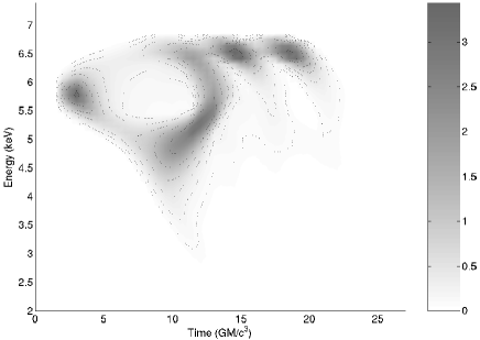
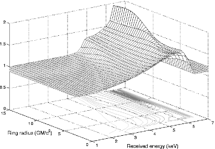
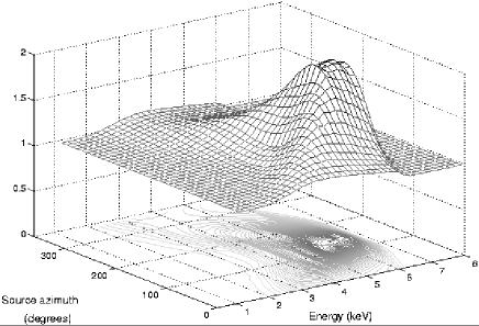
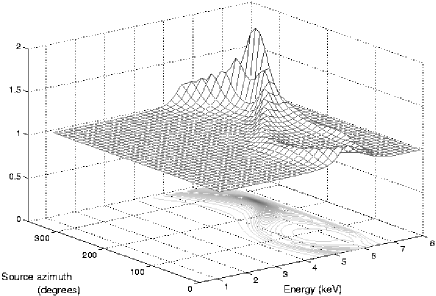
Figure 1: (a) Time-dependent spectrum produced by four flares: three simultaneous events at $(\rho_{s},\phi_{s})=(19\,r_{g},0^{\circ}),(10\,r_{g},100^{\circ}),(19\,r_{g},240^{\circ})$ followed by a repeat of the latter flare 4$\,t_{g}(=GM/c^{3})$ afterwards. (b) The full ‘1-d’ transfer function for time-averaged line profiles, generated from azimuthally averaged emissivity distributions corresponding to the ring-shaped flares swept out by orbiting flares. (c) Time-averaged spectra for a flare at $\rho_{s}=1.5\,r_{g}$ for each of the 36 azimuthal bins in the ‘2-d’ transfer function. (d) Same as (c) but for $\rho_{s}=10r_{g}$.

By following the procedure outlined in the previous section, we can generate the time-dependent spectrum produced by a single flaring event at a given location in spacetime. We can now obtain the transfer function $\mathcal{R}$ which maps the coordinates of an arbitrary number of flaring events to the data D. If the corona itself is optically thin (so that it has a negligible effect on the iron line emission), then we can simply superpose the spectrum coming from each individual flare, accounting for the time delays due to both the different source positions and the different time at which each flare becomes active. In this way, the transfer function becomes linear, although this is not a requirement for the inversion algorithm to work.

In this work we concentrate on the radial and azimuthal locations of the sources rather than their heights. Rather, we fix the height at a value which corresponds to a characteristic scale height of the corona which in practice is set to 2 or 5$\,r_{g}$, although it would be simple to extend these models to include the heights of the flares as well. The time lag arising from a difference in the $t_{s}$ coordinate of the source is handled trivially by simply shifting the total spectrum obtained from a single flare along the time axis by an appropriate amount. The delays coming from different values of $\rho_{s}$ and $\phi_{s}$ are handled by finding the earliest time at which photons from a particular source arrive at the observer for each source position. The entire spectrum is then shifted by this amount in the full transfer function. Figure 1 shows the resulting spectrum when the transfer function acts on a set of four flares, the coordinates of which are given in the caption. These spectra show the same qualitative features as those in the work of Reynolds et al. (1999), who gave the first examples of such time-dependent spectra.

While the aim of this paper is to present an inversion method for reverberation maps, data of this nature is not yet available. Rather, the best example of a broad iron line to date, seen in MCG–6-30-15, requires integration times so long that only basic variability analyses are viable (Iwasawa et al., 1999; Vaughan & Edelson, 2001; Shih et al., 2002). In this case to get a mean error of $\sim 15\%$, observations of hundreds of kiloseconds have been necessary (Fabian et al., 2002). A recent estimate of the mass of MCG–6-30-15 gives an upper limit of $\sim 10^{7}M_{\odot}$ (Morales & Fabian, 2002), corresponding to a characteristic time-scale ($GM/c^{3}$) of 49 seconds. For radii in the range $\sim 2-15$, Equation 13 implies orbit time-scales of less than one hour, which means that observations made with current telescopes such as XMM-Newton and Chandra span many orbital periods. This clearly calls for a modification of the technique as stated above, which we can accomplish by integrating over both $t_{s}$ and $\phi_{s}$ to yield a time-averaged spectrum for each radius of a flare, modelled as the ring it sweeps out over time, assuming it persists for an entire orbit. In practice, we can average the emissivity $F_{out}(r,\phi)$ over $\phi$ to obtain an axisymmetric profile and use a single time bin extending over the full duration of flux detection. In this case we can plot the entire transfer function, as shown in Figure 1.

In reality, of course, we do not expect a perfectly axisymmetric system, due to the turbulent and non-linear nature of the disc and corona. To begin to probe these effects one can imagine an intermediate scenario, where a time-averaged spectrum is obtained over an interval much shorter than the orbit time for a flare, or one where flaring events occur in ‘flashes’ which persist for times much less than the orbital period. In this case, we lose all the temporal information in the system but we can retain the azimuthal positions of the sources. The transfer function then consists of a time-averaged spectrum for each value of the pair $\rho_{s},\phi_{s}$ taken by a flare. In Figure 1 we show spectra for a source at a small radius $\rho_{s}=2$, for all values of $\phi$. Figure 1 shows the equivalent plot for a larger value of $\rho_{s}$. Averaging the spectra from these graphs over $\phi_{s}$ would produce cross-sections of Figure 1 at the corresponding radii.

4 Computational method

The eventual goal of this work is to construct a framework for determining patterns of coronal flaring activity from iron K$\alpha$ line spectra. We can assess the validity of conclusions drawn within this framework by testing the technique with data generated from a known distribution of flares. We operate on this distribution (known as the ‘truth’) with the transfer function $\mathcal{R}$ to yield the ‘mock data’ $\mathcal{R}\left({\tilde{\hbox{\bf\em h}}}\right)$. To complete the process we add a known amount of Gaussian noise $\sigma$, to obtain the simulated data $\hbox{\bf\em D}=\mathcal{R}\left({\tilde{\hbox{\bf\em h}}}\right)+\sigma$.

Figure 2: A schematic representation of the process by which we test the technique

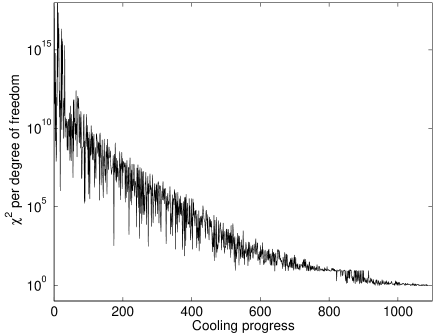
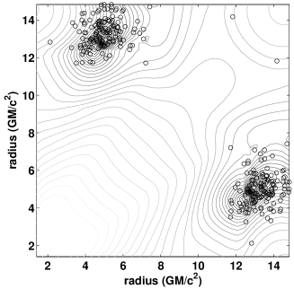
Figure 3: (a) The $\chi^{2}$ statistic (per degree of freedom) for simulated data compared with the mock data produced by operating with the transfer function on the mean of the sampled posterior. As the algorithm progresses, it can be seen to converge toward the true posterior, arriving at a $\chi^{2}$ of $48.8/50$. (b) A snapshot of some of the final samples. The true posterior is shown as the contour plot and the small circles represent the samples, showing that they are concentrated in regions of maximum posterior probability. The diagonal reflection symmetry is due to the flares being indistinguishable.

Given these simulated data we can construct an inference h via the Massive Inference method, which can then be compared with the truth ${\tilde{\hbox{\bf\em h}}}$. A graphical summary of this process is shown in Figure 2.

Sampling of the posterior is achieved with a Markov Chain Monte Carlo algorithm, using a simulated annealing cooling schedule. Each consecutive sample is chosen according to a ‘temperature’ parameter, which is increasingly restrictive in terms of the changes it allows as the system cools. The samples are initially spread over a large region of parameter space, but as the temperature drops, they become more concentrated around regions of high posterior probability. The algorithm can store an ensemble of several flare configurations, each evolving independently, and the system is cooled as slowly as computation time allows. In this way, we maximise the number of samples taken and minimise the chance that the samples are trapped within local minima.

There is no formal convergence test for the Massive Inference method. Rather, one can vary both the rate at which the algorithm anneals and the size of the ensemble of simultaneously evolving parameter sets, and check that they all converge to a single distribution. A representation of convergence for a simple example involving only two flares is shown in Figure 3. The flares are located at radii of 5 and 13 $r_{g}$. Figure 3 shows the misfit between the mock and simulated data as the algorithm progresses from its initial, hot state to the final cool state. The decrease in temperature is visible as the tapering of the curve’s overall envelope of variation, while the convergence is reflected in the approach of $\chi^{2}$ (per degree of freedom) toward the final value of $48.8/50$. In Figure 3 we plot a projection of the sampled posterior into a plane showing the radial coordinate of each flare, together with a contour plot of the true posterior, showing that the samples are indeed concentrated around its peak.

5 Time-dependent inversions

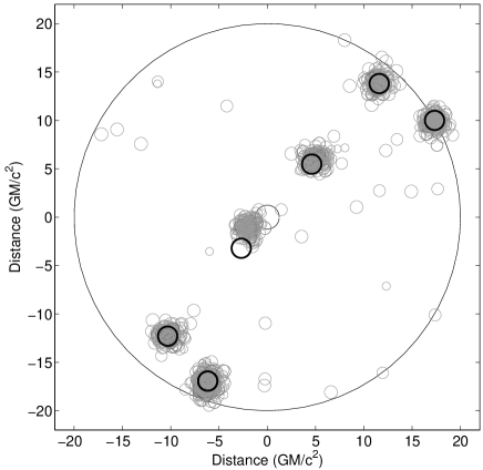
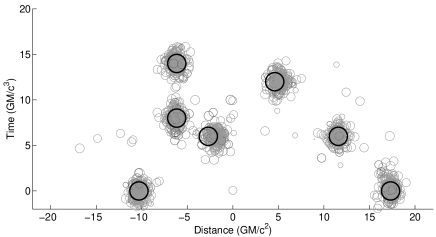
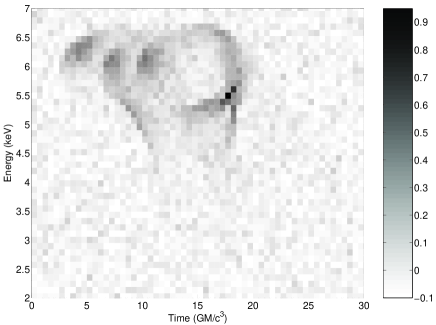
Figure 4: (a) Samples from the posterior probability distribution for a configuration of 7 flares, projected into the equatorial plane. Only 6 flares are visible because two are located above the same point in the disc, but are separated in time. The largest circle marks the edge of the polar grid of allowed positions, not the edge of the accretion disc. (b) The same samples, but now projected into the $t$-$x$ plane. The observer is located above the negative $y$ axis, nearest the bottom of (a). (c) The simulated noisy data from which the inference was made, with a mean SNR = 1. (d) A histogram showing the inferred number of flares, $N$.

We now present some examples of the application of our technique to simulated reverberation maps, obtained by adding noise to spectra such as that shown in Figure 1. We quote noise levels as mean signal-to-noise ratios (SNR), the ratio of the noise to the average over all pixels in which the flux is non-zero. For a particular example of simulated data with a mean SNR of 1, which we take as our starting point for illustrating the technique, the inferred number of flares is given in Figure 4, where a strong peak is visible at the true number of 7. The locations of the flare ensemble above the accretion disc (their $\rho_{s},\phi_{s}$ coordinates) are shown in Figure 4, where each sample of the posterior is plotted as a set of $N$ grey circles, where $N$ is the number of flares corresponding to that particular sample. In reality, the inner 20$\,r_{g}$ of the disc are covered by a 20 radii $\times$ 18 azimuths polar grid of flare positions, but to help visualise the results, we have displaced each grey circle in a random direction from the centre of its grid cell by a radius obtained by sampling from a Gaussian distribution with a standard deviation equal to the radius of the thicker, black circles, whose centres mark the location of each flare in the true configuration. The radius of each grey circle is proportional to the strength of the flare for that sample and is normalised such that the strongest flare’s radius matches that of the thicker circles marking the truth.

In addition, we plot two circles centred on the origin, which mark the inner radius of the accretion disc and the radius $\rho_{s}=20\,r_{g}$ which corresponds to the outer limit of the polar grid, but not the accretion disc itself ($r_{max}=100\,r_{g}$). The samples are clustered around the true positions in all cases but one, showing that the system copes well with a problem of this complexity, at this level of noise in the data. Figure 4 shows the inferred distribution of times at which each flaring event occurred, as a projection onto the $t$-$x$ plane (the observer is located above the negative $y$ axis, nearest the bottom of the plot). For the flare closest to the black hole whose $x$-$y$ position was least accurately inferred, the samples’ time coordinates are centred around the true value of 6 $t_{g}$. It is very difficult to pick out 7 distinct spectra by eye in the simulated data shown in Figure 4, and yet the algorithm is able to do so, and give the locations of the flares with a good degree of accuracy.

We show two more examples in Figures 5 and 6, one for a configuration of 11 flares and a mean SNR = 2, and one for poorer quality data (SNR = 0.5) with fewer flares in the truth. Figure 5 shows a 3-d representation of the locations in spacetime of the true and inferred distributions of flaring events. The vertical axis measures time, not the height of the flares, which is fixed at 5$\,r_{g}$. The light grey samples on the disc and at the side of the plot correspond to the $x$-$y$ and $t$-$x$ projections like those shown in Figures 4 and 4 for the case of seven flares. The truth is plotted here as a set of wire-frame cubes with a side length equal to twice the standard deviation of the Gaussian distribution from which the amount of radial displacement of each dark grey sample was taken.

The noisy data and a histogram of the inferred number of flares are shown in Figures 5 and 5. It is clear that at least 11 flares were chosen each time in order to fit the data and higher numbers become increasingly unlikely, reflecting the prior probability distribution on $N$. Information from Figures 5 and 5 can be combined by plotting the latter in colour. Instead of grey circles, we can use a different colour for each value of $N$ in the histogram. We avoid certain colours being obscured by others plotted over the top by randomising the order in which they are drawn, thus giving a visual impression of the histogram, which can be useful in revealing spatial bias of different values of $N$. Colour versions of all relevant plots in this paper are available online.

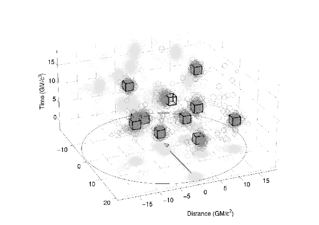
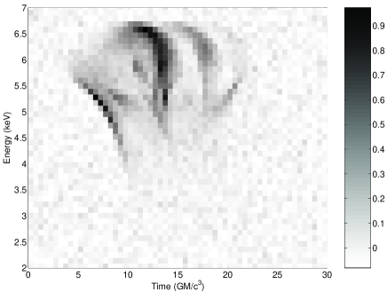
Figure 5: (a) Samples from a posterior distribution corresponding to a truth consisting of 11 flares, shown as wire-frame cubes. The time at which each flare became active is plotted along the vertical axis. The height of each flare is fixed at $h_{s}$ = 5$\,r_{g}$. The lighter circles plotted on the equatorial plane and the vertical plane at the back of the plot correspond to the two projections of Figures 4 and 4 for the case of 7 flares. (b) Simulated reverberation map from which this inference was made, at a mean SNR = 2. (c) A histogram showing the distribution of values of $N$, the number of flares, chosen by the algorithm during sampling.

Figure 6 shows an inversion performed for data at a higher noise level (mean SNR = 0.5). In both 3-d plots, the thick arrow drawn in the plane of the disc is directed towards the observer.

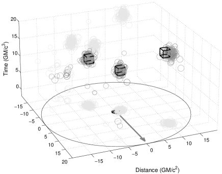
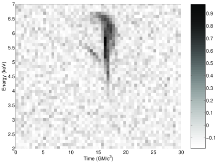
Figure 6: (a) Samples from the posterior distribution for a truth with 3 flares, made at a higher level of noise (mean SNR = 0.5) in the simulated data, shown in (b). For this inference, the histogram for $N$ (not shown) shows a single dominant peak at the correct number of 3 flares.

As the level of noise is increased, the quality of the inferences decreases – flares begin to be missed or show up in incorrect places. Rather than perform a detailed analysis of the limits of performance of the above time-dependent setup, we now consider those of time-averaged spectra, where we focus on just the $\rho_{s}$ and $\phi_{s}$ coordinates of the flares. The reason for this two-fold. Firstly, the behaviour of the system for demanding noise levels in time-averaged data is a scenario more likely to be of interest in the short to medium term, given the quality of current data. Secondly, obtaining the locations of a set of flares in time is a relatively easy problem compared to that of revealing their spatial locations, simply because the structure induced in the data for a single flare at different times is far more distinctive than at different positions. It was described in Section 3.1 that the former is achieved by simply translating the spectrum from one flare along the time axis in the data-space by an amount corresponding to its time-delay, whereas the spectral differences that come from changes in spatial location are far more subtle. It is therefore clearer to focus on the time-averaged scenarios described in the next section.

6 Time-averaged inversions

We can recast the above system in a form which does not depend on time by summing the spectra over their entire duration, and removing all reference to time from the transfer function. In this way, we obtain a 2-dimensional problem, where we aim to recover the $\rho_{s}$ and $\phi_{s}$ coordinates of each source, which take values in the range 1.5 – 15$\,r_{g}$ and 0 – 360^∘ over a grid of 40 radii $\times$ 36 azimuths. In doing this, we have reduced the number of degrees of freedom (d.o.f.) in the data by almost two orders of magnitude, and as a result we readily find noise levels at which the system struggles to produce correct inferences.

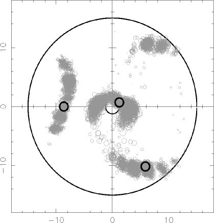
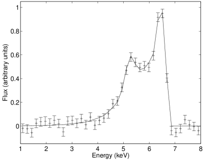
Figure 7: (a) Posterior samples for a distribution of 3 flares, inferred from time-averaged data, hence only an equatorial plane projection is available. The true flare positions are marked with thick circles and the large circle at 15$\,r_{g}$ marks the outer limit of allowed flare positions. (b) The time-averaged spectral line used in this reconstruction, shown as the points with error-bars. The mean signal-to-noise ratio was 7, corresponding to an average noise level of $\sim 15\%$. The solid line shows the mock data from the inference. (c) A histogram for the value of $N$ corresponding to each set of samples shown in (a). Although the samples are clustered around four distinct regions, the algorithm rarely picked sets of four flares, instead preferring the correct number of three.

Figure 7 shows the set of samples of the posterior probability distribution for an inference based on the data of Figure 7. The true distribution contains three flares at the locations shown by the thick black circles in Figure 7. In addition to being spread out over many cells of the polar grid of different $\rho_{s},\phi_{s}$ values, the inference is also clustered around a region above the rear, receding part of the disc, in which there is no flare in the truth. The mock data do provide a satisfactory fit to the simulated data, however, which implies that, at this level of noise, we are probing degenerate regions of the transfer function. We note further that the samples of $N$ shown in Figure 7 peak very strongly at the true number of three, so that the extra cluster of samples in Figure 7 does not imply the presence of a fourth flare, rather an additional possibility for the location of one of the three.

6.1 Linear-dependence in the transfer function

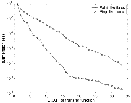
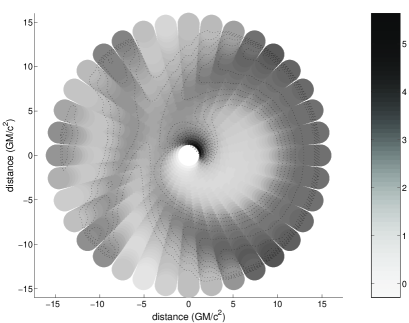
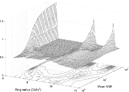
Figure 8: (a) Singular values of the time-averaged transfer functions, for the 2-d system (inferring $\rho_{s}$ and $\phi_{s}$) shown as squares and the 1-d system (inferring just $\rho_{s}$) shown as circles. Losing azimuthal information results in a dramatic reduction in the transfer function’s linear independence. (b) The average of the flare-space singular vectors for the 2-d system, showing degenerate regions above the accretion disc, within which a flare produces very similar features in the data. On the approach (left-hand) side of the disc, beaming produces sharper structure in the data which leads to smaller degenerate regions and a greater spatial accuracy. (c) Inferred (ring-shaped) flare radii and strengths for 3 flares at different levels of noise, plotted as the mean flare strength in each of the 40 radial bins. At SNR = 10, two flaring regions are revealed, but a further factor 10 reduction in the noise is necessary in order to successfully resolve the 3 flares.

We can quantify the linear-dependence present in the transfer function by performing a singular value decomposition, yielding the singular values marked by the squares in Figure 8. The gradient of this line determines the decrease in noise that is necessary, on average, in order to detect the presence of extra flares as they are added into the true distribution. The ‘flare-space’ singular vectors (in the space of all possible flare configurations) always form a linearly-independent basis, with which we can represent any flare pattern. However, their relative magnitudes are given by the singular values, which means that for a given finite noise level, a certain (large) fraction are effectively zero, removing this ability to span flare-space and represent an arbitrary pattern. Degenerate regions arise when the projection of some of a particular flare pattern lies in these zero directions and fails to result in detectable features in the data.

A useful measure of the overall effect of this is shown in Figure 8, where we have summed each singular vector, weighted by the singular values, and projected the result onto the polar grid covering the inner regions of the accretions disc. A grey circle is drawn at the centre of each grid cell, whose shading gives the overlap of the average singular vector with the cell. The radii of the circles increase linearly with radius to provide a suitable covering of the disc, for ease of visualisation only. The plot reveals those cells which, on average, produce the same type of structure in the data and which require higher levels of noise to distinguish between them. This explains the patterns seen in the inferred flare locations shown in Figure 7 as the algorithm explores the contours of Figure 8 with approximately equal frequency, in its search to fit the data. This plot also reveals the effective spatial resolution of the technique, as a function of position on the disc. Two adjacent flares placed in cells corresponding to a high gradient in Figure 8 will be easier to resolve than two placed in a region where the gradient is small.

As described in Section 3.1, we can reduce the level of complexity in the transfer function still further by calculating the time-averaged spectra which arise from axisymmetric distributions of emissivity due to ‘ring-shaped’ flares, modelling time-averaged point-like flares which persist over an entire orbit or more. We generate these axisymmetric emissivity profiles by averaging the illumination pattern due to a single flare over all values of $\phi_{s}$, resulting in a 1-d problem where we attempt to recover just the radius $\rho_{s}$ of the ring.

Performing this procedure results in a transfer function whose singular values are given by the circles in Figure 8. They drop much more quickly than for the 2-d version, giving a difference of one order of magnitude for just 5 flares. This trend is reflected in the picture of the 1-d transfer function shown in Figure 1, where the line profile shows only modest variation as a function of radius. To illustrate the difficulty in performing inference calculations with this system, we show the results of many such calculations for a wide range of noise, in Figure 8, where we plot the mean strength of the samples in each radial bin. At high noise levels (SNR $\sim$ 1) none of the three flares present in the truth was located in the inference. For noise levels comparable to the 2-d calculation of Figure 7, the innermost flare was detected, but it required a further drop of about a factor of 10 in noise before all three flares could be detected.

7 Application to MCG–6-30-15

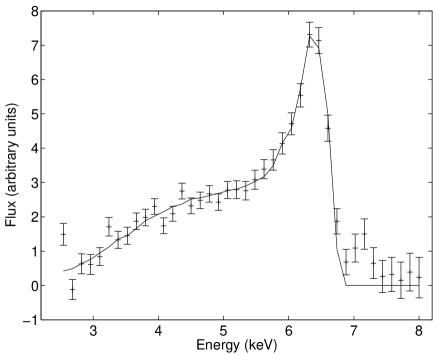
Figure 9: (a) Inferred distribution of samples for the XMM-Newton data shown as the error-bars in (b). (b) The solid line shows the mock data obtained by operating on the inferred flare distribution with the transfer function, together with the data themselves.

We now apply the technique to the results of a 325 ks observation of MCG–6-30-15 made with XMM-Newton, described fully in Fabian et al. (2002). We take the spectral line to be the difference between their Model 4 for the underlying continuum, and the data. The average noise level is approximately 15%, which corresponds to a mean SNR $\sim$ 7. Given the results of Figure 8, it seems highly doubtful that any meaningful inferences can be made within the 1-d axisymmetric, time-averaged framework at the level of noise. We choose instead to apply the 2-d system, but with the following large caveat. Recent estimates of the mass of MCG–6-30-15 give values close to $10^{7}M_{\odot}$ giving a characteristic time-scale of 49 seconds, which, as discussed in Section 3.1, corresponds to an orbital period of less than one hour even for a relatively slow flare, orbiting at $\rho_{s}=15\,r_{g}$.

It is clear from these time-scales that we cannot hope to attribute structure in the line profile to particular non-axisymmetric features in the results of any inference calculation, although such results may be useful in giving an indication of the general radii at which flares could be active. In addition, we make no attempt in this work to model the form of the underlying continuum spectrum, and so are completely reliant on such a model to define a given spectral line shape. Models for the continuum, while providing a good overall fit, still allow considerable variation of the slope in the vicinity of the iron line, thus altering the shape. Detailed predictions of flaring activity based on the precise details of this line profile can therefore be easily changed with a different continuum model, and should not be taken as clear evidence of a particular flare distribution. This paper is intended to demonstrate the type of calculation which will become possible with the advent of high quality, time-dependent spectral data. The application of our techniques to this XMM-Newton observation is a check, to make sure we obtain a plausible picture from current data which is consistent with previous studies of this object.

Figure 9 shows the results of applying the 2-d system to these data. The posterior samples are concentrated in two regions, and the histogram for the number of flares (not shown) has a very strong peak at $N=2$. The solid line in Figure 9 shows the mock data from this inferred flare pattern, which provides a good fit with the data below $\sim 7$ keV. The structure above $\sim 7$ keV is due to iron K$\beta$ emission (Fabian et al., 2002), which we do not include in our transfer function (although it would be simple to do so). For this reason, we ignore the points above 7 keV when calculating the value of $\chi^{2}$ for this fit, which is 0.98 per degree of freedom. That the flaring regions are contained within a few gravitational radii of the central black hole, which leads to a very steep emissivity profile in this region, is consistent with the existing picture of this object based on previous studies.

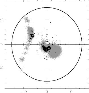
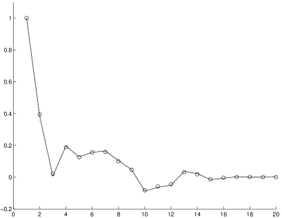
Figure 10: (a) Samples from the results of applying the 2-d system to noisy data generated from a truth consisting of the results of Figure 9, using a noise level equivalent to that in the XMM-Newton data. (b) Same as (a) except for a different random seed used to generate the data. (c) The data themselves. The squares show the data used to obtain (a) and the circles (b), with the error-bars omitted for clarity. The solid line shows the mock data from the results in (a) and the dashed line for (b). (c) The projection of the truth (ie the results of Figure 9) onto the first twenty singular vectors, shown as the solid line. The remaining coefficients are negligible. The circles show a similar projection for the inference in (a) and the dotted line shows the projection of the inference in (b).

Whether the precise azimuthal distribution of flares has a direct physical significance, given the time-scales involved, is doubtful. However, it is important to assess the uniqueness of this prediction – to what extent would the result change with a different realisation of the noise in the data? To address this issue, we can perform a further simulation based on the results of Figure 9 as follows. By taking a truth consisting of the mean flare-strength in each grid cell, we can generate mock data to which we add an amount of noise corresponding to that in the original data in Figure 9. We can then perform repeated applications of the inversion technique for different random seeds in our noise generator. Figure 10 shows the results of two such calculations. The thick circles show the ‘truth’ consisting of the results of Figure 9, and the grey circles show the samples of the posterior probability. In Figure 10 we obtain very similar results to the original inference, but in Figure 10 we see some differences. Again, we can interpret this result within the singular vectors of Figure 8 – the ‘erroneous’ samples are continuously connected along regions of high degeneracy. For this reason, we should interpret the results of Figure 9 as indicating the presence of flares anywhere within the two regions in Figure 10. Figure 10 shows the noisy data for the two different realisations of noise and the solid and dashed lines are the mock data corresponding to Figures 10 and 10 respectively. Another way of seeing how similar the two different flaring patterns are, when considered in the context of the singular vectors, is to evaluate the components of the two patterns on the singular vector basis. The solid line in Figure 10 gives the projection of the ‘real’ results of Figure 9 onto the singular vectors, and the circles and dotted line correspond to those for Figures 10 and 10 respectively. It is through projections like these that we can assess the true similarity of structure in the data that different patterns of flaring activity can produce.

8 Conclusion

We have presented a new way of analysing line profile data which constrains the number, positions and strengths of hard X-ray sources in an accretion disc’s corona. The method makes use of the ‘Massive Inference’ prior probability distribution which is based on an assumption of discrete, point-like sources.

By applying it to simulated noisy reverberation maps, we found that the technique performs well, making the most of the rich information content of such data. The algorithm was able to disentangle the complicated signatures of combinations of flare events, rather than concentrating on scenarios where it can be assumed that one or two dominant flares are responsible for the observed data (Reynolds et al., 1999; Young & Reynolds, 2000). Indeed, if there is only a single large flare present, such a conclusion will be reached by our method.

Reverberation mapping of relativistic spectral lines is still some way off, and so we modified our system to treat time-averaged spectra at similar levels of noise to those obtained by current instruments such as XMM-Newton and Chandra. In doing so we lost all the temporal information in the transfer function and reduced the problem to that of inferring the set of radial and azimuthal coordinates of the flares. The relative information loss in the data, however, was greater than in the parameter space, and the resulting inference problem was more challenging. At realistic levels of noise, we found some ambiguity in the inferred spatial locations of the flare, but less in the inferred number present in the ensemble. This ambiguity was quantified using a singular value decomposition, which yielded a ‘map’ of the disc showing the relative ease with which different regions of the disc could be differentiated, and gave a limit on the spatial resolution of the technique.

We reduced the problem still further, considering data collected on time-scales greater than the orbital period of each flare. In this case we averaged the illumination pattern of a flare over the azimuthal coordinate $\phi_{s}$ to obtain a 1-d transfer function based on ‘ring-like’ sources, and attempted to constrain the radii of these rings. This problem proved to be very difficult, requiring very low levels of noise to obtain useful results. This very high level of degeneracy in the transfer function is due to the line profile being affected only weakly by the position of the source, the dominant contribution coming from the relativistic effects occurring during the photons’ subsequent journey from disc to observer.

As a consistency check, we applied the technique to a recent observation of the iron K$\alpha$ line in MCG–6-30-15 made by XMM-Newton over 325 ks. This long integration time means that, given the mass of the central black hole of $\sim 10^{7}M_{\odot}$, it is not possible to resolve any structure in the data due to non-axisymmetric illumination of the disc, and that the 1-d ring-based transfer function is most appropriate. However, given the difficulties present in the highly degenerate ring-based system described above, we applied the 2-d time-averaged algorithm to this data, allowing some azimuthal structure in the corona. We found two regions of flaring activity, one at a radius of $\sim 2\,r_{g}$ on the near side of the disc which is responsible for the bulk of the highly redshifted emission below 5 keV, and one on the approaching side at $\sim 6\,r_{g}$ which is more beamed and produces the tall peak close to 6.4 keV.

Further simulations for different realisations of random noise illustrated explicitly that this result must be interpreted with the singular vector map of Figure 8 in mind, spreading out the regions occupied by the samples to cover those in Figure 10. This approach showed that, within the assumptions underlying the method (mainly that different locations of X-ray flares in the strong-gravity region of the central black hole account for structure in the line profile), the results of Figure 9 are quite robust. Physically, however, we should not expect to be able to pick out any particular azimuthal region based on a 325 ks observation. In fact, by including a relatively weak, narrow component in the line in order to account for the tall peak near 6.4 keV, it is possible to achieve a very good fit with the data based on an azimuthally averaged illumination pattern (Miniutti et al., 2003). In addition, the uncertainty that comes from defining a spectral line shape relative to a given model for the underlying continuum radiation, means that the above results (other than the loose condition that the flares are contained within $\sim 15\,r_{g}$) can be changed very easily by making different assumptions about the continuum. For these reasons, we do not claim that the results of Figure 9 are a meaningful prediction for MCG–6-30-15, rather, it is reassuring to obtain a pattern contained within a few gravitational radii of the central black hole, and gives an indication of the sort of results which may become viable with higher quality data. It is with the advent of high-quality, time-dependent spectral data, like that promised by missions such as Constellation-X, that inversion techniques such as those described here offer the possibility of mapping the hard X-ray emission within a few gravitational radii of a black hole.

Appendix A Geodesic motion

The gravitational calculations in this paper were performed using geometric algebra, within a new formulation of gravity theory recently developed by Lasenby et al. (1998). In this appendix we translate some of the results of these calculations into conventional notation, but mention only in passing the motivation for casting the problem in this form. For a detailed account of the tools and ideas which lead to these results, see Lasenby et al. (1998), Hestenes (1966) and Hestenes & Sobczyk (1984).

We begin with an orthonormal tetrad with components on the Boyer-Lindquist coordinate frame given by

$$\hat{t}=\frac{r^{2}+a^{2}}{\rho\sqrt{\Delta}}\,\partial_{t}+\frac{a}{\rho\sqrt{\Delta}}\,\partial_{\phi}\qquad\quad\hat{r}=\frac{\sqrt{\Delta}}{\rho}\,\partial_{r}\qquad\quad\hat{\theta}=\frac{1}{\rho}\,\partial_{\theta}\qquad\quad\hat{\phi}=\frac{a\sin\theta}{\rho}\,\partial_{t}+\frac{1}{\rho\sin\theta}\,\partial_{\phi}$$ (21)

where

$$\rho^{2}=r^{2}+a^{2}\cos^{2}\theta,\qquad\Delta=r^{2}+a^{2}-2r.$$ (22)

We can then parametrise a photon’s momentum with the direction-cosines $\alpha$ and $\beta$ and the energy parameter $\Phi$ as follows

$$p=\Phi\,\left(\hat{t}+\cos\alpha\cos\beta\,\hat{r}-\sin\alpha\cos\beta\,\hat{\theta}+\sin\beta\,\hat{\phi}\right).$$ (23)

This form is based on the (principal) null vector $\hat{t}+\hat{r}$, on which we perform two orthogonal rotations by the angles $\alpha$ and $\beta$. In this way, the vanishing norm of the vector is built into its parametrisation, removing a degree of freedom from the calculation from the outset. In addition, we obtain a simple picture of the momentum vector in terms of rotors (see e.g. Lasenby et al. (1998)). This form of $p$ yields the following first derivatives of the coordinates $x^{\mu}$:

$$\dot{t}=\frac{\Phi}{\rho\sqrt{\Delta}}\left(a\sin\theta\sin\beta\sqrt{\Delta}+r^{2}+a^{2}\right)\qquad\dot{r}=\frac{\Phi\sqrt{\Delta}}{\rho}\,\cos\alpha\cos\beta\qquad\dot{\theta}=-\frac{\Phi}{\rho}\sin\alpha\cos\beta\qquad\dot{\phi}=\frac{\Phi}{\rho}\left(\frac{a}{\sqrt{\Delta}}+\frac{\sin\beta}{\sin\theta}\right)$$ (24)

Substituting $p$ into the geodesic equation results in the following expressions for $\dot{\Phi}$, $\dot{\alpha}$ and $\dot{\beta}$:

$$\dot{\Phi} = \frac{-\Phi^{2}\cos\beta}{2\rho^{3}}\Bigg{[}a^{2}\sin 2\theta\,\sin\alpha+\left(-4ra\sin\theta\,\sin\beta+\frac{\rho^{2}(r^{2}-a^{2})}{r\sqrt{\Delta}}+\sqrt{\Delta}\left(\rho^{2}-2r^{2}\right)\right)\cos\alpha\Bigg{]}$$ (25)

$$\dot{\alpha} = \frac{\Phi}{\rho^{3}\cos\beta}\Bigg{[}\sin\alpha\bigg{(}\frac{1}{2r\sqrt{\Delta}}\left(\Delta(\rho^{2}-4r^{2})+\rho^{2}(r^{2}-a^{2})\right)-2ra\sin\theta\sin\beta\bigg{)}$$ (26)

$$\phantom{\frac{\Phi}{\rho^{3}\cos\beta}[]}\quad-\cos\theta\cos\alpha\sin\beta\bigg{(}2a\sqrt{\Delta}+\frac{\sin\beta}{\sin\theta}\left(2(r^{2}+a^{2})-\rho^{2}\right)\bigg{)}\Bigg{]}$$

$$\dot{\beta} = \frac{\Phi}{\rho^{3}}\Bigg{[}\cos\theta\sin\alpha\left(2a\sqrt{\Delta}+\frac{\left(r^{2}+a^{2}\right)+a^{2}\sin^{2}\theta}{\sin\theta}\sin\beta\right)$$ (27)

$$\phantom{\frac{\Phi}{\rho^{3}}[]}\quad-\cos\alpha\sin\beta\left(\frac{r\left(\Delta+a^{2}\sin^{2}\theta\right)-m\left(r^{2}-a^{2}\cos^{2}\theta\right)}{\sqrt{\Delta}}\right)+2ra\sin\theta\sin\beta\Bigg{]}$$

These equations complete a first order set of 7 equations for the coordinates $\{t,r,\theta,\phi\}$ and the parameters $\Phi$, $\alpha$ and $\beta$, which is sufficient to determine photon’s trajectory and is numerically very stable. A further advantage of this approach is that we have not yet made any use of the three conserved Killing quantities; the energy $E$, angular momentum $J$ and Carter constant $Q$. In terms of spacetime position and our three photon momentum parameters, they are given by

$$E=\frac{\Phi}{\rho}(\sqrt{\Delta}+a\sin\theta\sin\beta)\qquad J=\frac{\Phi}{\rho}\left(\sqrt{\Delta}a\sin^{2}\theta+\sin\theta\sin\beta\left(r^{2}+a^{2}\right)\right)\qquad Q=\Phi^{2}\rho^{2}\left(1-\cos^{2}\alpha\cos^{2}\beta\right).$$ (28)

By evaluating these quantities explicitly at various points along a photon trajectory we can test that the integration is proceeding correctly.

We apply the same basic idea to calculate the circular, timelike trajectories in the equatorial plane which model the flow of accreting matter, except now we can use a single parameter $U$, as follows:

$$v=\cosh U\hat{t}+\sinh U\hat{\phi}$$ (29)

where the geodesic equations are satisfied by

$$\tanh U=\frac{\sqrt{r}-a}{\sqrt{\Delta}}.$$ (30)

More commonly, these trajectories are written as

$$v\propto\partial_{t}+\Omega\,\partial_{\phi},\qquad\Omega=\frac{1}{a+r^{3/2}}$$ (31)

and the constant of proportionality is obtained by imposing the condition $v^{2}=1$. The two notations are related via

$$\Omega=\frac{a+\tanh U\sqrt{\Delta}}{r^{2}+a^{2}+\tanh U\>a\sqrt{\Delta}}.$$ (32)

In order to model the motion of a source orbiting with the disk matter, but at a general height $h_{s}=r\sin\theta$ above the equatorial plane, we can define a trajectory (no longer geodesic) as follows

$$v_{s}\propto\partial_{t}+\Omega\,\partial_{\phi},\qquad\Omega=\frac{1}{a+(r\sin\theta)^{3/2}},$$ (33)

effectively lifting a circular geodesic vertically out of the equatorial plane. The expression for $U$ given by Equation (30) generalises to

$$\tanh U=\frac{r^{2}-a(r\sin\theta)^{3/2}}{a\cos^{2}\theta+(r\sin\theta)^{3/2}}\,\frac{\sin\theta}{\sqrt{\Delta}}$$ (34)

In order to measure the angle at which a photon leaves the source and hits the disk we must define a co-moving 3-frame attached to $v_{s}$ ($v$ being a special case where $\theta=\pi/2$. Together with Equation (29), the vectors $\hat{r}$, $\hat{\theta}$ and $\hat{\phi}^{\prime}$, where

$$\hat{\phi}^{\prime}=\sinh U\hat{\phi}+\cosh U\hat{t},$$ (35)

form a convenient orthonormal tetrad.

References

- Dabrowski et al. (1997) Dabrowski Y., Fabian A. C., Iwasawa K., Lasenby A. N., Reynolds C. S., 1997, MNRAS, 288, L11
- Fabian et al. (1995) Fabian A. C., Nandra K., Reynolds C. S., Brandt W. N., Otani C., Tanaka Y., Inoue H., Iwasawa K., 1995, MNRAS, 277, L11
- Fabian & Vaughan (2003) Fabian A. C., Vaughan S., 2003, MNRAS, 340, L28
- Fabian et al. (2002) Fabian A. C., Vaughan S., Nandra K., Iwasawa K., Ballantyne D. R., Lee J. C., De Rosa A., Turner A., Young A. J., 2002, MNRAS, 335, L1
- George & Fabian (1991) George I. M., Fabian A. C., 1991, MNRAS, 249, 352
- Gull (1989) Gull S., 1989, Developments in Maximum Entropy data analysis. J.Skilling (ed), Kluwer Academic Publishers, Dordtrecht
- Gull & Daniell (1978) Gull S. F., Daniell G. J., 1978, Nature, 272, 686
- Hestenes (1966) Hestenes D., 1966, Space-Time Algebra. Gordon and Breach, New York
- Hestenes & Sobczyk (1984) Hestenes D., Sobczyk G., 1984, Clifford Algebra to Geometric Calculus. Reidel, Dordrecht
- Iwasawa et al. (1996) Iwasawa K., Fabian A. C., Reynolds C. S., Nandra K., Otani C., Inoue H., Hayashida K., Brandt W. N., Dotani T., Kunieda H., Matsuoka M., Tanaka Y., 1996, MNRAS, 282, 1038
- Iwasawa et al. (1999) Iwasawa K., Fabian A. C., Young A. J., Inoue H., Matsumoto C., 1999, MNRAS, 306, L19
- Laor (1991) Laor A., 1991, ApJ, 376, 90
- Lasenby et al. (1998) Lasenby A., Doran C., Gull S., 1998, Phil. Trans. R. Soc. Lond. A, 356, 487
- Lu & Yu (2001) Lu Y., Yu Q., 2001, ApJ, 561, 660
- Martocchia et al. (2000) Martocchia A., Karas V., Matt G., 2000, MNRAS, 312, 817
- Matt et al. (1991) Matt G., Perola G. C., Piro L., 1991, A&A, 247, 25
- Miniutti et al. (2003) Miniutti G., Fabian A. C., Goyder R., Lasenby A. N., 2003, MNRAS, 344, L22
- Morales & Fabian (2002) Morales R., Fabian A. C., 2002, MNRAS, 329, 209
- Reynolds & Begelman (1997) Reynolds C. S., Begelman M. C., 1997, ApJ, 488, 109
- Reynolds et al. (1999) Reynolds C. S., Young A. J., Begelman M. C., Fabian A. C., 1999, ApJ, 514, 164
- Shih et al. (2002) Shih D. C., Iwasawa K., Fabian A. C., 2002, MNRAS, 333, 687
- Skilling (1998) Skilling J., 1998, Massive Inference and Maximum Entropy. Maximum Entropy and Bayesian Methods, Kluwer Academic Publishers, Dordtrecht
- Skilling (1999) Skilling J., 1999, MassInf Programmers’ Notes, http://www.maxent.co.uk
- Tanaka et al. (1995) Tanaka Y., Nandra K., Fabian A. C., Inoue H., Otani C., Dotani T., Hayashida K., Iwasawa K., Kii T., Kunieda H., Makino F., Matsuoka M., 1995, Nature, 375, 659
- Vaughan & Edelson (2001) Vaughan S., Edelson R., 2001, ApJ, 548, 694
- Wilms et al. (2001) Wilms J., Reynolds C. S., Begelman M. C., Reeves J., Molendi S., Staubert R., Kendziorra E., 2001, MNRAS, 328, L27
- Young & Reynolds (2000) Young A. J., Reynolds C. S., 2000, ApJ, 529, 101
- Young et al. (1998) Young A. J., Ross R. R., Fabian A. C., 1998, MNRAS, 300, L11