GENERATING EQUILIBRIUM DARK MATTER HALOS:
INADEQUACIES OF THE LOCAL MAXWELLIAN APPROXIMATION

Abstract

We describe an algorithm for constructing $N$-body realizations of equilibrium spherical systems. A general form for the mass density $\rho(r)$ is used, making it possible to represent most of the popular density profiles found in the literature, including the cuspy density profiles found in high-resolution cosmological simulations. We demonstrate explicitly that our models are in equilibrium. In contrast, many existing $N$-body realizations of isolated systems have been constructed under the assumption that the local velocity distribution is Maxwellian. We show that a Maxwellian halo with an initial $\rho(r)\propto r^{-1}$ central density cusp immediately develops a constant-density core. Moreover, after just one crossing time the orbital anisotropy has changed over the entire system, and the initially isotropic model becomes radially anisotropic. These effects have important implications for many studies, including the survival of substructure in cold dark matter (CDM) models. Comparing the evolution and mass-loss rate of isotropic Maxwellian and self-consistent Navarro, Frenk, & White (NFW) satellites orbiting inside a static host CDM potential, we find that the former are unrealistically susceptible to tidal disruption. Thus, recent studies of the mass-loss rate and disruption timescales of substructure in CDM models may be compromized by using the Maxwellian approximation. We also demonstrate that a radially anisotropic, self-consistent NFW satellite loses mass at a rate several times higher than that of its isotropic counterpart on the same external tidal field and orbit.

The Astrophysical Journal, accepted

1 INTRODUCTION

Despite the inexorable increase in the dynamic range of current cosmological $N$-body simulations, they still cannot address many questions regarding the detailed physical processes taking place inside galaxies. Examples include the survival and evolution of substructure within dark matter (DM) halos (Moore, Katz & Lake 1996; Taffoni et al. 2003; Hayashi et al. 2003), the effects of tidal stripping and dynamical friction on the orbits of satellites (Velázquez & White 1995; van den Bosch et al. 1999; Colpi, Mayer & Governato 1999; Mayer et al. 2002) and the consequent heating of galactic disks (Quinn & Goodman 1986; Velázquez & White 1999; Taylor & Babul 2001; Font et al. 2001), the susceptibility of disks to bar instabilities (Mihos, McGaugh & de Blok 1997), and the effects of these bars on halo central density cusps (Debattista & Sellwood 2000; Athanassoula 2002; Valenzuela & Klypin 2003). For applications like these, it is more appropriate to take a well-understood, isolated, equilibrium galaxy or halo model and use $N$-body simulations to investigate how it responds to appropriately applied perturbations.

Constructing an $N$-body realization of an isolated, equilibrium model galaxy is a quite difficult task to accomplish in a controllable way. There are two steps in constructing such a model: (1) find the phase-space distribution function (DF) of the desired model, and then (2) use Monte Carlo sampling of this DF to generate the $N$-body realization. The first step constitutes the most difficult part. Simple, analytical DFs are known for only a handful of models, such as Plummer spheres (Plummer 1911), various lowered isothermal models (e.g., King 1966), lowered power-law models (Evans 1993; Kuijken & Dubinski 1994), and a few special cases (e.g., Jaffe 1983; Hernquist 1990; Dehnen 1993). However, none of these models can provide a plausible description of the density profile $\rho(r)$ of a cold dark matter (CDM) cosmological halo. In order to generate more realistic models one has to find numerically a steady state DF that reproduces the desired density and internal velocity anisotropy profiles, and this is not trivial.

An attractive way to circumvent this difficulty is to use the local Maxwellian approximation. Instead of finding the DF numerically, the self-consistent velocity distribution at a given point in space is approximated by a multivariate Gaussian whose mean velocity and velocity dispersion tensor are given by the solution of the Jeans equations at this point. A clear description of this technique is given in Hernquist (1993). The advantage of this scheme is that it is relatively easy to implement and can straightforwardly be applied to composite, flattened models of galaxies (e.g., Springel & White 1999; Boily, Kroupa & Peñarrubia 2001).

The main aim of the present paper is to highlight a dangerous shortcoming of this approximation when it is used to generate initial conditions (ICs) for high-resolution numerical simulations. Most interesting galaxy models have local self-consistent velocity profiles that become strongly non-Gaussian especially near the model’s center. If one uses the local Maxwellian approximation to construct an $N$-body realization of such a model, the center of the resulting $N$-body system will be far from equilibrium. As we illustrate below, when such a model is evolved in isolation, it rapidly relaxes to a steady state whose density and velocity profiles differ significantly from the initial, intended ones. Therefore, we argue that any result based on an uncritical application of this approximation should be treated with care.

As a clear manifestation of the consequences of this, we consider tidal stripping of satellite galaxies orbiting inside a static host potential and demonstrate that satellites constructed using the local Maxwellian approximation can undergo rapid artificial tidal disruption. This has important implications for the evolution of substructure in CDM halos. For example, Taffoni et al. (2003) and Hayashi et al. (2003) used simulations of individual Maxwellian satellites orbiting within a deeper CDM potential to study the rate of mass loss due to tidal stripping. The rate of mass loss was high, and in some cases the satellites were completely disrupted. The implications of these studies are important for comparisons of the observed satellite dynamics with the predictions of CDM models (Stoehr et al. 2002).

This paper is organized as follows. In § 2, we describe a straightforward procedure for generating ICs for a wide variety of spherical models with both isotropic and anisotropic velocity dispersion tensors without resorting to the local Maxwellian approximation. In § 3, we show that $N$-body models generated using this procedure are indeed in equilibrium, whereas those generated using the local Maxwellian approximation are not. To illustrate one implication of this, in § 4 we consider the tidal stripping of CDM substructure halos orbiting inside a more massive static host potential. We construct model satellites using each prescription and compare their mass-loss rate and survival times. Finally, we summarize our main conclusions in § 5.

2 APPROXIMATION-FREE INITIAL CONDITIONS FOR SPHERICAL MODELS

In order to construct realizations of $N$-body models, we must initialize both the velocities and the positions of the particles, thus fully determining the ICs of the model. In principle, the procedure decribed here can be applied to any density profile whose DF satisfies the minimum requirement for a model to be physical, that is, to be everywhere non-negative.

2.1 Density Profile Assumptions

We consider models with density profiles that can be fitted by the general two-parameter formula (Zhao 1996; Kravtsov et al. 1998),

$$\rho(r)=\frac{\rho_{\rm s}}{(r/r_{\rm s})^{\gamma}[1+(r/r_{\rm s})^{\alpha}]^{(\beta-\gamma)/\alpha}}\qquad\hbox{($r\leq r_{\rm vir}$)}\ ,$$ (1)

where $\gamma$ controls the inner slope of the profile, $\beta$ the outer slope, and $\alpha$ the sharpness of the transition between the inner and outer profile. The general form of equation (1) includes as special cases many of the popular density profiles that are used to fit the halos found in cosmological simulations. In this case, the characteristic inner density $\rho_{\rm s}$ and scale radius $r_{\rm s}$, are sensitive to the epoch of halo formation and tightly correlated with the halo virial parameters, via the concentration, $c$, and the virial overdensity $\Delta_{\rm vir}$. For example, the Navarro, Frenk, & White (1996, hereafter NFW) density profile has $(\alpha,\beta,\gamma)=(1,3,1)$. The steeper profiles found in higher resolution simulations (Moore et al. 1999a; Ghigna et al. 2000; Jing & Suto 2000; Klypin et al. 2001) correspond to $(\alpha,\beta,\gamma)=(1.5,3,1.5)$. In addition, the so-called $\gamma$-models (Dehnen 1993; Tremaine et al. 1994), which have proved very useful in the study of elliptical galaxies and bulges, can be represented by choosing $(\alpha,\beta,\gamma)=(1,4,\gamma)$ and $\rho_{\rm s}=(3-{\gamma})M/4\pi r_{\rm s}^{3}$, where $M$ is the model’s total mass.

Density profiles with outer slopes $\beta>3$ lead to finite mass models, but for $\beta\leq 3$ the cumulative mass profile diverges as $r\rightarrow\infty$. Of course, these model profiles are not valid out to arbitrarily large distances, but simply provide fits up to about the virial radius $r_{\rm vir}$. Our goal is to find equilibrium models that fit the profile (eq. [1]) out to this radius. A sharp truncation to $\rho=0$ for $r>r_{\rm vir}$ would result in unphysical models with $f<0$. Instead, we use an exponential cutoff for $r>r_{\rm vir}$, following Springel & White (1999). This sets in at the virial radius and turns off the profile on a scale $r_{\rm decay}$, which is a free parameter and controls the sharpness of the transition:

$$\rho(r)=\frac{\rho_{\rm s}}{c^{\gamma}(1+c^{\alpha})^{(\beta-\gamma)/\alpha}}\left(\frac{r}{r_{\rm vir}}\right)^{\epsilon}\exp\left(-\frac{r-r_{\rm vir}}{r_{\rm decay}}\right)$$ (2)

$$(r>r_{\rm vir})\ ,$$

where $c\equiv r_{\rm vir}/r_{\rm s}$ is the concentration parameter. In order to ensure a smooth transition between equations (1) and (2) at $r_{\rm vir}$, we require the logarithmic slope there to be continuous. This implies

$$\epsilon=\frac{-\gamma-\beta c^{\alpha}}{1+c^{\alpha}}+\frac{r_{\rm vir}}{r_{\rm decay}}.$$ (3)

Note that depending on the adopted model and the value of $r_{\rm decay}$, this procedure results in some additional mass beyond the virial radius. For example, for a Milky Way–sized halo model $(M_{\rm vir}\sim 10^{12}\,h^{-1}{\rm M_{\odot}})$ with $c=12$ and a choice of $r_{\rm decay}=0.1\ r_{\rm vir}$, the total halo mass is $\sim 10\%$ larger than $M_{\rm vir}$.

2.2 Distribution Function Assumptions

According to the Jeans theorem (Lynden-Bell 1962; Binney & Tremaine 1987, hereafter BT87), the most general DF of an equilibrium spherical system can depend on the phase-space coordinates $({\bf r},{\bf v})$ only through the isolating integrals of motion: the binding energy per unit mass, ${\cal E}$, and angular momentum vector per unit mass, ${\bf L}$. Obviously there are many DFs of the form $f({\cal E},{\bf L})$ that can produce any given density profile $\rho(r)$. In this paper we restrict our attention to a special class of non-rotating models with DFs of the form $f=f(Q)$, where

$$Q\equiv{\cal E}-\frac{L^{2}}{2r_{a}^{2}}$$ (4)

(Osipkov 1979; Merritt 1985a,b), with the additional constraint that $f(Q)=0$ for $Q\leq 0$. In these models, the radial velocity dispersion $\sigma_{r}(r)$ is related to the tangential dispersions $\sigma_{\theta}(r)=\sigma_{\phi}(r)$ through

$$\beta(r)\equiv 1-{\sigma_{\theta}^{2}\over\sigma_{r}^{2}}={r^{2}\over r^{2}+r_{\rm a}^{2}}.$$ (5)

Here $r_{\rm a}$ is the anisotropy radius, which controls the degree of global anisotropy in the velocity distribution. Inside $r_{\rm a}$ the velocity distribution is nearly isotropic, while outside $r_{\rm a}$ it becomes increasingly more radially anisotropic. In the limit $r_{\rm a}\rightarrow\infty$ the models reduce to isotropic models with $Q$ corresponding to the total binding energy ${\cal E}$. The density profile of such a model is

$$\rho(r)\equiv\int f({\cal E},L)\,\rm{d}^{3}{\bf v}.$$ (6)

The inversion of the above integral equation gives the DF (Eddington 1916; BT87),

$$f(Q)=\frac{1}{\sqrt{8}\pi^{2}}\left[\int_{0}^{Q}\frac{{\rm d}^{2}\rho_{Q}}{{\rm d}\psi^{2}}\frac{{\rm d}\psi}{\sqrt{Q-\psi}}+\frac{1}{\sqrt{Q}}\left(\frac{{\rm d}\rho_{Q}}{{\rm d}\psi}\right)_{\psi=0}\right]\ ,$$ (7)

where $\rho_{Q}(r)\equiv\rho(r)(1+r^{2}/r_{\rm a}^{2})$, and $\psi(r)=-\Phi(r)$ is the relative gravitational potential. The second term of the right-hand side in equation (7) vanishes for any sensible behaviour of $\psi(r)$ and $\rho(r)$ at large distances. Note that the ${\rm d}^{2}\rho_{Q}/{\rm d}\psi^{2}$ factor in the integrand would be difficult to deal with numerically, but it can be evaluated analytically using the expressions (1) and (2) for $\rho(r)$, to give an expression in which the only derivatives remaining are ${\rm d}\psi/{\rm d}r$ and ${\rm d}^{2}\psi/{\rm d}r^{2}$. Both of these can be written in terms of the density profile $\rho(r)$ and its cumulative mass distribution $M(r)$. Thus, equation (7) reduces to a simple quadrature, with no numerical differentiation required.

2.3 Initialization Procedure

Given a choice of parameters specifying the density profile $\rho(r)$, we first calculate the model’s cumulative mass distribution $M(r)$ and gravitational potential $\psi(r)$ on a grid between a minimum and a maximum radius. The grid points are spaced uniformly in $\log r$. The minimum radius, $r_{\rm min}$, is chosen such that we are sufficiently close to the model’s center (e.g., $r_{\rm min}=10^{-6}\ r_{\rm s}$). The choice of the maximum radius, $r_{\rm max}$, depends on the functional form of the adopted density profile. In the case of the finite mass models (e.g., $\gamma$-models), the maximum radius is chosen to enclose at least 99% of the model’s total mass, while in the case of the truncated density profiles we follow our models to a maximum radius equal to $r_{\rm vir}$ plus several $r_{\rm decay}$. We use linear interpolation over the grid whenever values of $M(r)$, $\psi(r)$, or ${\rm d}\psi/{\rm d}r$ are needed. In principle, it is straightforward to include the effects of the softening used in the $N$-body code in the results, but we have not found it necessary to do so for any of the applications in this paper.

The integral in equation (7) for the DF has an integrand with an integrable singularity at one or both of its limits, but this is dealt with by a suitable change of variables. The accuracy of the numerical integration is checked by comparing its results against the exact analytical expressions that exist for models with $(\alpha,\beta,\gamma)=(1,4,1)$ (Hernquist 1990) and $(1,4,2)$ (Jaffe 1983). The fractional error in the numerical calculation of the DF over the range of energies that correspond to apocentric distances of radial orbits between $10^{-6}\,r_{\rm s}$ and $10^{6}\,r_{\rm s}$, was better than $10^{-5}$, except near the edges of the grid where it increased to $10^{-3}$.

In practice, instead of evaluating equation (7) everytime a value of $f(Q)$ is required, we first generate a table containing $f(Q_{i})$ for a range of $Q_{i}$ equispaced in $\log Q$. We can then use linear interpolation in $\log f$ and $\log Q$ to obtain values of $f(Q)$ for any $Q$. We test the accuracy of this interpolation scheme by evaluting the density integral of equation (6) and comparing with the exact expression. We find that the recovered density agrees very well with the original density, with fractional error typically better than $10^{-5}$, except near the edges of the grid where it rises to $10^{-4}$. For all the models we have tried for this paper, we have found that the DF is everywhere non-negative and is an increasing function of $Q$. Thus, the local velocity distributions $f({\bf v})$ always peak at ${\bf v}=0$ which is important for the choice of particle velocities.

Once the density $\rho(r)$ has been specified and the cumulative mass distribution $M(r)$, gravitational potential $\psi(r)$, and DF $f(Q)$ have been calculated we can start to randomly sample particles from the DF. The particle positions are initialized using the cumulative mass distribution $M(r)$. Having the particle’s position, we then use the acceptance-rejection technique (Press et al. 1996; Kuijken & Dubinski 1994) to find its velocity.

3 EVOLUTION OF ISOLATED N-BODY REALIZATIONS

We have described two ways of generating realizations of $N$-body models: the local Maxwellian approximation (§ 1) and the procedure utilizing the exact phase-space DF (§ 2). Here we demonstrate that models constructed using the procedure of § 2 are in equilibrium, but that the Maxwellian models evolve significantly. In total we set up seven simulations:

1. Model A.—An isotropic halo of $3\times 10^{6}$ particles following the Hernquist density profile. The ICs are generated using the local Maxwellian approximation. All models, unless specified, have been constructed with $r_{\rm min}=10^{-6}\ r_{\rm s}$ and $r_{\rm max}=10^{2}\ r_{\rm s}$.

2. Models B and C.—Both models follow the Hernquist density profile with $10^{5}$ particles and are evolved for much longer than model A. Each is constructed using the local Maxwellian approximation. Model B is isotropic while model C is anisotropic, with anisotropy radius $r_{\rm a}=(4/3)\ r_{\rm s}$.

3. Models D and E.—Versions of models B and C, respectively, constructed using the initialization procedure of § 2 instead of the local Maxwellian approximation.

4. Model F.—An isotropic halo of $10^{6}$ particles with an NFW density profile, generated using the initialization procedure described in § 2. This model represents a dwarf galaxy with $M_{\rm vir}=10^{10}\,h^{-1}{\rm M_{\odot}}$ and $c=15$ and has been constructed with $r_{\rm min}=10^{-6}\ r_{\rm s}$ and $r_{\rm max}=r_{\rm vir}+3\ r_{\rm decay}$.

5. Model G.—A halo similar to model F, but following the Moore density profile (Moore et al. 1999a) and having a concentration of $c=9.5$.

Figure 1: Initial evolution in the density profile (top left) and velocity structure (radial dispersion [top right], tangential dispersion $\sigma_{t}^{2}=\sigma_{\phi}^{2}+\sigma_{\theta}^{2}$ [bottom left] and anisotropy parameter [bottom right]) as a function of time for an isotropic Hernquist model with $3\times 10^{6}$ particles (model A). The ICs were generated using the local Maxwellian approximation. The solid lines show the initial profiles. The dotted lines show the profiles after $0.5$ crossing times at the scale radius. The profiles after $1$ and $2$ crossing times at the scale radius correspond to the dot-dashed and dashed lines, respectively. The velocity and density profiles evolve rapidly away from the initial state, which is indicative of the fact that the model is not in equilibrium.

We evolve our models using PKDGRAV, a multistepping, parallel $N$-body code written by J. Stadel & T. Quinn (Stadel 2001). The code uses a spline softening length such that the force is completely Keplerian at twice the quoted softening lengths, with the equivalent Plummer softening being 0.67 times the spline softening. We used an adaptive, kick-drift-kick (KDK) leapfrog integrator, and the individual particle time steps $\Delta_{t}$ are chosen according to $\Delta_{t}\leq\eta(\epsilon_{i}/\alpha_{i})^{1/2}$, where $\epsilon_{i}$ is the gravitational softening length of each particle, $\alpha_{i}$ is the value of the local accelaration, and $\eta$ is a parameter that specifies the size of the individual time steps and consequently the time accuracy of the integration. In addition, the particle time steps are quantized in a power-of-two hierarchy of the largest time step. The time integration was performed with high enough accuracy to ensure that the total energy was conserved to better than 0.3% in all runs. For all of the models, we followed the time evolution of the density profile $\rho(r)$, the radial velocity dispersion $\sigma_{r}$, the tangential velocity dispersion $\sigma_{t}$, and the velocity anisotropy parameter $\beta$. All quantities are plotted from the softening length, $r=\epsilon$, outward. We have also explicitly checked that our results are not compromized by choices of force softening, time-stepping, or opening angle criteria in the treecode.

Results for models A, B, C, D, and E are presented in a system of units where the gravitational constant, $G$, the scale radius of the model, $r_{\rm s}$, and the mass within the scale radius, $m(r_{\rm s})$, are all equal to unity. With this choice of units, the crossing time at the scale radius is $t_{\rm cross}(r_{\rm s})=\left[r_{\rm s}^{3}/Gm(r_{\rm s})\right]^{1/2}=1$, and we adopt it as our time unit. The half-mass radius of the models is $r_{\rm h}=(\sqrt{2}+1)r_{\rm s}\simeq 2.41$, and the orbital timescale at the half-mass radius is $t_{\rm h}=2\pi r_{\rm h}/V_{\rm c}({r_{\rm h}})\simeq 16.6$ time units.

Figure 2: Long-term evolution in the radial velocity dispersion and anisotropy parameter as a function of time for a Hernquist halo having an isotropic velocity distribution (model B, top panels) and a Hernquist halo with anisotropy radius $r_{\rm a}=(4/3)\,r_{\rm s}$ (model C, bottom panels). Both models are simulated with $10^{5}$ particles and were constructed using the local Maxwellian approximation. The solid lines show the initial profiles. The dotted lines show the profiles after 50 crossing times at the scale radius. The dashed lines show the profiles after 100 crossing times at the scale radius. The evolution of the velocity structure is significant over the entire models.

Figure 3: Profile evolution for some of the models generated according to the procedure described in § 2. The top and middle rows of panels present results for models D and E, respectively. These differ from models B and C (Fig. 2) only in the initialization procedure used. The bottom row of panels shows results for model F. The elapsed time since the start of the simulations (upper right-hand corners) is given in units of the crossing time at the scale radius. Virtually no evolution in the density profile or in the velocity structure can be discerned over the timescales of the simulations.

Figure 4: Histograms of the one-dimensional velocity distributions for three different distances from the center, expressed in units of the scale radius. Results are presented for an isotropic Hernquist (top panels) and an isotropic Moore density profile (bottom panels), which correspond to models B and G, respectively. The dotted lines show the Gaussian velocity distributions with the same second moment, as used in the local Maxwellian approximation.

3.1 Models Generated Using the Local Maxwellian Approximation

Figure 1 presents results for model A, a high-resolution realization of an isotropic Hernquist model generated using the local Maxwellian approximation. The gravitational softening for this model is $\epsilon=0.015$. We plot the density profile and the velocity structure for four different times (initially and after $0.5$, $1$, and $2$ crossing times at the scale radius). The central density cusp almost immediately (after only $0.5$ crossing times at the scale radius) becomes very shallow, then starts to fluctuate and relaxes after some time to an inner slope much shallower than the initial $\rho\propto r^{-1}$. The change in the velocity structure is also notable. Both the radial and tangential velocity dispersions evolve significantly over the course of this run, increasing their initial values by $\sim 10\%$. Note that two-body relaxation or $\sqrt{N}$ mass fluctuations are not responsible for the observed evolution, since the timescale is too short: the evolution occurs on a single core crossing time. The latter evolution is simply due to the fact that models constructed using the local Maxwellian approximation are not in equilibrium.

In order to further investigate the effect of the approximate scheme on the velocity structure of the evolved $N$-body models, we focused on models B and C. These models were evolved for much longer than model A, with the intention of studying the evolution of the velocity structure on longer timescales. We ran these models to $t=100$, or approximately $6$ orbital times at the half-mass radius, and we used a gravitational softening of $\epsilon=0.1$. In Figure 2, we plot the evolution of the radial velocity dispersion and the anisotropy parameter $\beta$. The velocity structure of both models changes significantly over their entire extent and becomes radially anisotropic.

3.2 Models Generated Using the Exact Distribution Function

In order to demonstrate that the evolution seen in models A–C really is a consequence of the local Maxwellian approximation, we present in the top and middle rows of Figure 3 the evolution of models D and E, respectively. These models have the same number of particles and the same initial density and velocity profiles as models B and C, respectively, and are evolved in exactly the same way. The only difference is that the ICs for models D and E were generated using the procedure in § 2. There is essentially no change in the density profiles and the velocity structure over the timescales of the runs.

The final two simulations demonstrate the robustness of our adopted procedure for more realistic halo models. We ran two simulations of a dwarf galaxy having a virial mass of $M_{\rm vir}=10^{10}\,h^{-1}{\rm M_{\odot}}$. In the first simulation, denoted by F, the galaxy followed the NFW density profile and had a concentration of $c=15$. In the second simulation, G, the galaxy followed the Moore density profile and had a concentration of $c=9.5$. The crossing time at the scale radius for both models is approximately $t_{\rm cross}(r_{\rm s})\sim 0.1$ Gyr, and the orbital timescale at the half-mass radius is $t_{\rm h}\sim 3.3$ Gyr for the NFW profile and $t_{\rm h}\sim 3$ Gyr for the Moore profile. The scale radius of model F is $r_{\rm s}=2.94\,h^{-1}\,{\rm kpc}$, and we used a gravitational softening of $\epsilon=0.31\,h^{-1}\,{\rm kpc}$. For model G, the scale radius and the chosen softening are $r_{\rm s}=4.62\,h^{-1}\,{\rm kpc}$ and $\epsilon=0.28\,h^{-1}\,{\rm kpc}$, respectively. Finally, we ran our models to $t=50\,t_{\rm cross}(r_{\rm s})$. Virtually no evolution in the density profile or in the velocity structure can be discerned over the timescales of either simulation, and we present the results for the NFW run in the three bottom panels of Figure 3. We therefore conclude that $N$-body models generated using our algorithm are in equilibrium.

3.3 Local Velocity Distributions

How do the exact self-consistent velocity distributions differ from Maxwellians? Figure 4 compares the exact one-dimensional velocity distribution sampled from the numerically calculated DF with the Gaussian velocity distribution with the same second moment. Results are presented for models B (top panels) and G (bottom panels), each for three different radii. Near the center, the true local velocity distribution in both cases is more strongly peaked than a Gaussian, demonstrating that using the local Maxwellian approximation is incorrect. The deviation from Gaussianity is stronger in model B’s $\rho(r)\propto r^{-1}$ density cusp than in model G’s $\rho(r)\propto r^{-1.5}$ cusp: as the inner cusp becomes closer to the $r^{-2}$ profile of a singular isothermal sphere, the local velocity distribution becomes closer to Gaussian. As one moves farther out from the center of the system, the differences between the velocity distributions become smaller, but are still evident. At distances close to the scale radius, the two distributions become closer, and the true velocity distribution starts to resemble a Gaussian. Beyond the scale radius, the trend is that the true velocity distribution is less peaked than a Gaussian.

4 SURVIVAL OF SUBSTRUCTURE WITHIN COLD DARK MATTER HALOS

In this section, we demonstrate the significance of using equilibrium models for an important application within cosmology: investigating the evolution and survival of live (mass-losing) satellite systems orbiting within a deeper, static host CDM potential. The NFW density profile is used for both the satellites and the spherically symmetric static primary potential. The latter represents a Milky Way–sized halo with virial mass $M_{\rm prim}=10^{12}\,h^{-1}{\rm M_{\odot}}$ and concentration $c_{\rm prim}=12$. The mass ratio between the host and the satellite was chosen to be $M_{\rm prim}/M_{\rm sat}=1000$. The satellite was modeled with $N=10^{5}$ particles and a much higher concentration of $c_{\rm sat}=17$, corresponding to earlier formation epochs and therefore higher densities of low-mass systems in CDM models (Eke, Navarro & Steinmetz 2001). Each set of experiments used identical orbits and identical host and satellite halos, except that the satellite velocities were initialized using the two different techniques discussed above. Here we present results for two sets of experiments (see also Hayashi et al. 2003 for similar simulations, but with satellites constructed using only the local Maxwellian approximation):

1. The satellite was placed on an eccentric orbit with apocenter radius $r_{\rm apo}=7.5\ r_{\rm s,host}$, where $r_{\rm s,host}$ is the scale radius of the primary halo, and $(r_{\rm apo}/r_{\rm per})=\,$(5:1), close to the median ratio of apocentric to pericentric radii found in high-resolution cosmological $N$-body simulations (Ghigna et al. 1998).

2. The satellite was placed on a circular orbit with orbital radius $r_{\rm circ}=3.7\ r_{\rm{s,host}}$. Although circular orbits are a rarity among cosmological halos, this example allows us to investigate the effect of the tidal field in a radically different, non-impulsive regime (the satellite is constantly pruned instead of undergoing a repeated series of shocks, as in the previous case).

For both sets of experiments, we followed the time evolution of the orbit in units of the orbital period, and we present in Figure 5 the color-coded logarithmic density maps of the last stages of the satellites’ evolution. In both pairs of panels, the satellites constructed using the approximate Gaussian scheme are displayed on the left, while the self-consistent satellites are presented on the right.

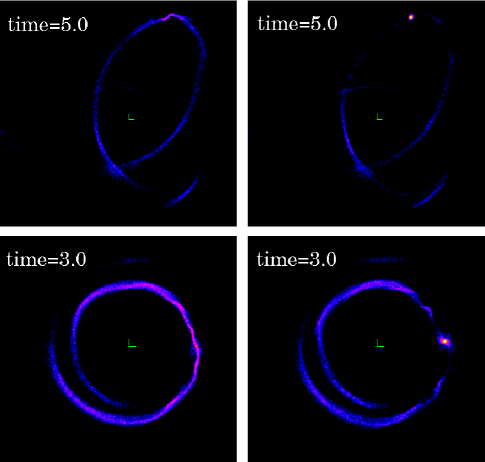
Figure 5: Snapshots of the last stages of the NFW satellites’ evolution on both orbits inside a Milky Way–sized halo projected onto the orbital plane. The satellites constructed using the approximate Gaussian scheme are displayed on the left, with the self-consistent satellites presented on the right. The color-coded logarithmic density maps are shown (the brighter the color, the higher the density), and the elapsed time since the start of the simulation (upper left-hand corners) is given in units of the radial orbital period. The two top panels show results for the eccentric 5:1 orbit with an apocenter radius equal to $r_{\rm apo}=7.5\ r_{\rm s,host}$, where $r_{\rm s,host}$ is the scale radius of the host halo, whereas the two bottom panels present results for the circular orbit with orbital radius $r_{\rm{circ}}=3.7\ r_{\rm s,host}$. After $5$ and $3$ orbital periods, respectively, there is no sign of a self-bound core on the left-hand panels, indicative of the fact that the Maxwellian satellites have been completely disrupted by the strong tidal field. On the other hand, the self-consistent satellites clearly survive complete disruption for the same timescales, retaining a self-bound core.

The two top panels of Figure 5 show results for the eccentric orbit. The satellites lose mass continuously on account of the strong tidal field, and the material that has been stripped off forms the familiar tidal tails that trace the orbital path. At each pericentric passage, the satellites experience the strongest tidal shocks which result in an increase of the mass-loss rate (Gnedin, Hernquist & Ostriker 1999; Taffoni et al. 2003). The top left-hand panel shows that after approximatelly $5$ orbits, the Gaussian satellite has been fully disrupted. On the other hand, the evolution of the self-consistent satellite was completely different. In this case, we note that the satellite was not fully dissolved after $5$ orbits, retaining a conspicuous self-bound core (top right-hand panel). Similarly, the two bottom panels of Figure 5 show the evolution of the satellites on the circular orbit. The bottom left-hand panel demonstrates that the satellite generated with the Maxwellian approximation is completely disrupted after only three orbits. The self-consistent satellite, on the other hand, retains a self-bound core that survives the tidal stripping (bottom right-hand panel).

Figure 6: Bound satellite mass as a function of the orbital period for the eccentric (thick lines) and circular (thin lines) orbits described in the text. The solid lines indicate satellite models generated using the local Maxwellian approximation, while the dot-dashed lines indicate models generated using the exact phase-space DF. The large dots correspond to the self-consistent, anisotropic satellite placed on the circular orbit. The satellites follow the NFW density profile. Satellites constructed under the assumption that the local velocity field is Maxwellian are totally disrupted in a few orbits, whereas the self-consistent satellites survive for much longer in the same tidal field. The anisotropic self-consistent satellite loses mass much more efficiently than its self-consistent isotropic counterpart on the same orbit and external tidal field. The latter demonstrates that the development of a global bias towards radial orbits in the Maxwellian satellites is one of the key factors in their accelerated disruption.

In Figure 6 we perform a more quantitative comparison of the satellites’ evolution, by identifying the mass that remains self-bound as a function of time. For that purpose we use the group finder SKID (Stadel 2001), which has been extensively used to identify gravitationally bound groups in $N$-body simulations. The figure shows results for the eccentric (thick lines) and circular (thin lines) orbits. In both cases, the Maxwellian and self-consistent satellites correspond to the solid and dot-dashed lines, respectively. The difference between the two initialization schemes is apparent in this plot and supports the view that the equilibrium model satellites slowly lose mass but do not completely disrupt within the timescales of our simulations.

We performed additional numerical experiments with circular orbits of different radii, as well as eccentric orbits with different eccentricities, and always found the same result: model satellites generated under the assumption that their local velocity field is Maxwellian survive in the tidal field for a much shorter timescale than their self-consistent counterparts. The former models are not “born” in equilibrium, the rapid expansion of their centers makes their density profiles become significantly shallower, and their velocity dispersion tensors become more radially biased (Fig. 1). We find no difference between the mass-loss rate of the Maxwellian satellites after allowing them to relax for $10$ dynamical times at the half-mass radius and that experienced by the same satellites when placed directly in the external tidal field.

In order to demonstrate the importance of a radially anisotropic velocity distribution in accelerating the disruption of a satellite, we have used the procedure of § 2 to construct a self-consistent anisotropic NFW satellite identical to the ones used above and with an anisotropy radius of $r_{\rm a}=(4/3)\,r_{\rm vir}$. The model was placed on the same circular orbit as before, and we followed the evolution of its bound mass for three orbital periods. The large dots in Figure 6 present results for this run, indicating that a self-consistent, radially anisotropic satellite experiences more efficient tidal stripping than its isotropic, self-consistent counterpart on the same external tidal field and orbit. Particles on more radial orbits spend, on average, more time at larger radii and are therefore more easily removed by the tidal field. On the other hand, models that remain isotropic and retain their steep central density cusp throughout their orbital evolution are much harder to destroy. A full study of these processes requires a large suite of numerical simulations covering a wide parameter space, which is clearly beyond the scope of the present paper.

We refrain from speculating too much about the implications our results have for the survival of substructure in CDM halos: our models ignore the response of the host halo to the satellite, which will affect the satellites’ susceptibility to disruption. We do note, however, that the differences we find in the survival times of satellites are of cosmological relevance. The period of the circular orbit is of the order of $\sim 3$ Gyr. This means that in one case the satellite gets disrupted in less than $8$ Gyr, while in the other case it survives at least for a time comparable to a Hubble time. In the case of the eccentric orbit, both satellites would survive for a time comparable to the cosmic age, but the more pronounced dissolution of the Maxwellian satellite can change dramatically the morphological evolution of the baryonic component sitting at its center (Mayer et al. 2001) and, as is also clear from the top panels of Figure 5, the prominence of the tidal streams produced (Helmi & White 1999; Johnston, Sigurdsson & Hernquist 1999; Mayer et al. 2002). In addition, while these orbits are more representative of those of satellites inside a primary halo close to $z=0$, satellites infalling into the main halo at much higher redshift will have considerably shorter orbital times (Mayer et al. 2001; Taffoni et al. 2003), and hence the difference between the two models will clearly be one of survival versus disruption even for highly eccentric orbits.

5 SUMMARY

In order to understand the physical processes that shape galaxies and DM halos, it is often more advantageous to study idealized $N$-body models of isolated galaxies than to try to extract insight from lower resolution, less controllable cosmological simulations. Unfortunately, constructing models of isolated galaxies with specified properties is not straightforward, but in § 2 we have described a procedure for generating equilibrium $N$-body realizations for a class of spherical galaxy models. Despite their simplicity, these models provide very good descriptions of the density profiles of both real and simulated galaxies and halos.

A commonly used alternative way of constructing ICs for galaxy models is by making the local Maxwellian approximation. This method has the attraction of being very general and relatively easy to implement. In recent years it has been used in investigations of the tidal stripping of satellites, the survival of substructure inside DM halos, and the effects of bars on halo profiles, among others. However, it suffers from a dangerous flaw. In § 3 we have presented a detailed analysis of the evolution of the density profiles and velocity structure of models produced using this approximation and have demonstrated that they are not in equilibrium. Models that are constructed with a central density cusp (e.g., NFW models) and an isotropic velocity dispersion tensor relax to a state with a much shallower inner density slope and develop a global bias towards radial orbits.

This spurious evolution can have spectacular consequences, as demonstrated in § 4, where we investigated the survival times of satellites orbiting inside a deeper, static host potential. Compared to self-consistent satellites, Maxwellian satellites experience accelerated mass loss, leading to their artificial dissolution in only a few orbits. This is something that has to be taken into account when the goal is to explore the evolution of substructure in CDM halos (Taffoni et al. 2003; Hayashi et al. 2003). Disruption times change significantly with respect to the cosmic age in the two initialization schemes. The fact that the self-consistent satellites are very hard to destroy supports the claim that abundant substructure is a key feature of CDM models (Moore et al. 1999b; Klypin et al. 1999). An extensive parameter survey of the influence of central density slopes, concentration parameters, and peak circular velocities on the survival and evolution of substructure halos within CDM models will be addressed in a forthcoming paper (S. Kazantzidis, L. Mayer, & B. Moore 2004, in preparation).

References

- Athanassoula (2002) Athanassoula, E. 2002, ApJ, 569, L83
- Binney and Tremaine (1987) Binney, J., & Tremaine, S. 1987, Galactic Dynamics (Princeton: Princeton Univ. Press)(BT87)
- Boily, Kroupa & Peñarrubia-Garrido (2001) Boily, C. M., Kroupa, P., & Peñarrubia-Garrido, J. 2001, NewA, 6, 27
- Colpi et al (1999) Colpi, M., Mayer, L., & Governato, F. 1999, ApJ, 525, 720
- Dehnen (1993) Dehnen, W. 1993, MNRAS, 265, 250
- Debattista and Sellwood (2000) Debattista, V. P., & Sellwood, J. A. 2000, ApJ, 543, 704
- Eddington (1916) Eddington, A. S. 1916, MNRAS, 76, 572
- Eke et al (2001) Eke, V. R., Navarro, J. F., & Steinmetz, M. 2001, ApJ, 554, 114
- Evans (1993) Evans, N. W. 1993, MNRAS, 260, 191
- Font et al (2001) Font, A. S., Navarro, J. F., Stadel, J., & Quinn, T. 2001, ApJ, 563, L1
- Ghigna et al (1998) Ghigna, S., Moore, B., Governato, F., Lake, G., Quinn, T., & Stadel, J. 1998, MNRAS, 300, 146
- Ghigna et al (2000) ———.2000, ApJ, 544, 616
- Gnedin et al (1999) Gnedin, O. Y., Hernquist, L., & Ostriker, J. P. 1999, ApJ, 514, 109
- Hayashi et al (2003) Hayashi, E., Navarro, J. F., Taylor, J. E., Stadel, J., & Quinn, T. 2003, ApJ, 584, 541
- Helmi and White (1999) Helmi, A., & White, S. D. M. 1999, MNRAS, 307, 495
- Hernquist (1990) Hernquist, L. 1990, ApJ, 356, 359
- Hernquist (1993) ———.1993, ApJS, 86, 389
- Jaffe (1983) Jaffe, W. 1983, MNRAS, 202, 995
- Jing and Suto (2000) Jing, Y. P., & Suto, Y. 2000, ApJ, 529, L69
- Johnston et al (1999) Johnston, K. V., Sigurdsson, S., & Hernquist, L. 1999, MNRAS, 302, 771
- King (1966) King, I. R. 1966, AJ, 71, 64
- Klypin et al (1999) Klypin, A., Kravtsov, A. V., Valenzuela, O., & Prada, F. 1999, ApJ, 522, 82
- Klypin et al (2001) Klypin, A., Kravtsov, A. V., Bullock, J. S. & Primack, J. R. 2001, ApJ, 554, 903
- Kravtsov et al (1998) Kravtsov, A. V., Klypin, A., Bullock, J. S., & Primack, J. R. 1998, ApJ, 502, 48
- Kuijken and Dubinski (1994) Kuijken, K., & Dubinski, J. 1994, MNRAS, 269, 13
- Lynden-Bell (1962) Lynden-Bell, D. 1962, MNRAS, 124, 1
- Mayer et al (2001) Mayer, L., Governato, F., Colpi, M., Moore, B., Quinn, T., Wadsley, J., Stadel, J., & Lake, G. 2001, ApJ, 559, 754
- Mayer et al (2002) Mayer, L., Moore, B., Quinn, T., Governato, F., & Stadel, J. 2002, MNRAS, 336, 119
- (29) Merritt, D. 1985a, AJ, 90, 1027
- (30) ———.1985b, MNRAS, 214, 25P
- Mihos et al (1997) Mihos, J. C., McGaugh, S., & de Blok, W. J. G. 1997, ApJ, 477, L79
- Moore et al (1996) Moore, B., Katz, N., & Lake, G. 1996, ApJ, 457, 455
- Moore et al (1999a) Moore, B., Quinn, T., Governato, F., Stadel, J., & Lake, G. 1999a, MNRAS, 310, 1147
- Moore et al (1999b) Moore, B., Ghigna, S., Governato, F., Lake, G., Quinn, T., Stadel, J., & Tozzi, P. 1999b, ApJ, 524, L19
- Navarro et al (1996) Navarro, J. F., Frenk, C. S., & White, S. D. M. 1996, ApJ, 462, 563 (NFW)
- Osipkov (1979) Osipkov, L. P. 1979, Soviet Astron. Lett., 5, 42
- Plummer (1911) Plummer, H. C. 1911, MNRAS, 71, 460
- Press et al (1996) Press, W. H., Teukolsky, S. A., Vetterling, W. T, & Flannery, B. P. 1996, Numerical Recipes in Fortran 90 (2d ed.; Cambridge: Cambridge Univ. Press)
- Quin and Goodman (1986) Quinn, P. J., & Goodman, J. 1986, ApJ, 309, 472
- Spingel and White (1999) Springel, V., & White, S. D. M. 1999, MNRAS, 307, 162
- Stadel (2001) Stadel, J. 2001, Ph.D. thesis, Univ. Washington
- Stoehr et al (2002) Stoehr, F., White, S. D. M., Tormen, G., & Springel, V. 2002, MNRAS, 335, L84
- Taffoni et al (2003) Taffoni, G., Mayer, L., Colpi, M., & Governato, F. 2003, MNRAS, 341, 434
- Taylor and Babul (2001) Taylor, J. E., & Babul, A. 2001, ApJ, 559, 716
- Tremaine et al (1994) Tremaine, S., Richstone, D. O., Byun, Y. I., Dressler, A., Faber, S. M., Grillmair, C., Kormendi, J., & Lauer T. R. 1994, AJ, 107, 634
- van den Bosch et al (1999) van den Bosch, F., Lewis, G., Lake, G., & Stadel, J. 1999, ApJ, 515, 50
- Valenzuela and Klypin (2003) Valenzuela, O., & Klypin, A. 2003, MNRAS, 345, 406
- Velázquez and White (1995) Velázquez, H., & White, S. D. M. 1995, MNRAS, 275, 23L
- Velázquez and White (1999) ———.1999, MNRAS, 304, 254
- Zhao (1996) Zhao, H. S. 1996, MNRAS, 278, 488