Tomographic 3D-Modeling of the Solar Corona with FASR

Abstract

The Frequency-Agile Solar Radiotelescope (FASR) litteraly opens up a new dimension in addition to the 3D Euclidian geometry: the frequency dimension. The 3D geometry is degenerated to 2D in all images from astronomical telescopes, but the additional frequency dimension allows us to retrieve the missing third dimension by means of physical modeling. We call this type of 3D reconstruction Frequency Tomography. In this study we simulate a realistic 3D model of an active region, composed of 500 coronal loops with the 3D geometry $[x(s),y(s),z(s)]$ constrained by magnetic field extrapolations and the physical parameters of the density $n_{e}(s)$ and temperature $T_{e}(s)$ given by hydrostatic solutions. We simulate a series of 20 radio images in a frequency range of $\nu=0.1-10$ GHz, anticipating the capabilities of FASR, and investigate what physical information can be retrieved from such a dataset. We discuss also forward-modeling of the chromospheric and Quiet Sun density and temperature structure, another primary goal of future FASR science.

1 INTRODUCTION

Three-dimensional (3D) modeling of solar phenomena has always been a challenge with the available two-dimensional (2D) images, but is an utmost necessity to test physical models in a quantitative way. Since solar imaging telescopes never have been launched on multiple spacecraft that separate to a significant parallax angle from the Earth, no true 3D imaging or solar tomography (Davila 1994; Gary, Davis, & Moore 1998; Liewer et al. 2001) has been performed so far. The Solar TErrestrial RElations Observatory (STEREO), now being assembled and planned for launch in November 2005, will be the first true stereoscopic facility, mapping the Sun with an increasing separation angle of $22^{\circ}$ per year. Alternative approaches of 3D reconstruction methods utilize the solar rotation to vary the aspect angle (Altschuler 1979; Berton & Sakurai 1985; Koutchmy & Molodensky 1992; Aschwanden & Bastian 1994a,b; Batchelor 1994; Hurlburt et al. 1994; Zidowitz 1999; Koutchmy, Merzlyakov, & Molodensky 2001), but this method generally requires static structures over several days. An advanced form of solar rotation stereoscopy is the so-called dynamic stereoscopy method (Aschwanden et al. 1999, 2000a), where the 3D geometry of dynamic plasma structures can be reconstructed as long as the guiding magnetic field is quasi-stationary. Of course, 3D modeling with 2D constraints can also be attempted if a-priori assumptions are made for the geometry, e.g. using the assumption of coplanar and semi-circular loops (Nitta, VanDriel-Gestelyi, & Harra-Murnion 1999).

A new branch of 3D modeling is the combination of 2D images $I(x,y)$ with the frequency dimension $\nu$, which we call frequency tomography. There have been only very few attempts to apply this method to solar data, mainly because multi-frequency imaging was not available or had insufficient spatial resolution. There are essentially only three published studies that employ the method of frequency tomography: Aschwanden et al. (1995); Bogod & Grebinskij (1997); Grebinskij et al. (2000.).

In the first study (Aschwanden et al. 1995), gyroresonance emission above a sunspot was observed at 7 frequencies in both polarizations in the frequency range of $\nu=10-14$ GHz with the Owens Valley Radio Observatory (OVRO) during 4 days. From stereoscopic correlations the height levels $h(\nu)$ of each frequency could be determined above the sunspot. Correcting for the jump in height when dominant gyroresonance emission switches from the second ($s=2$) to the third harmonic ($s=3$), the magnetic field $B(\nu)=357({\nu}_{GHz}/s)$ [G] could then be derived as a function of height, $B(h)$, and was found to fit a classical dipole field $B(h)=B_{0}(1+h/h_{D})^{-3}$. Moreover, from the measured brightness temperature spectrum $T_{B}(\nu)$, using the same stereoscopic height measurement $h(\nu)$, also the temperature profile $T(h)$ as a function of height above the sunspot could be determined. This study represents an application of frequency tomography, additionally supported with solar rotation stereoscopy, and thus is subject to the requirement of quasi-stationary structures.

In the second study (Bogod & Grebinskij 1997), brightness temperature spectra $T_{B}(\nu)$ were measured in 36 frequencies in the wavelength range of $\lambda=2-32$ cm ($\nu=0.94-15$ GHz) with RATAN-600, from quiet-Sun regions, active region plages, and from coronal holes. A differential deconvolution method of Laplace transform inversion was then used to infer the electron temperature $T(\tau)$ as a function of the opacity $\tau$. This method does not yield the temperature as a function of an absolute height $h$, but if an atmospheric model [$T(h),n_{e}(h)$] is available as a function of height, the temperature as a function of the free-free (bremsstrahlung) opacity $T(\tau)$ can be calculated and compared with the observations.

In the third study (Grebinskij et al. 2000), the brightness temperature in both polarizations is measured as a function of frequency, i.e. $T_{B}^{RCP}(\nu)$ and $T_{B}^{LCP}(\nu)$. Since the magnetic field has a slightly different refractive index in the two circular polarizations, the free-free (bremsstrahlung) opacity is consequently also slightly different, so that the magnetic field $B(\nu)$ can be inferred. Again, a physical model [$T(h),n_{e}(h),B(h)$] is needed to predict $B(\nu)$ and to compare it with the observed spectrum $T_{B}(\nu)$.

The content of this paper is as follows: In Section 2 we simulate an active region, with the 3D geometry constrained by an observed magnetogram and the physical parameters given by hydrostatic solutions, which are used to calculate FASR radio images in terms of brightness temperature maps $T_{B}(x,y,\nu)$, and test how the physical parameters of individual coronal loops can be retrieved with FASR tomography. In Section 3 we discuss a few examples of chromospheric and Quiet-Sun corona modeling to illustrate the power and limitations of FASR tomography. In the final Section 5 we summarize some primary goals of FASR science that can be pursued with frequency tomography.

2 ACTIVE REGION MODELING

2.1 Simulation of FASR Images

Figure 1: Potential field extrapolation of SoHO/MDI magnetogram data from 1999 May 8, 0-1 UT.

Our aim is to build a realistic 3D model of an active region, in form of 3D distributions of the electron density $n_{e}(x,y,z)$ and electron temperature $T_{e}(x,y,z)$, which can be used to simulate radio brightness temperature maps $T_{B}(x,y,\nu)$ at arbitrary frequencies $\nu$ that can be obtained with the planned Frequency-Agile Solar Radiotelescope (FASR).

We start from a magnetogram recorded with the Michelson Doppler Imager (MDI) instrument onboard the Solar and Heliospheric Observatory (SoHO) on 1999 May 8, 0-1 UT. We perform a potential field extrapolation with the magnetogram as lower boundary condition of the photospheric magnetic field, to obtain the 3D geometry of magnetic field lines. We apply a threshold for the minimum magnetic field at the footpoints, which limits the number of extrapolated field lines to $n=500$. The projection of these 3D field lines along the line-of-sight onto the solar disk is shown in Fig.1. We basically see two groups of field lines, (1) a compact double arcade with low-lying field lines in an active region in the north-east quadrant of the Sun, and (2) a set of large-scale field lines that spread out from the eastern active region to the west and close in the western hemisphere. From this set of field lines we have constrained the 3D geometry of 500 coronal loops, defined by a length coordinate $s(x,y,z)$.

Figure 2: Distributions of loop lengths $L$, loop maximum temperatures $T_{e,max}$, loop minimum densities $n_{min}$, and maximum densities $n_{max}$. The distributions with thick linestyle correspond to $\approx 400$ loops in the compact arcade, while the distributions with thin linestyle correspond to the group of $\approx 100$ large-scale loops.

In a next step we fill the 500 loops with coronal plasma with density $n_{e}(s)$ and temperature functions $T_{e}(s)$ that obey hydrostatic solutions. For accurate analytical approximations of hydrostatic solutions we used the code given in Aschwanden & Schrijver (2002). Each hydrostatic solution is defined by three independent parameters: the loop length $L$, the loop base heating rate $E_{H0}$, and the heating scale height $s_{H}$. The momentum and energy balance equation (between the heating rate and radiative and conductive loss rate, i.e. $E_{H}(s)+E_{rad}(s)+E_{cond}(s)=0$, yields a unique solution for each parameter set $(L,s_{H},E_{H0})$. For the set of short loops located in the compact double arcade, which have have lengths of $L\approx 4-100$ Mm, we choose a heating scale height of $s_{H}=10$ Mm and base heating rates that are randomly distributed in the logarithmic interval of $E_{H0}=10^{-4},...,10^{-2}$ erg cm^-3 s^-1. For the group of long loops with lengths of $L\approx 100-800$ Mm, we choose near-uniform heating ($s_{H}=800$ Mm) and volumetric heating rates randomly distributed in the logarithmic interval of $E_{H0}=0.5\times 10^{-7},...,0.5\times 10^{-5}$ erg cm^-3 s^-1. This choice of heating rates produces a distribution of loop maximum temperatures (at the loop tops) of $T_{e}\approx 1-3$ MK, electron densities of $n_{e}\approx 10^{8},...,10^{10}$ cm^-3 at the footpoints, and $n_{e}\approx 10^{6},...,10^{9}$ cm^-3 at the loop tops. We show the distribution of loop top temperatures, loop base densities, and loop top densities in Fig.2. These parameters are considered to be realistic in the sense that they reproduce typical loop densities and temperatures observed with SoHO and TRACE, as well as correspond to the measured heating scale heights of $s_{H}\approx 10-20$ Mm (Aschwanden, Nightingale, & Alexander 2000b), for the set of short loops.

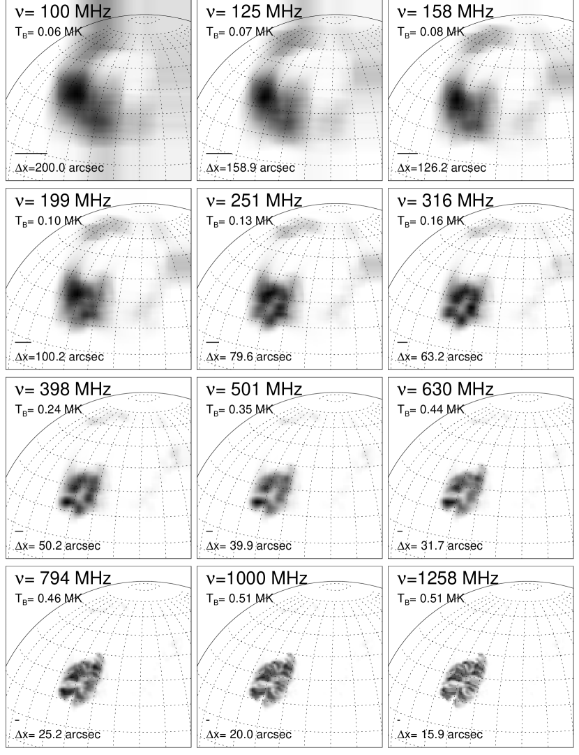
Figure 3: Simulation of radio brightness temperature maps of an active region at 20 frequencies, from $\nu$=100 to 1258 MHz. The maximum brightness temperature ($T_{B}$) and the angular resolution $\Delta x$ are indicated in each frame.

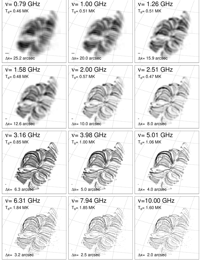
Figure 4: Similar representation as in Fig.3, for frequencies of $\nu$=0.8 to 10 GHz, with a smaller field-of-view than in Fig.3. The brightness is shown on linear scale in the first two rows, and on logarithmic scale in the last two rows (with a contrast of 1:100 in the third row and 1:1000 in forth row).

For the simulation of radio images we choose an image size of $512\times 512$ pixels, with a pixel size of 2.25”, and 21 frequencies logarithmically distributed between $\nu=100$ MHz and 10 GHz. To each magnetic field line we attribute a loop with a width (or column depth) of $w\approx 10^{8},...,10^{9}$ cm. For each voxel, i.e. volume element at ${\bf x}=(x_{i},y_{j},z_{k})$, we calculate the free-free absorption coefficient ${\kappa}_{ff}$ (e.g. Lang 1980, p.47),

$${\kappa}_{ff}^{\nu}(x_{i},y_{j},z_{k})=9.78\times 10^{-3}{n_{e,ijk}^{2}\over{\nu}^{2}T_{e,ijk}^{3/2}}[24.2+\ln{(T_{e,ijk})}-\ln{(\nu)}]\ ,$$ (1)

and integrate the opacity ${\tau}_{ff}^{\nu}$ along the line-of-sight $z$,

$${\tau}_{ff}^{\nu}(x_{i},y_{j},z_{k})=\int_{-\infty}^{z}{\kappa}_{ff}^{\nu}(x_{i},y_{j},z_{k})dz^{\prime}\ ,$$ (2)

to obtain the radio brightness temperature $T_{B}^{\nu}(x_{i},y_{j})$ with the radiative transfer equation (in the Rayleigh-Jeans limit),

$$T_{B}^{\nu}(x_{i},y_{j})=\int_{-\infty}^{+\infty}T_{e,ijk}\exp^{-{\tau}_{ff}^{\nu}((x_{i},y_{j},z_{k})}{\kappa}_{ff}^{\nu}(x_{i},y_{j},z_{k})dz\ ,$$ (3)

The simulated images for the frequency range of $\nu$=100 MHz to 10 GHz are shown in Figs.3 and 4. The approximate instrumental resolution is rendered by smoothing the simulated images with a boxcar that corresponds to the instrumental resolution of FASR,

$$w_{res}={20"\over{\nu}_{GHz}}.$$ (4)

A caveat needs to be made, that the real reconstructed radio images may reach this theoretical resolution only if a sufficient number of Fourier components are available, either from a large number of baselines (which scale with the square of the number of dishes) or from aperture synthesis (which increases the number of Fourier components during Earth rotation proportionally to the accumulation time interval). Also, we did not include here the effects of angular scattering due to turbulence or other coronal inhomogeneities (Bastian 1994, 1995).

2.2 Peak Brightness Temperature

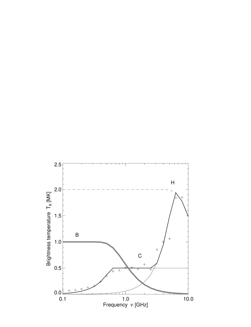
Figure 5: The radio peak brightness temperature $T_{B}$ is shown as function of frequency $\nu$: for the background corona (B), for cool (C) fat loops (T=0.5 MK, $n_{e}=10^{11}$ cm^-3, w=25 Mm), and hot (H) thin loops (T=2.0 MK, $n_{e}=10^{11}$ cm^-3, w=2.5 Mm). The cross symbols indicate the peak brightness temperatures observed in the simulated maps (Figs.3 and 4), while the medium-thick line represents the combined model of hot and cool loops. The dashed line indicates the expected brightness temperature of hot loops if no beam dilution due to the instrumental angular resolution would occur. The thick grey curve (B) indicates a model of the background corona.

The intensity of radio maps is usually specified in terms of the observed brightness temperature $T_{B}$. We list the peak brightness temperature in each map in Figs.3 and 4. We see that a maximum brightness is observed in the second-last map in Fig.4, with $T_{B}=1.85$ MK at a frequency of $\nu=7.94$ GHz. Let us obtain some understanding of the relative brightness temperatures $T_{B}(\nu)$ as function of frequency $\nu$, in order to faciliate the interpretation of radio maps. We plot the peak brightness temperature $T_{B}(\nu)$ of the simulated maps as function of frequency in Fig.5 (cross symbols). There are two counter-acting effects that reduce the brightness temperature: First, the loops become optically thin at high frequencies due to the ${\nu}^{-2}$-dependence of the free-free opacity (Eq.1). Hot loops with a temperature of T=2.0 MK, a density of $n_{e}=10^{11}$ cm^-3, and a width of w=2.5 Mm are optically thick below $\nu\lower 1.72218pt\hbox{$\;\buildrel<\over{\scriptstyle\sim}\;$}5$ GHz, so the brightness temperature would match the electron temperature $T_{B}=T_{e}$ (dashed line in Fig.5), but falls off at higher frequencies, i.e. $T_{B}(\nu>5$ GHz)$<T_{e}$.

The second effect that reduces the brightness temperature is the beam dilution, which has a ${\nu}^{2}$-dependence below the critical frequency where structures are unresolved. The effectively observed brightness temperature $T_{B}^{eff}(\nu)$ due to beam dilution for a structure with width $w$ is

$$T_{B}^{eff}(\nu)=T_{B}\times\left\{\begin{array}[]{cc}\left({\nu\over{\nu}_{crit}}\right)^{2}&{\rm for}\ \nu<{\nu}_{crit}(w)\\ 1&{\rm for}\ \nu>{\nu}_{crit}(w)\end{array}\right.$$ (5)

where the critical frequency ${\nu}_{crit}(w)$ depends on the width $w$ of the structure and is for FASR according to Eq.(4),

$${\nu}_{crit}(w)={20"\over w"}\ [GHz]\ .$$ (6)

Because the brightness drops drastically below ${\nu}_{crit}\approx 5$ GHz in Fig.5, we conclude that the width of the unresolved structures is about $w"=20"/5=4"=3$ Mm. Therefore we can understand the peak brightness temperatures in the maps, as shown in Fig.5 (crosses) in the range of $\nu\approx 3-10$ GHz with a combination of these two effects of free-free opacity and beam dilution.

Below a frequency of $\nu\lower 1.72218pt\hbox{$\;\buildrel<\over{\scriptstyle\sim}\;$}3$ GHz, we see that another group of loops contributes to the peak brightness of the maps. We find that the peak brightness below 3 GHz can adequately be understood by a group of cooler loops with a temperature of $T=0.5$ MK, densities of $n_{e}=10^{11}$ cm^-3, and widths of $w=25$ Mm (Fig.5). Thus cool loops dominate the brightness at low frequencies, and hot loops at higher frequencies.

In the simulations in Figs.3 and 4 we have not included the background corona. In order to give a comparison of the effect of the background corona we calculate the opacity for a space-filling corona with an average temperature of $T=1.0$ MK, an average density of $n_{e}=10^{9}$ cm^-3, and a vertical (isothermal) scale height of $w\approx{\lambda}_{T}\approx 50$ Mm. The brightness temperature of this background corona is shown with a thick grey curve (labeled B) in Fig.5. According to this estimate, the background corona overwhelms the brightest active region loops at frequencies of ${\nu}\lower 1.72218pt\hbox{$\;\buildrel<\over{\scriptstyle\sim}\;$}1$ GHz. From this we conclude that it might be difficult to observe active region loops at decimetric frequencies ${\nu}\lower 1.72218pt\hbox{$\;\buildrel<\over{\scriptstyle\sim}\;$}1.0$ GHz, unless they are very high and stick out above a density scale height, i.e. at altitudes of $h\lower 1.72218pt\hbox{$\;\buildrel>\over{\scriptstyle\sim}\;$}50$ Mm. In conclusion, the contrast of active region loops in our example seems to be best at frequencies of $\nu\approx 5$ GHz, but drops at both sides of this optimum frequency (see Fig.5).

Figure 6: The variation of the radio brightness temperature spectrum $T_{B}(\nu)$ of a loop by varying the temperature $T_{e}$ (top panel), the electron density $n_{e}$ (middle panel), and the loop width $w$ (bottom panel). In each of the three panels, one parameter is varied from 10%, 20%, …, 90% (dashed curves) to 110%, 120%,… , 200% (solid lines). The reference curve with parameters $T_{e}=1.0$ MK, $n_{e}=10^{10}$ cm^-3, and $w=10$ Mm is indicated with a thick line. The arrows indicate the spectral shift of the peak.

2.3 Temperature and Density Diagnostic of Loops

FASR will provide simultaneous sets of images $I(x,y,\nu)$ at many frequencies $\nu$. In other words, for every image position $(x_{i},y_{j})$, a spectrum $T_{B}^{ij}(\nu)$ can be obtained. A desirable capability is temperature and density diagnostic of active region loops. Let us parameterize the projected position of a loop by a length coordinate $s_{k}$, $k=1,...,n$, e.g. $[x_{i}=x(s_{k}),y_{j}=y(s_{k})]$. If we manage to determine the temperature $T_{e}(x_{i},y_{j})$ and density $n_{e}(x_{i},y_{i})$ at every loop position $(x_{i},y_{j})$, we have a diagnostic of the temperature profile $T(s)$ and density profile $n_{e}(s)$ of an active region loop. Thus, the question is whether we can manage to extract a temperature $T_{e}$ and density $n_{e}$ from a brightness temperature spectrum $T_{B}(\nu)$ at a given pixel position $(i,j)$. In order to illustrate the feasibility of this task, we show the brightness temperature spectrum $T_{B}(\nu)$ of a typical active region loop in Fig.6, and display its variation as a function of the physical ($T_{e}$, $n_{e}$) and geometric ($w$) parameters.

We define a typical active region loop by an electron temperature $T_{e}=1.0$ MK, an electron density $n_{e}=10^{10}$ cm^-3, and a width $w=10$ Mm. Such a loop is brightest at frequencies of $\nu\approx 1.5-3.0$ GHz (Fig.6; thick curve). The loop is fainter at higher frequencies because free-free emission becomes optically thin, while it is optically thick at lower frequencies. The reason why the loop is also fainter at low frequencies is because of the beam dilution at frequencies where the instrument does not resolve the loop diameter. If we increase the temperature, the brightness temperature increases, and vice versa decreases at lower electron temperatures (Fig.6 top). If we increase the density, the critical frequency where the loop becomes optically thin shifts to higher frequencies, while the peak brightness temperature decreases for lower densities (Fig.6, middle panel). If we increase the width of the loops, the brightness temperature spectrum is bright in a much larger frequency range, because we shift the critical frequency for beam dilution towards lower frequencies, while the overall brightness temperature decreases for a smaller loop width (Fig.6 bottom). Based on this little tutorial, one can essentially understand how the optimization works in spectral fitting (e.g. with a forward-fitting technique) to an observed brightness temperature spectrum $T_{B}(\nu)$.

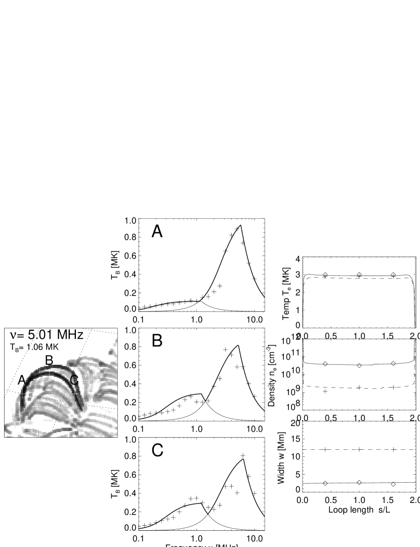
Figure 7: Enlarged detail of the active region with a bright loop (left panel). From the measured brightness temperature spectra $T_{B}(\nu)$ (crosses in middle panels) at the three loop locations (A,B,C) we fit theoretical spectra and determine the temperatures (right top panel), densities (right middle panel), and loop widths (right bottom panel) at the three loop locations (A,B,C).

To demonstrate how the density and temperature diagnostic works in practice, we pick a bright loop seen at ${\nu}=5.0$ GHz in Fig.4, which we show as an enlarged detail in Fig.7 (left panel). We pick three locations (A,B,C) along the loop and extract the brightness temperature spectra $T_{B}(\nu)$ from the simulated datacube $T_{B}(x,y,\nu)$ at the locations (A,B,C), shown in Fig.7 (three middle panels). Each spectrum shows two peaks, which we interpret as two cospatial loops. For each spectral peak we can therefore roughly fit a loop model, constrained by three parameters each, i.e. $[T_{e},n_{e},w]$. We can now fit a brightness temperature spectrum $T_{B}^{eff}(\nu)$ to the observed (or simulated here) spectrum $T_{B}^{obs}(\nu)$, physically defined by the same radiation transfer model for free-free emission as in Eqs.(1-5), but simplified by the approximation of constant parameters $(T_{e},n_{e})$, and thus a constant absorption coefficient ${\kappa}_{ff}(\nu)$, over the relatively small spatial extent of a loop diameter $w$,

$${\kappa}_{ff}(\nu)=9.78\times 10^{-3}{n_{e}^{2}\over{\nu}^{2}T_{e}^{3/2}}[24.2+\ln{(T_{e})}-\ln{(\nu)}]\ ,$$ (7)

$${\tau}_{ff}(\nu)={\kappa}_{ff}(\nu)\ w\ ,$$ (8)

$$T_{B}(\nu)=T_{e}\left(1-\exp^{-{\tau}_{ff}(\nu)}\right),$$ (9)

$$T_{B}^{eff}(\nu)=T_{B}\times\left\{\begin{array}[]{cc}\left({\nu\over{\nu}_{crit}}\right)^{2}&{\rm for}\ \nu<{\nu}_{crit}(w)\\ 1&{\rm for}\ \nu>{\nu}_{crit}(w)\end{array}\right.$$ (10)

What can immediately be determined from the observed brightness temperature spectra $T_{B}^{obs}(\nu)$ are the frequencies of the spectral peaks (Fig.7, middle panels), which are found around ${\nu}_{peak}=1.2$ and 6.0 GHz. Based on the tutorial given in Fig.6 it is clear that these spectral peaks demarcate the critical frequencies where structures become unresolved. Thus we can immediately determine the diameters of the two loops with Eq.(6), i.e. $w_{1}=20"/1.2=17"=12.0$ Mm and $w_{2}=20"/6.0=3.3"=2.4$ Mm. The only thing left to do is to vary the temperature and density and to fit the model (Eqs.7-10) to the observed spectrum. For an approximate solution (shown as smooth curves in the middle panels of Fig.7) we find $T_{1}=3.0$ MK and $n_{1}=4\times 10^{10}$ cm^-3 for the first loop (with width $w_{1}=2.5$ Mm and spectral peak at ${\nu}_{1}=6.0$ GHz), and $T_{2}=2.9$ MK and $n_{2}=1.9\times 10^{9}$ cm^-3 for the second loop (with width $w_{2}=12$ Mm and spectral peak at ${\nu}_{1}=1.2$ GHz). The resulting temperature $T_{e}(s)$ and density profiles $n_{e}(s)$ along the loops are shown in Fig.7 (right panels). This approximate fit is just an example to illustrate the concept of forward-fitting to FASR tomographic data. More information can be extracted from the data by detailed fits with variable loop cross-section along the loop and proper deconvolution of the projected column depth across the loop diameter (which is a function of the aspect angle between the line-of-sight and the loop axis). For a proper determination of the inclination angle of the loop plane, the principle of dynamic stereoscopy can be applied (Aschwanden et al. 1999; see Appendix A therein for coordinate transformations between the observers reference frame and the loop plane). Of course, our example is somehow idealized, in practice there will be confusion by adjacent or intersecting loops, as well as confusion by other radiation mechanisms, such as gyroresonance emission that competes with free-free emission at frequencies of $\nu\lower 1.72218pt\hbox{$\;\buildrel>\over{\scriptstyle\sim}\;$}5$ GHz near sunspots.

2.4 Radio versus EUV and soft X-ray diagnostics

We can ask whether temperature and density diagnostic of coronal loops is better done in other wavelengths, such as in EUV and soft X-rays (e.g. Aschwanden et al. 1999), rather than with radio tomography. Free-free emission in EUV and soft X-rays is optically thin, which has the advantage that every loop along a line-of-sight is visible to some extent, while loops in optically thick plasmas can be hidden at radio wavelengths. On the other side, the line-of-sight confusion in optically thin plasmas is larger in EUV and soft X-rays, in particular if multiple loops along the same line-of-sight have similar temperatures. Different loops along a line-of-sight can only be discriminated in EUV and soft X-rays if they have significantly different temperatures, so that they show different responses in lines with different ionization temperatures. Two cospatial loops that have similar temperatures but different widths cannot be distinguished by EUV or soft X-ray detectors. In radio wavelengths, however, even cospatial loops with similar temperatures, as the two loops in our example in Fig.7 ($T_{1}=3.0$ MK and $T_{2}=2.9$ MK), can be separated if they have different widths. The reason is that they have different critical frequencies ${\nu}_{crit}(w)$ where they become resolved, and thus show up as two different peaks in the brightness temperature spectrum $T_{B}^{eff}(\nu)$. Radio tomography has therefore a number of unique advantages over loop analysis in EUV and soft X-ray wavelengths: (1) a ground-based instrument is much less costly than a space-based instrument, (2) a wide spectral radio wavelength range (decimetric, centimetric) provides straightforwardly diagnostic over a wide temperature range, while an equivalent temperature diagnostic in EUV and soft X-rays would require a large number of spectral lines and instrumental filters, (3) optically thick radio emission is most sensitive to cool plasma, which is undetectable in EUV and soft X-rays, except for absorption in the case of very dense cool plasmas, and (4) radio brightness temperature spectra can discriminate multiple cospatial structures with identical temperatures based on their spatial scale, which is not possible with optically thin EUV and soft X-ray emission.

3 CHROMOSPHERIC AND CORONAL MODELING

The vertical density and temperature structure of the chromosphere, transition region, and corona has been probed in soft X-rays, EUV, and in radio wavelengths, but detailed models that are consistent in all wavelengths are still unavailable. Comprehensive coverage of the multi-thermal and inhomogeneous solar corona necessarily requires either many wavelength filters in soft X-rays and EUV, or many radio frequencies, for which FASR will be the optimum instrument.

We illustrate the concept of how to explore the vertical structure of the chromosphere and corona with a few simple examples. We know that the corona is highly inhomogeneous along any line-of-sight, so a 3D model has to be composed of a distribution of many magnetic fluxtubes, each one representing a mini-atmosphere with its own density and temperature structure, being isolated from each other due to the low value of the plasma-beta, i.e. $\beta=p_{thermal}/p_{magn}=2n_{e}k_{B}T_{e}/(B^{2}/8\pi)\ll 1$. The confusion due to inhomogeneous temperatures and densities is largest for line-of-sights above the limb (due to the longest column depths with contributing opacity), and is smallest for line-of-sights near the solar disk center, where we look down through the atmosphere in vertical direction.

The simplest model of the atmosphere is given by the hydrostatic equilibrium in the isothermal approximation, $T(h)=const$, where the hydrostatic scale height ${\lambda}_{T}$ is proportional to the electron temperature $T$, i.e.

$${\lambda}_{T}={k_{B}T\over\mu m_{p}g_{\odot}}={\lambda}_{0}\Bigl{(}{T\over 1\ {\rm MK}}\Bigr{)}\$$ (11)

with ${\lambda}_{0}=47$ Mm for coronal conditions, with $\mu m_{p}$ the average ion mass (i.e. $\mu\approx 1.3$ for H:He=10:1) and $g_{\odot}$ the solar gravitation. The height dependence of the electron density is for gravitational pressure balance,

$$n_{e}(h)=n_{0}\ \exp\bigl{[}-{(h-h_{0})\over{\lambda}_{0}T}\bigr{]}\ .$$ (12)

where $n_{0}=n(h_{0})$ is the base electron density. This expression for the density $n_{e}(h)$ can then be inserted into the free-free absorption coefficient ${\kappa}(h,\nu)$, with $T(h)=const$ in the isothermal approximation,

$${\kappa}_{ff}(h,\nu)=9.78\times 10^{-3}{n_{e}^{2}(h)\over{\nu}^{2}T(h)^{3/2}}[24.2+\ln{T(h)}-\ln{(\nu)}]\ ,$$ (13)

At disk center, we can set the altitude $h$ equal to the line-of-sight coordinate $z$, so that the free-free opacity ${\tau}_{ff}(h,\nu)$ integrated along the line-of-sight $h=z$ is,

$${\tau}_{ff}(h,\nu)=\int_{-\infty}^{h}{\kappa}_{ff}(h^{\prime},\nu)\ dh^{\prime}\ ,$$ (14)

and the radio brightness temperature $T_{B}(\nu)$ is then

$$T_{B}(\nu)=\int_{-\infty}^{0}T(h)\exp^{-{\tau}_{ff}(h,\nu)}{\kappa}_{ff}(h,\nu)dh\ .$$ (15)

With this simple model we can determine the mean temperature $T(h)$ by fitting the observed brightness temperature spectra $T_{B}(\nu)$ to the theoretical spectra (Eq.15) by varying the temperature $T(h)=const$ (in Eqs.13-14). The expected brightness temperature spectra for an isothermal corona with temperatures of $T=1.0$ MK and $T=5.0$ MK and a base density of $n_{0}=10^{9}$ cm^-3 are shown in Fig.8. We see that the corona becomes optically thin ($T_{B}\ll T_{e}$) at frequencies of ${\nu}\lower 1.72218pt\hbox{$\;\buildrel>\over{\scriptstyle\sim}\;$}1-2$ GHz in this temperature range that is typical for the Quiet Sun.

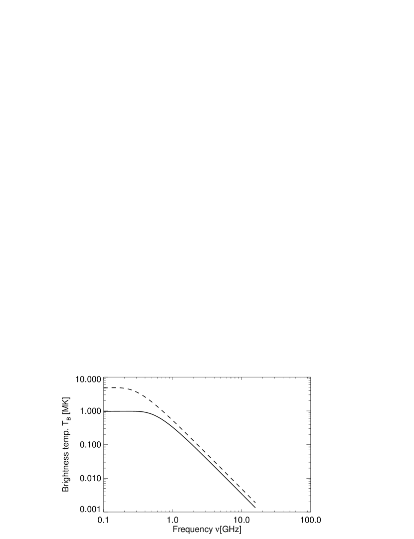
Figure 8: Quiet Sun brightness temperature spectrum for an isothermal corona with $T=1.0$ MK (solid line) or $T=5.0$ MK (dashed line) with a base density of $n_{0}=10^{9}$ cm^-3.

Figure 9: A compilation of chromospheric and coronal density models: VAL-C = Vernazza, Avrett, & Loeser (1981), model C; FAL-C = Fontenla, Avrett, & Loeser (1990), model C; FAL-P = Fontenla, Avrett, & Loeser (1990), model P; G = Gu, Jefferies et al. (1997); MM = Maltby et al., (1986), model M; ME = Maltby et al., (1986), model E; D = Ding & Fang (1989); O = Obridko & Staude (1988); Gabriel = Gabriel (1976), coronal model; CICM = Caltech Irreference Chromospheric Model, radio sub-millimeter limb observations (Ewell et al. 1993), RHESSI flare loop (Aschwanden, Brown, & Kontar 2002).

These hydrostatic models in the lower corona, however, have been criticized because of the presence of dynamic phenomena, such as spiculae, which may contribute to an extended chromosphere in the statistical average. The spicular extension of this dynamic chromosphere has been probed with high-resolution measurements of the Normal Incidence X-Ray Telescope (NIXT) (Daw, DeLuca, & Golub 1995) as well as with radio submillimeter observations during a total eclipse (Ewell et al. 1993). Using the radio limb height measurements at various mm and sub-mm wavelengths in the range of 200-3000 $\mu$m (Roellig et al. 1991; Horne et al. 1981; Wannier et al. 1983; Belkora et al. 1992; Ewell et al. 1993), an empirical Caltech Irreference Chromospheric Model (CICM) was established, which fits the observed limb heights between 500 km and 5000 km in a temperature regime of $T=4410$ K to $T=7500$ K (Ewell et al. 1993), shown in Fig.9. We see that these radio limb measurements yield electron densities that are 1-2 orders of magnitude higher in the height range of 500-5000 km than predicted by hydrostatic models (VAL, FAL, Gabriel 1976), which was interpreted in terms of the dynamic nature of spiculae (Ewell et al. 1993). This enhanced density in the extended chromosphere has also been corroborated with recent RHESSI measurements (Fig.8; Aschwanden, Brown, & Kontar 2002). Hard X-rays mainly probe the total neutral and ionized hydrogen density that governs the bremsstrahlung and the total bound and free electron density in collisional energy losses, while the electron density $n_{e}(h)$ inferred from the radio-based measurements is based on free-free emission, and shows a remarkably good agreement in the height range of $h\approx 1000-3000$ km. The extended chromosphere produces substantially more opacity at microwave frequencies than hydrostatic models (e.g. Gabriel 1976).

Figure 10: Quiet Sun brightness temperature spectrum for an isothermal corona with $T=1.5$ MK with a base density of $n_{0}=10^{9}$ cm^-3 (solid thin line), for the coronal model by Gabriel (1976) (thin solid line), and for a modified Gabriel model (thick solid line).

The atmospheric structure thus needs to be explored with more general parameterizations of the density $n_{e}(h)$ and temperature $T_{e}(h)$ structure than hydrostatic models provide. For instance, each of the atmospheric models shown in Fig.9 provides different functions $n_{e}(h)$ and $T_{e}(h)$. Observational tests of these models can simply be made by forward-fitting of the parameterized height-dependent density $n_{e}(h)$ and temperature profiles $T_{e}(h)$, using the expressions for free-free emission (Eqs.13-15). In Fig.10 we illustrate this with an example. The datapoints (shown as diamonds in Fig.10) represent radio observations of the solar limb at frequencies of ${\nu}=1.4-18$ GHz during the solar minimum in 1986-87 by Zirin, Baumert, & Hurford (1991). We show in Fig.10 an isothermal hydrostatic model for a coronal temperature of $T_{e}=1.5$ MK and a base density of $n_{e}=10^{9}$ cm^-3, as well as the hydrostatic model of Gabriel (1976), of which the density profile $n_{e}(h)$ is shown in Fig.9. The Gabriel model was calculated based on the expansion of the magnetic field of coronal flux tubes over the area of a supergranule (canopy geometry). The geometric expansion factor and the densities at the lower boundary in the transition region (given by the chromospheric VAL and FAL models, see Fig.9) then constrains the coronal density model $n_{e}(h)$, which falls off exponentially with height in an isothermal fluxtube in hydrostatic equilibrium. We see that the Gabriel model roughly matches the isothermal hydrostatic model (see Fig.10), but does not exactly match the observations by Zirin et al. (1991). However, if we multiply the Gabriel model by a factor of 0.4, to adjust for solar cycle minimum conditions, and add a temperature of $T_{e}=11,000$ K to account for an optically thick chromosphere (similar to the values determined by Bastian, Dulk, and Leblanc 1996), we find a reasonably good fit to the observations of Zirin (thick curve in Fig.10). This example demonstrates that radio spectra in the frequency range of ${\nu}\approx 1-10$ GHz are quite sensitive to probe the physical structure of the chromosphere and transition region.

4 FUTURE FASR SCIENCE

With our study we illustrated some basic applications of frequency tomography as can be expected from FASR data. We demonstrated how physical parameters from coronal loops in active regions, from the Quiet-Sun corona, and from the chromosphere and transition region can be retrieved. Based on these capabilities we expect that the following science goals can be efficiently studied with future FASR data:

1. The electron density $n_{e}(s)$ and electron temperature profile $T_{e}(s)$ of individual active region loops can be retrieved, which constrain the heating function $E_{H}(s)$ along the loop in the momentum and energy balance hydrodynamic equations. This enables us to test whether a loop is in hydrostatic equilibrium or evolves in a dynamic manner. Detailed dynamic studies of the time-dependent heating function $E_{H}(s,t)$ may reveal the time scales of intermittent plasma heating processes, which can be used to constrain whether AC or DC heating processes control energy dissipation. Ultimately, such quantitative studies will lead to the determination and identification of the so far unknown physical heating mechanisms, a long-thought goal of the so-called coronal heating problem. Radio diagnostic is most sensitive to cool dense plasma, but is also sensitive continuously up to the highest temperatures, and this way nicely complements EUV and soft X-ray diagnostic.

2. Because coronal loops are direct tracers of closed coronal magnetic field lines, the reconstruction of the 3D geometry of loops, as it can be mapped out with multi-frequency data from FASR in a tomographic manner, this information can be used to test theoretical models based on magnetic field extrapolations from the photosphere. The circular polarization of free-free emission contains additional information on the magnetic field (Grebinskij et al. 2000; Gelfreikh 2002; Brosius 2002), as well as gyroresonance emission provides direct measurements of the magnetic field by its proportionality to the gyrofrequency (Lee et al. 1998; White 2002; Ryabov 2002). Ultimately, such studies may constrain the non-potentiality and the localization of currents in the corona.

3. The density $n_{e}(h)$ and temperature profile $T_{e}(h)$ of the chromosphere, transition region, and corona can be determined in the Quiet Sun from brightness temperature spectra $T_{B}(\nu)$, with least confusion at disk center. Parameterized models of the density and temperature structure, additionally constrained by the hydrodynamic equations and differential emission measure distributions, can be forward-fitted to the observed radio brightness temperature spectra $T_{B}(\nu)$. This provides a new tool to probe physical conditions in the transition region, deviations from hydrostatic equilibria, and diagnostic of dynamic processes (flows, turbulence, waves, heating, cooling) in this little understood interface to the corona.

4. Since free-free emission is most sensitive to cool dense plasma, FASR data will also be very suitable to study the origin, evolution, destabilization, and eruption of filaments, which seem to play a crucial role in triggering and onset of coronal mass ejections (Vourlidas 2002). Ultimately, the information to forecast CMEs may be chiefly exploited from the early evolution of filaments.

Previous studies with multi-frequency instruments (VLA, OVRO, Nançay, RATAN-600) allowed only crude attempts to pioneer tomographic 3D-modeling of the solar corona, because of the limitations of a relatively small number of Fourier components and a sparse number of frequencies. FASR will be the optimum instrument to faciliate 3D diagnostic of the solar corona on a routine basis, which is likely to lead to groundbreaking discoveries in long-standing problems of coronal plasma physics.

References

- [1]
- [] Altschuler,M.D. 1979, in Image Reconstruction from Projections, (ed. G.T.Herman, Berlin:Springer, p.105
- [] Aschwanden,M.J. and Bastian,T.S. 1994a, Astrophys.J. 426, 425
- [] Aschwanden,M.J. and Bastian,T.S. 1994b, Astrophys.J. 426, 434
- [] Aschwanden,M.J., Lim,J., Gary,D.E., and Klimchuk,J.A. 1995, Astrophys.J. 454, 512
- [] Aschwanden,M.J., Newmark,J.S., Delaboudiniere,J.P., Neupert,W.M., Klimchuk,J.A., Gary,G.A., Portier-Fornazzi,F., and Zucker,A. 1999, Astrophys.J. 515, 842
- [] Aschwanden,M.J., Alexander,D., Hurlburt,N., Newmark,J.S., Neupert,W.M., Klimchuk,J.A., and G.A.Gary 2000a, Astrophys.J. 531, 1129
- [] Aschwanden,M.J., Nightingale,R.W., and Alexander,D. 2000b, Astrophys.J. 541, 1059
- [] Aschwanden,M.J. and Schrijver,K.J. 2002, Astrophys.J.Suppl.Ser. 142, 269
- [] Aschwanden,M.J., Brown,J.C., and Kontar,E.P. 2002, Solar Phys. (in press)
- [] Bastian,T.S. 1994, Astrophys.J. 426, 774
- [] Bastian,T.S. 1995, Astrophys.J. 439, 494
- [] Bastian,T.S., Dulk,G.A., and Leblanc,Y. 1996, Astrophys.J. 473, 539
- [] Batchelor,D.A. 1994, Solar Phys. 155, 57
- [] Belkora,L., Hurford,G.J., Gary,D.E. and Woody,D.P. 1992, Astrophys.J. 400, 692
- [] Berton.R. and Sakurai,T. 1985, Solar Phys. 96, 93
- [] Bogod,V.M., and Grebinskij,A.S. 1997, Solar Phys. 176, 67
- [] Brosius,J.W. 2002, (in this volume)
- [] Davila,J.M. 1994, Astrophys.J. 423, 871
- [] Daw,A., DeLuca,E.E., and Golub,L. 1995, Astrophys.J. 453, 929
- [] Ding, M.D. and Fang, C. 1989, Astron.Astrophys. 225, 204.
- [] Ewell, M.W.Jr., Zirin, H., Jensen, J.B., and Bastian, T.S. 1993, Astrophys.J. 403, 426.
- [] Fontenla, J.M., Avrett, E.H., and Loeser, R. 1990, Astrophys.J. 355, 700.
- [] Gabriel, A.H. 1976, Royal Society (London), Philosophical Transactions, Series A, 281, no. 1304, p. 339.
- [] Gary,A., Davis,J.M., and Moore,R. 1998, Solar Phys. 183, 45
- [] Gelfreikh,G.B. 2002, (in this volume)
- [] Grebinskij,A., Bogod,V., Gelfreikh,G., Urpo,S., Pohjolainen,S. and Shibasaki,K. 2000, Astron.Astrophys.Suppl.Ser. 144, 169
- [] Gu, Y., Jefferies, J.T., Lindsey, C. and Avrett, E.H. 1997, Astrophys.J. 484, 960.
- [] Horne, K., Hurford, G.J., Zirin, H., and DeGraauw, Th. 1981, Astrophys.J. 244, 340.
- [] Hurlburt,N.E., Martens,P,C.H., Slater,G.L., and Jaffey,S.M. 1994, in Solar Active Region Evolution: Comparing Models with Observations, ASP Conf. Ser. 68, 30
- [] Lang,K.R. 1980, Astrophysical Formulae. A Compendium for the Physicist and Astrophysicist, Berlin: Springer
- [] Lee,J.W., McClymont,A.N., Mikic,Z., White,S.M., and Kundu,M.R. 1998, Astrophys.J. 501, 853
- [] Koutchmy,S., and Molodensky,M.M. 1992, Nature 360, 717
- [] Koutchmy,S., Merzlyakov, V. L., and Molodensky, M. M. 2001, Astronomy Reports 45/10, 834
- [] Liewer,P.C., Hall,J.R., DeJong,M., Socker,D.G., Howard,R.A., Crane,P.C., Reiser,P., Rich,N., Vourlidas,A. 2001, J.Geophys.Res. 106/A8, 15903
- [] Maltby, P., Avrett, E.H., Carlsson, M., Kjeldseth-Moe, O., Kurucz, R.L., and Loeser, R. 1986, Astrophys.J. 306, 284.
- [] Nitta,N., VanDriel-Gestelyi,L., and Harra-Murnion,L,K. 1999, Solar Phys. 189, 181
- [] Obridko, V.N. and Staude, J. 1988, Astron.Astrophys. 189, 232.
- [] Roellig, T.L., Becklin, E.E., Jefferies, J.T., Kopp, G.A., Lindsey, C.A., Orral, F.Q., and Werner, M.W., 1991, Astrophys.J. 381, 288.
- [] Ryabov,V.B. 2002, (in this volume)
- [] Vernazza, J.E., Avrett, E.H., and Loeser, R. 1981, Astrophys.J.Suppl.Ser. 45, 635.
- [] Vourlidas,A. 2002, (in this volume)
- [] Wannier, P.G., Hurford, G.J., and Seielstad, G.A. 1983, Astrophys.J. 264, 660.
- [] White,S.M. 2002, (in this volume)
- [] Zidowitz,S. 1999, J.Geophys.Res. 104/A5, 9727
- [] Zirin,H., Baumert,B.M., and Hurford,G.J. 1991, Astrophys.J. 370, 779