Ideal MHD solution to the $\sigma$ problem in Crab-like pulsar winds
and General Asymptotic Analysis of Magnetized Outflows

Abstract

Using relativistic, steady, axisymmetric, ideal magnetohydrodynamics (MHD) we analyze the super-Alfvénic regime of a pulsar wind by means of solving the momentum equation along the flow as well as in the transfield direction. Employing a self-similar model, we demonstrate that ideal MHD can account for the full acceleration from high ($\gg 1$) to low ($\ll 1$) values of $\sigma$, the Poynting-to-matter energy flux ratio. The solutions also show a transition from a current-carrying to a return-current regime, partly satisfying the current-closure condition. We discuss the kind of the boundary conditions near the base of the ideal MHD regime that are necessary in order to have the required transition from high to low $\sigma$ in realistic distances, and argue that this is a likely case for an equatorial wind. Examining the MHD asymptotics in general, we extend the analysis of Heyvaerts & Norman and Chiueh, Li, & Begelman by including two new elements: classes of quasi-conical and parabolic field line shapes that do not preclude an efficient and much faster than logarithmic acceleration, and the transition $\sigma=\sigma_{c}$ after which the centrifugal forces (poloidal and azimuthal) are the dominant terms in the transfield force-balance equation.

1. Introduction

The spin down luminosity of a rotating pulsar powers the emission of an associated synchrotron nebula by driving an initially Poynting flux-dominated wind (the Poynting-to-matter energy flux ratio is $\sigma\gg 1$) that flows along the open magnetic field lines. The density of the outflowing matter is enhanced by pair-creating cascades near the source and the resulting number density is sufficiently large to screen the electric field along the flow and provide the necessary charge and current densities for ideal magnetohydrodynamics (MHD) to hold.

At a distance $r_{s}\approx 3\times 10^{17}$cm –specifically for the Crab – the ram pressure of the wind equals the total nebula pressure and the wind terminates in a standing shock (Rees & Gunn, 1974). The “wisps” (which appear at distance $\sim r_{s}$ from the center) are an observational signature of the coupling between the fast pulsar wind and the slowly expanding nebula (Hester et al., 1995). By applying ideal MHD in the nebula, the matching shock conditions require that the pulsar wind has become completely matter-dominated at the position of the shock; the $\sigma$ function should be as low as $\sigma_{s}=0.003$ just upstream of the termination shock (Kennel & Coroniti 1984a,b), and the question arises as to how this transition from high to low values of $\sigma$ can happen, the so-called $\sigma$ problem.

We note, however, that the very existence of the shock has been questioned by Blandford (2002), who argues that no shock is necessary and that the observed emission is created by current dissipation in a Poynting flux-dominated wind. Furthermore, even if a shock indeed terminates the pulsar wind, abandoning the axisymmetry or the ideal MHD in the nebula results in undetermined $\sigma_{s}$ (Begelman, 1998; Königl & Granot, 2002). Even so, $\sigma_{s}$ could in general be small, and the interpretation of the wisps as ion driven compressions (Arons, 2002), as well as the fitting of the observed nebula emission (Bogovalov & Khangoulian, 2002), provide additional support for the value $\sigma_{s}=0.003$.

The Crab-pulsar/nebula is the first and most analyzed object of this kind. Recent X-ray observations have shown that there exist other objects with common characteristics [e.g., the Vela pulsar (Helfand, Gotthelf, & Halpern, 2001), the nebulae associated with PSR B1509-58 (Gaensler et al., 2002), and PSR B1957+20 (Stappers et al., 2003)].

The study of approximately monopole magnetic field geometries that are extremely inefficient accelerators gave the impression to the community that ideal MHD is in general unable to solve the $\sigma$ problem, and many authors refer to the “$\sigma$ parameter” and not to the “$\sigma$ function”. Moreover, several alternative (non-ideal MHD) attempts (see, e.g., Arons, 1998 for a review) gave unsatisfactory results, and the puzzle remains unsolved for almost three decades. However, there are in the literature $r$ self-similar, ideal MHD solutions that start with $\sigma\gg 1$ near the origin of the flow and reach $\sigma_{\infty}\approx 1$ (Li, Chiueh, & Begelman, 1992; Vlahakis & Königl, 2003a), or even more efficient accelerators with $\sigma_{\infty}\approx 0.5$ (Vlahakis & Königl, 2003b), or $\sigma_{\infty}\approx 0.1$ (Vlahakis, Peng, & Königl, 2003). (Actually, $r$ self-similar are the only for the present known exact solutions of relativistic MHD in the sense that they satisfy the momentum equation in both directions: along the flow and in the transfield direction.) We note in this connection that the main acceleration mechanism is not the centrifugal, but the magnetic. The former may be important in the sub-Alfvénic regime of a disk-wind and results in poloidal velocity of the order of the initial Keplerian speed, while the latter – caused by the magnetic pressure-gradient force – results in much higher velocity that depends on the initial Poynting-to-mass flux ratio $\mu c^{2}$. Employing the $\sigma$ function we may write $\gamma_{\infty}=\mu/(1+\sigma_{\infty})$, thus the maximum final Lorentz factor is attained in solutions with $\sigma_{\infty}=0$. In this paper we show that ideal MHD can account for the full acceleration from $\sigma\gg 1$ to $\sigma\approx 0$, if the boundary condition $|I|>>A\Omega$ at the base of the ideal MHD accelerating regime is satisfied (here $I$ is the poloidal current, $A$ the poloidal magnetic flux function, and $\Omega$ the field angular velocity).

The transfield force-balance equation is the most important in determining the acceleration by means of controlling the field line shape and consequently how fast the quantity $\varpi^{2}B_{p}$ decreases (here $\varpi$ is the cylindrical distance and $B_{p}$ the poloidal magnetic field). In the main part of the acceleration the transfield component of the electromagnetic force equals the poloidal centrifugal force that is proportional to the curvature of the poloidal field lines $1/{\cal R}$. If this is still the case after the end of the acceleration – in the far-asymptotic regime where $\varpi/{\cal R}=0$ – the electromagnetic force exactly vanishes yielding the solvability condition at infinity (Heyvaerts & Norman, 1989; Chiueh, Li, & Begelman, 1991). However, if during the acceleration phase sufficiently small $\sigma$ values are reached, the azimuthal centrifugal force – the other part of the inertial force – becomes important. In this regime it is the difference between poloidal and azimuthal centrifugal forces that equals the much smaller electromagnetic force in the transfield direction, and no solvability condition can be derived.

We organize the paper as follows. In §2 we present the ideal MHD formalism focusing on the super-Alfvénic asymptotic regime where the puzzling transition from $\sigma\gg 1$ to $\sigma\ll 1$ happens. In §3 we derive a novel $z$ self-similar class of solutions describing the polar region of the wind and present the results of the integration. In §4 we analyze the asymptotic shape of the flow in relation to the acceleration, demonstrating that the same results are expected in non-self-similar cases as well. In §5 we discuss the problem of the pulsar magnetosphere, pointing out the problems that the force-free picture faces, and suggesting qualitatively a scenario that seems plausible for creating an equatorial wind with the appropriate conditions for efficient acceleration from high to low-$\sigma$ values satisfied. A summary follows in §6.

2. The steady - axisymmetric MHD description

2.1. Governing equations

The system of equations of special relativistic, steady, ideal MHD, consists of the Maxwell equations, Ohm’s law, and the continuity, entropy and momentum equations:

$${\boldsymbol{\nabla}}\cdot{\boldsymbol{B}}=0\,,\quad{\boldsymbol{\nabla}}\times{\boldsymbol{E}}=0\,,$$ (1a)

$${\boldsymbol{\nabla}}\times{\boldsymbol{B}}=4\pi{\boldsymbol{J}}/c\,,\quad{\boldsymbol{\nabla}}\cdot{\boldsymbol{E}}=4\pi J^{0}/c\,,\quad{\boldsymbol{E}}={\boldsymbol{B}}\times{\boldsymbol{V}}/c\,,$$ (1b)

$${\boldsymbol{\nabla}}\cdot\left(\rho_{0}\gamma{\boldsymbol{V}}\right)=0\,,\quad{\boldsymbol{V}}\cdot{\boldsymbol{\nabla}}\left({P}/{\rho_{0}^{\Gamma}}\right)=0\,,$$ (1c)

$$-\gamma\rho_{0}\left({\boldsymbol{V}}\cdot{\boldsymbol{\nabla}}\right)\left(\xi\gamma{\boldsymbol{V}}\right)-{\boldsymbol{\nabla}}P+\left(J^{0}{\boldsymbol{E}}+{\boldsymbol{J}}\times{\boldsymbol{B}}\right)/c=0\,.$$ (1d)

Here $\boldsymbol{V}$ is the velocity of the outflow, $\gamma$ the associated Lorentz factor, ${\boldsymbol{E}}\,,{\boldsymbol{B}}$ the electric and magnetic fields as measured in the central object’s frame, $J^{0}/c\,,{\boldsymbol{J}}$ the charge and current densities, $\rho_{0}\,,P$ the gas rest-mass density and pressure in the comoving frame, while for the polytropic equation of state (with index $\Gamma$) the enthalpy-to-rest-mass ratio is

$$\xi c^{2}=c^{2}+\frac{\Gamma}{\Gamma-1}\frac{P}{\rho_{0}}\,.$$ (2)

Assuming axisymmetry [$\partial/\partial\phi=0$, in spherical $\left(r\,,\theta\,,\phi\right)$ and cylindrical $\left(z\,,\varpi\,,\phi\right)$ coordinates with $\hat{z}$ along the rotation axis and the central object at ($\varpi=0\,,z=z_{c})$], five conserved quantities along the flow exist. If $A$ is the poloidal magnetic flux function, they are (e.g., Vlahakis & Königl 2003a):

$$\mbox{the mass-to-magnetic flux ratio}\ \Psi_{A}(A)=\frac{4\pi\gamma\rho_{0}V_{p}}{B_{p}}\,,$$ (3a)

$$\mbox{the field angular velocity}\ \Omega(A)=\frac{V_{\phi}}{\varpi}-\frac{V_{p}}{\varpi}\frac{B_{\phi}}{B_{p}}\,,$$ (3b)

$$\mbox{the specific angular momentum}\ L(A)=\xi\gamma\varpi V_{\phi}-\frac{\varpi B_{\phi}}{\Psi_{A}}\,,$$ (3c)

$$\mbox{the energy-to-mass flux ratio}\ \mu(A)c^{2}=\xi\gamma c^{2}-\frac{\varpi\Omega B_{\phi}}{\Psi_{A}}\,,$$ (3d)

$$\mbox{the adiabat}\ Q(A)=\frac{P}{\rho_{0}^{\Gamma}}\,,$$ (3e)

where subscripts $p$/$\phi$ denote poloidal/azimuthal components.

An important combination of the above field line constants is the “Michel’s magnetization parameter”

$$\sigma_{\rm M}(A)\equiv\frac{A\Omega^{2}}{\Psi_{A}c^{3}}\,.$$ (4)

The physical quantities can be expressed as functions of $A$ and the “Alfvénic” Mach number $M\equiv(\gamma V_{p}/B_{p})(4\pi\rho_{0}\xi)^{1/2}$:

$$\rho_{0}=\frac{\xi\Psi_{A}^{2}}{4\pi M^{2}}\,,$$ (5a)

$$\gamma=\frac{\mu}{\xi}\frac{M^{2}-(1-x_{\rm A}^{2})}{M^{2}+x^{2}-1}\,,$$ (5b)

$${\boldsymbol{B}}=\frac{{\boldsymbol{\nabla}}A\times\hat{\phi}}{\varpi}-\frac{c\Psi_{A}}{x}\left(\mu-\xi\gamma\right)\hat{\phi}\,,\quad{\boldsymbol{E}}=-\frac{\Omega}{c}{\boldsymbol{\nabla}}A\,,$$ (5c)

$$\frac{V_{p}}{c}=\frac{M^{2}B_{p}}{\xi\gamma\Psi_{A}c}\,,\quad\frac{V_{\phi}}{c}=\frac{\xi\gamma-\mu\left(1-x_{\rm A}^{2}\right)}{\xi\gamma x}$$ (5d)

Here $x=\varpi\Omega/c$ is the cylindrical distance in units of the light cylinder’s lever arm on each field-streamline $A=$const, and $x_{\rm A}=\left({L\Omega}/{\mu c^{2}}\right)^{1/2}$ is its value at the Alfvén point.

Alternatively, using the equivalent to equation (5b),

$$M^{2}=\frac{\xi\gamma}{\mu-\xi\gamma}x^{2}-\frac{\xi\gamma-\mu\left(1-x_{\rm A}^{2}\right)}{\mu-\xi\gamma}$$ (6)

and the Poynting-to-matter energy flux ratio

$$\sigma\equiv-\frac{\varpi\Omega B_{\phi}}{\Psi_{A}\xi\gamma c^{2}}=\frac{\mu-\xi\gamma}{\xi\gamma}\ \Leftrightarrow\ \xi\gamma=\frac{\mu}{1+\sigma}\,,$$ (7)

we may rewrite all quantities as functions of ($A\,,\gamma$) or ($A\,,\sigma$).

The two remaining equations are the Bernoulli and the transfield force-balance relations. The identity $\gamma^{2}-1=\left(\gamma V_{p}/c\right)^{2}+\left(\gamma V_{\phi}/c\right)^{2}$ gives the Bernoulli equation

$$\gamma^{2}-1=$$

$$=\Sigma^{2}\left[\frac{\mu\gamma}{\mu-\xi\gamma}-\mu\frac{\xi\gamma-\mu\left(1-x_{\rm A}^{2}\right)}{\xi\left(\mu-\xi\gamma\right)x^{2}}\right]^{2}+\left[\frac{\xi\gamma-\mu\left(1-x_{\rm A}^{2}\right)}{\xi x}\right]^{2}$$ (8)

where

$$\Sigma\equiv\frac{\Omega^{2}\varpi|{\boldsymbol{\nabla}}A|}{\mu\Psi_{A}c^{3}}\quad\left(=\frac{\sigma_{\rm M}}{\mu}\frac{\varpi^{2}B_{p}}{A}\right)\,.$$ (9)

The projection of equation (1d) along $\hat{n}\equiv-{\boldsymbol{\nabla}}A/|{\boldsymbol{\nabla}}A|$ gives the transfield force-balance equation

$${f}_{C\bot}+{f}_{I\bot}+{f}_{P\bot}+{f}_{EM1}+{f}_{EM2}+{f}_{EM3}=0\,,$$

where:

• The azimuthal centrifugal term

  $${f}_{C\bot}=\xi\gamma^{2}\rho_{0}\frac{V_{\phi}^{2}}{\varpi}\hat{n}\cdot\hat{\varpi}=\frac{B_{p}^{2}}{4\pi\varpi}\left(\frac{MV_{\phi}}{V_{p}}\right)^{2}\hat{n}\cdot\hat{\varpi}\,.$$

• The rest of the inertial force density along $\hat{n}$

  $${f}_{I\bot}=-\gamma^{2}\rho_{0}\xi\hat{n}\cdot\left[\left({\boldsymbol{V}}\cdot{\boldsymbol{\nabla}}\right){\boldsymbol{V}}\right]-{f}_{C\bot}=-\frac{B_{p}^{2}}{4\pi{\cal R}}M^{2}$$

  is the poloidal centrifugal term. Here ${\cal R}$ is the curvature radius of the poloidal field lines.

• The pressure gradient force density along $\hat{n}$

  $${f}_{P\bot}=-\hat{n}\cdot{\boldsymbol{\nabla}}P\,.$$

• The “electric field” force density

  $${f}_{E\bot}=\frac{1}{8\pi\varpi^{2}}\hat{n}\cdot{\boldsymbol{\nabla}}\left(\varpi^{2}E^{2}\right)-\frac{{E^{2}}}{{4\pi{\cal R}}}\,.$$

• The “magnetic field” force density along $\hat{n}$

  $${f}_{B\bot}=-\frac{1}{8\pi\varpi^{2}}\hat{n}\cdot{\boldsymbol{\nabla}}\left(\varpi^{2}B^{2}\right)+\frac{{B_{p}^{2}}}{{4\pi{\cal R}}}+\frac{B_{p}^{2}}{4\pi\varpi}\hat{n}\cdot\hat{\varpi}\,.$$

The total electromagnetic force density in the transfield direction $({f}_{E\bot}+{f}_{B\bot})$ can be decomposed as

$$\underbrace{-\frac{1}{8\pi\varpi^{2}}\hat{n}\cdot{\boldsymbol{\nabla}}\left[\varpi^{2}\left(B^{2}-E^{2}\right)\right]}_{f_{EM1}}+\underbrace{\frac{{B_{p}^{2}(1-x^{2})}}{{4\pi{\cal R}}}}_{f_{EM2}}+\underbrace{\frac{B_{p}^{2}}{4\pi\varpi}\hat{n}\cdot\hat{\varpi}}_{f_{EM3}}$$ (10)

Altogether, they give the following form of the transfield force-balance equation:

$$\frac{B_{p}^{2}}{4\pi{\cal R}}\left(M^{2}+x^{2}-1\right)=-\frac{1}{8\pi\varpi^{2}}\hat{n}\cdot{\boldsymbol{\nabla}}\left[\varpi^{2}\left(B^{2}-E^{2}\right)\right]+$$

$$+\frac{B_{p}^{2}}{4\pi\varpi}\left[1+\left(\frac{MV_{\phi}}{V_{p}}\right)^{2}\right]\hat{n}\cdot\hat{\varpi}-\hat{n}\cdot{\boldsymbol{\nabla}}P\,.$$ (11)

(Using equations [2.1], the latter becomes a second-order partial differential equation (PDE) for $A$.)

At the origin of the flow (subscript $i$), $x_{i}\ll x_{\rm A}$, $M_{i}^{2}\ll 1-x_{\rm A}^{2}$, and (using eq. [5b]) $\gamma_{i}\xi_{i}(1-x_{i}^{2})\approx\mu(1-x_{\rm A}^{2})$. As the flow moves downstream, the functions $x$ and $M$ increase, and when the Alfvén surface is reached they become $x=x_{\rm A}$, $M^{2}=1-x_{\rm A}^{2}$. The pulsar wind is still strongly magnetized in the neighborhood of the Alfvén surface, and the field is close to force-free there: $|{f}_{I\bot}|\ll|{f}_{B_{p}\bot}|$, or, $M^{2}\ll 1$, implying $x_{\rm A}\lesssim 1$. The light cylinder $x=1$ is located slightly after the Alfvén surface. Next, the flow enters the super-Alfvénic regime.

2.2. The super-Alfvénic asymptotic regime

In this regime $x^{2}\gg x_{\rm A}^{2}\approx 1$, $M^{2}\gg 1-x_{\rm A}^{2}$. Also thermal effects play no longer any role and the fluid is cold, $\xi\approx 1$. It is reasonable to assume that the above inequalities hold from the classical fast-magnetosound point downstream. At this point $(\gamma V_{p})^{2}\approx(B^{2}-E^{2})/4\pi\rho_{0}$, and for cold flows, $\gamma\approx\mu^{1/3}\gg 1$ (e.g., Camenzind 1986).
Employing the comoving magnetic field $B^{2}-E^{2}=B_{p}^{2}(1-x^{2})+B_{\phi}^{2}$, the Bernoulli equation (2.1) gives the exact result

$$B^{2}-E^{2}=\frac{x^{2}\left[x^{2}-1+\mu^{2}(1-x_{\rm A}^{2})^{2}/\xi^{2}\right]}{\left[x^{2}-1+\mu(1-x_{\rm A}^{2})/\xi\gamma\right]^{2}}\frac{B_{\phi}^{2}}{\gamma^{2}}\,.$$ (12)

In the asymptotic regime where $x\gg 1$ the latter equation implies

$$B^{2}-E^{2}\approx\frac{B_{\phi}^{2}}{\gamma^{2}}\,,\ \frac{x^{2}B_{p}^{2}}{B_{\phi}^{2}}=\frac{B_{\phi}^{2}-\left(B^{2}-E^{2}\right)}{B_{\phi}^{2}\left(1-1/x^{2}\right)}\approx\frac{1-1/\gamma^{2}}{1-1/x^{2}}\,.$$ (13)

Thus, the magnetic field is mainly azimuthal and the electric field approximately equals the magnetic field

$$E=\frac{\Omega}{c}|{\boldsymbol{\nabla}}A|=xB_{p}\approx-B_{\phi}\left(\frac{1-1/\gamma^{2}}{1-1/x^{2}}\right)^{1/2}\,.$$ (14)

The approximate form of the Bernoulli equation (2.1) is

$$\left({\gamma^{2}-1}\right)^{1/2}\approx\Sigma\frac{\mu\gamma}{\mu-\gamma}\,.$$ (15)

We are now in a position to examine the highly nonlinear transfield force-balance equation (2.1).

In that equation, the ${f}_{B\bot}$ and ${f}_{E\bot}$ are the dominant terms that almost cancel each other (e.g. Bogovalov 2001; Vlahakis & Königl 2003a). The algebraic sum of their main contributions is the $f_{EM1}$ term, which can be written as (using eq. [13]) $-(1/8\pi\varpi^{2})\hat{n}\cdot{\boldsymbol{\nabla}}\left(\varpi B_{\phi}/\gamma\right)^{2}$. This term must be balanced by the other terms of equation (2.1). Ignoring ${f}_{P\bot}$, we are left with the “poloidal curvature” term $(B_{p}^{2}/4\pi{\cal R})(M^{2}+x^{2}-1)=-f_{I\bot}-f_{EM2}$ and the term $-({B_{p}^{2}}/{4\pi\varpi})[1+({MV_{\phi}}/{V_{p}})^{2}]\hat{n}\cdot\hat{\varpi}=-f_{C\bot}-f_{EM3}$. Note that the last term, which henceforth we call “centrifugal”, has contributions from the poloidal magnetic field (the part $-f_{EM3}$ which is the dominant one in the $\sigma\gg 1$ regime), and from the azimuthal centrifugal force $-f_{C\bot}$. (The ratio of the two “centrifugal” parts is $f_{EM3}/f_{C\bot}\approx M^{2}/x^{2}\approx\sigma$, and the term $f_{C\bot}$ becomes important in the matter-dominated regime.) Thus, the asymptotic form of the transfield force-balance equation (2.1) is

$$(M^{2}+x^{2})\frac{\varpi}{{\cal R}}\approx-\frac{\hat{n}\cdot{\boldsymbol{\nabla}}}{2\varpi B_{p}^{2}}\left[\frac{\varpi B_{\phi}}{\gamma}\right]^{2}+\left[1+\frac{M^{2}\gamma^{2}}{x^{2}(\gamma^{2}-1)}\right]\hat{n}\cdot\hat{\varpi}\,.$$ (16)

This important equation, with the “centrifugal” term omitted, was derived by Chiueh et al. (1991); Lyubarsky & Eichler (2001); Okamoto (2002), while recently Tomimatsu & Takahashi (2003) derived the same equation with the “centrifugal” term included, but the poloidal curvature term omitted.

It is convenient to rewrite the Bernoulli and transfield force-balance equations in terms of the unknown functions ($A\,,\sigma$) (also assuming ${\gamma^{2}-1}\approx\gamma^{2}$). The Bernoulli equation (15) becomes $\gamma=\mu\left(1-\Sigma\right)$, or (using eqs. [7], and [9]),

$$\frac{\sigma}{1+\sigma}=\frac{\sigma_{\rm M}}{\mu}\frac{\varpi|{\boldsymbol{\nabla}}A|}{A}\quad\left(=\frac{\sigma_{\rm M}}{\mu}\frac{\varpi^{2}B_{p}}{A}\right)\,.$$ (17a)

The transfield force-balance equation (16) becomes (using eqs. [5c], [6], [7], and [17a])

$$\frac{\varpi}{{\cal R}}=\frac{\sigma(1+\sigma)\varpi{\boldsymbol{\nabla}}A\cdot{\boldsymbol{\nabla}}}{\mu^{2}|{\boldsymbol{\nabla}}A|}\ln\frac{A\Omega\sigma}{\sigma_{\rm M}}-\frac{c^{2}}{\varpi^{2}\Omega^{2}}\frac{\hat{\varpi}\cdot{\boldsymbol{\nabla}}A}{|{\boldsymbol{\nabla}}A|}\,.$$ (17b)

Equations (17a), and (17b) together with the equation for the curvature radius,

$${\cal R}=\frac{|{\boldsymbol{\nabla}}A|}{{\boldsymbol{\nabla}}^{2}A-{\boldsymbol{\nabla}}A\cdot{\boldsymbol{\nabla}}\ln|\varpi{\boldsymbol{\nabla}}A|}\,,$$ (17c)

form a closed system for the functions $\sigma$ and $A$. A possible solution of the system will describe the outflow downstream from the classical fast-magnetosound surface (where the super-Alfvénic asymptotic conditions surely hold).

Our task is to find a field geometry $A(\varpi\,,z)$, such that the flow accelerates smoothly from $\sigma\gg 1$ (at the classical fast-magnetosound surface) to $\sigma\ll 1$ (in the matter-dominated regime). Equation (17a) shows that the key quantity $\varpi|{\boldsymbol{\nabla}}A|=\varpi^{2}B_{p}$ should be a decreasing function of the distance from the source, along any field line. According to the model of Kennel & Coroniti (1984a,b) for the Crab nebula, the solution should give $\sigma_{s}\approx 0.003$, $\gamma_{s}\approx\mu\approx 10^{6}$, and $B_{\phi,{s}}\approx-2\times 10^{-5}$G, at the distance $r_{s}\approx 3\times 10^{17}$ cm of the termination shock. At the classical fast-magnetosound surface $\gamma_{f}\approx\mu^{1/3}=10^{2}$ and, from equation (7), $\sigma_{f}\approx 10^{4}$.

2.2.1 General solution characteristics

The current distribution
The number density of the particles in the pulsar magnetosphere highly exceeds the Goldreich-Julian value, and a tiny deviation from neutrality is enough to support the electromagnetic field. Assuming that in the upper (lower) hemisphere $B_{\phi}<0(>0)$, the Poynting-flux is outflowing when the electric field points toward the rotation axis, corresponding to a negative value of the charge density in the polar regions ($J^{0}<0$). For a highly relativistic poloidal motion,

$$J^{0}=\frac{c}{4\pi}{\boldsymbol{\nabla}}\cdot{\boldsymbol{E}}=-\frac{1}{4\pi}{\boldsymbol{\nabla}}\left({\boldsymbol{V}}\times{\boldsymbol{B}}\right)\approx\frac{1}{4\pi}{\boldsymbol{V}}_{p}\cdot{\boldsymbol{\nabla}}\times{\boldsymbol{B}}\approx J_{\parallel}$$

(where a suffix “$\parallel$” denotes the component of a vector along the poloidal field), and the flow that originates from the negatively-charged polar region is current-carrying ($J_{\parallel}<0$). The current-closure condition demands that each field line reaches a point where $J_{\parallel}=0$, and after that enters the distributed “return-current” regime $J_{\parallel}>0$. The poloidal current density is ${\boldsymbol{J}}_{p}=\frac{c}{4\pi}{\boldsymbol{\nabla}}\times{\boldsymbol{B}}_{\phi}=\frac{1}{2\pi\varpi}{\boldsymbol{\nabla}}I\times\hat{\phi}$, with $I=\int\!\!\!\!\int{\boldsymbol{J}}_{p}\cdot d{\boldsymbol{S}}=\frac{c}{2}\varpi B_{\phi}$, and the meridional current lines represent the loci of constant total poloidal current ($I=const$). As a flow element crosses successive current lines, the absolute value of $I$ decreases and asymptotically vanishes ($I_{\infty}=0$).
An alternative scenario is that the current closes in a thin sheet at the end of the ideal MHD asymptotic regime, in which case $I_{\infty}=I_{\infty}(A)\neq 0$.

The $\sigma\sim 1$ transition
The field is force-free near the pulsar and the energy is Poynting flux-dominated: $\sigma\gg 1$. This remains the case near the classical fast-magnetosound surface, where $\sigma\approx\mu/\gamma_{f}\approx\mu^{2/3}\gg 1$. As the Lorentz force accelerates the matter – meaning that the flow crosses current lines with decreasing $|I|$ – the function $\sigma$ also decreases. The relation between $\sigma$ and $I$ is (by combining equations [3d], [7])

$$\frac{\sigma}{1+\sigma}=\frac{2(-I)}{A\Omega}\frac{\sigma_{\rm M}}{\mu}\,.$$ (18)

At $\sigma\sim$ a few the force-free approximation brakes down and the back-reaction of inertial forces on the magnetic field becomes important. The final value of $\sigma$ could be in general very small (or exactly zero), depending on the small (or zero) value of $I_{\infty}$.

The $\sigma>\sigma_{c}$ regime where ${f}_{C\bot}+f_{EM3}$ is negligible
The “centrifugal” term in the transfield equation (the last term in eq. [17b]) is negligible in the force-free regime. Since the flow velocity is mainly poloidal, it is expected that this term is also negligible inside the matter-dominated regime, in which case the poloidal curvature is controlled by the electromagnetic force $f_{EM1}$. Nevertheless, as the flow becomes more and more matter-dominated, the electromagnetic force $f_{EM1}$ decreases (it vanishes at $\sigma=0$). As a result, a point $\sigma=\sigma_{c}$ is reached where the two terms on the right-hand side of equation (17b) become comparable, and after that point the azimuthal centrifugal term takes over.
For $\sigma>\sigma_{c}$ – when the centrifugal term is negligible – equation (17b) yields (using eqs. [4], [17a])

$$\left(\frac{d\cos\vartheta}{d\ln\varpi}\right)_{A}=\frac{\sigma c^{3}}{\mu\Omega}\frac{{\boldsymbol{\nabla}}A\cdot{\boldsymbol{\nabla}}}{|{\boldsymbol{\nabla}}A|^{2}}\frac{\sigma\Psi_{A}}{\Omega}\,.$$ (19)

Here $\vartheta$ is the opening half-angle of the flow (the angle between the poloidal magnetic field and the rotation axis).
If the flow reaches a constant value (in principle different from field line to field line) $\sigma_{\infty}(A)$ such that $\sigma_{\infty}>\sigma_{c}$, then the right-hand side of equation (19) is a function of $A$ alone and $\cos\vartheta$ would diverge logarithmically with $\varpi$ (Okamoto, 2002). The only way to avoid this divergence is to have $\sigma_{\infty}(A)\Psi_{A}(A)/\Omega(A)=$const. By using equations (5c), and (7) the solvability condition at infinity $\gamma_{\infty}(A)/I_{\infty}(A)=$const (Heyvaerts & Norman 1989; Chiueh et al. 1991) is recovered.

The $\sigma<\sigma_{c}$ regime where ${f}_{C\bot}$ is important
At sufficiently small values of $\sigma$ ($<\sigma_{c}$), the curvature of the poloidal field-streamlines is controlled by the azimuthal centrifugal force; the electromagnetic force is much smaller than its inertial counterparts, and equation (17b) gives

$$\frac{\varpi}{{\cal R}}=-\frac{\cos\vartheta}{x^{2}}\quad(<0)\,.$$ (20)

In other words, in the $\sigma<\sigma_{c}$ regime we cannot neglect terms of order ${\cal O}\left(x_{\rm A}^{2}/x^{2}\right)$, ${\cal O}\left(\varpi/{\cal R}\right)$ in the transfield equation, simply because the electromagnetic term is even smaller.
In this regime the solution of the momentum equation is simply ${\boldsymbol{V}}\approx$const and the motion is ballistic (in the poloidal plane the azimuthal and poloidal centrifugal forces cancel each other and the total inertial force vanishes). By decomposing a straight in three dimensions, constant velocity streamline in cylindrical coordinates, we get: $V_{z}=const$, $V_{\phi}=c/x=c^{2}/\varpi\Omega$ (from angular momentum conservation), and an increasing $V_{\varpi}=\left(V^{2}-V_{z}^{2}-c^{2}/x^{2}\right)^{1/2}$. It can be shown that the poloidal streamline shape (the projection of the straight in three dimensions streamline onto the poloidal plane) is hyperbolic,

$$\frac{V^{2}-V_{z}^{2}}{c^{2}}\left(\frac{\varpi\Omega}{c}\right)^{2}-\frac{(V^{2}-V_{z}^{2})^{2}}{V_{z}^{2}c^{2}}\left(\frac{(z-z_{0})\Omega}{c}\right)^{2}=1\,,$$

with some constant $z_{0}$.
We emphasize that for flows with $\sigma_{\infty}=\sigma_{\infty}(A)<\sigma_{c}$, equation (19) should be replaced by equation (20) and there is no problem related to the divergence of $\cos\vartheta$. In the absence of a solvability condition at infinity, any value $\sigma_{\infty}(A)<\sigma_{c}$ (and the corresponding current distribution, see eq. [18]) is a possible solution. Even so, the most plausible case is $\sigma_{\infty}=0$ corresponding to a distributed return-current regime with $I_{\infty}=0$ (Okamoto, 2002).

The modified fast-magnetosound singular surface
The classical fast-magnetosound surface is not singular when we solve simultaneously the Bernoulli and the transfield force-balance equations (it just separates the elliptic and hyperbolic regimes of the PDE problem). The singular surface is the so-called modified fast-magnetosound surface (or fast-magnetosound separatrix surface) that lies inside the hyperbolic regime, coincides with a limiting characteristic, and plays the role of the event horizon for the propagation of fast waves (Tsinganos et al., 1996; Bogovalov, 1997; Vlahakis & Königl, 2003a). The causality principle is satisfied (disturbances in the asymptotic regime cannot influence the flow near the origin) only if the solution is trans-modified fast. Completely matter-dominated flows will have super–modified fast-magnetosound velocities (simply because the fast-magnetosound speed vanishes as $\sigma\rightarrow 0$).

3. The $z$ self-similar model

Assuming that the poloidal field line shape is approximately cylindrical, i.e., $B_{\varpi}\ll B_{z}\Leftrightarrow|\partial A/\partial z|\ll\partial A/\partial\varpi$, we may further simplify the system of equations (5) to

$$\frac{\sigma}{1+\sigma} = \frac{\sigma_{\rm M}}{\mu}\frac{\varpi}{A}\frac{\partial A}{\partial\varpi}\,,$$ (21a)

$$\frac{\varpi}{{\cal R}} = \frac{\sigma(1+\sigma)\varpi}{\mu^{2}}\frac{\partial}{\partial\varpi}\ln\left(\frac{A\Omega\sigma}{\sigma_{\rm M}}\right)-\frac{c^{2}}{\varpi^{2}\Omega^{2}}\,.$$ (21b)

To construct classes of analytical solutions, we shall make two assumptions: $z$ is assumed a product of a function of $A$ times a function of $\varpi$ (the $z$ self-similar ansatz)

$$z=\varpi_{0}\Phi(A)\ \zeta(\varpi)$$ (22a)

(where $\varpi_{0}=$const), and

$$\sigma=\sigma(\varpi)\,.$$ (22b)

Following the algorithm described in Vlahakis & Tsinganos (1998), it is possible to separate the variables $A$ and $\varpi$ in the system (3) only if the following relations hold:

$$A-A_{0} = \frac{\tau}{(-F)}B_{0}\varpi_{0}^{2}\Phi^{F}\,,$$ (23a)

$$\mu = \mu_{0}\Phi\,,$$ (23b)

$$\Omega = \frac{c}{\varpi_{0}}\Phi\,,$$ (23c)

$$\frac{\mu}{\sigma_{\rm M}} = \frac{(-F)}{\tau}\frac{A-A_{0}}{A}\,.$$ (23d)

Here $F\,,B_{0}\,,\mu_{0}\,,$ and $\tau$ are constants. The system (3) becomes

$$\frac{\sigma}{1+\sigma} = \tau\varpi\frac{d\zeta}{\zeta d\varpi}\,,$$ (24a)

$$\frac{\varpi}{{\cal R}} = \frac{\varpi_{0}^{2}}{z^{2}}\frac{(1+\sigma)\zeta^{F+2}\varpi}{\mu_{0}^{2}}\frac{d\left(\sigma\zeta^{-F}\right)}{d\varpi}-\frac{\varpi_{0}^{4}\zeta^{2}}{\varpi^{2}z^{2}}\,.$$ (24b)

Using the expression for the curvature radius

$$\frac{\varpi}{{\cal R}}=\frac{\varpi}{z^{2}}\zeta^{2}\frac{d^{2}\zeta}{d\varpi^{2}}\left(\frac{d\zeta}{d\varpi}\right)^{-3}\left(1+\frac{B_{\varpi}^{2}}{B_{z}^{2}}\right)^{-3/2}\,,$$ (25)

we get finally a system of ordinary differential equations (ODEs)

$$\frac{d\varpi}{d\zeta}=\frac{\tau\varpi(1+\sigma)}{\zeta\sigma}\,,$$ (26a)

$$\frac{d\sigma}{d\zeta}=\left[\frac{\mu_{0}^{2}\tau^{2}\varpi^{2}}{\varpi_{0}^{2}\zeta^{3}}\frac{1+\sigma}{\sigma}\left(\tau\frac{1+\sigma}{\sigma}-1\right)-\frac{F\sigma^{2}}{\zeta}-\frac{\mu_{0}^{2}\varpi_{0}^{2}\tau}{\zeta\varpi^{2}}\right]$$

$$\quad\ \ \times\left[\frac{\mu_{0}^{2}\tau^{2}\varpi^{2}}{\varpi_{0}^{2}\zeta^{2}\sigma^{2}}-\sigma\right]^{-1}\,.$$ (26b)

The latter system can be easily integrated; the only difficulty is that the solution should cross a singular point that appears when the denominator in equation (26b) vanishes. By rewriting this denominator as

$$\frac{\mu_{0}^{2}\tau^{2}\varpi^{2}}{\varpi_{0}^{2}\zeta^{2}\sigma^{2}}-\sigma=\left(\frac{\gamma V_{\varpi}}{c}\right)^{2}-\frac{B^{2}-E^{2}}{4\pi\rho_{0}c^{2}}\,,$$ (27)

it is evident that the singular point corresponds to the modified fast-magnetosound point, where the phase speed of the fast-magnetosound waves propagating along $\hat{\varpi}$ is zero (see Appendix C in Vlahakis & Königl 2003a).

Using equation (22a) we may find ${\boldsymbol{\nabla}}A$ and hence the magnetic field,

$${\boldsymbol{B}}=\frac{B_{0}\varpi_{0}^{2}\Phi^{F}}{\varpi^{2}}\left(\frac{\sigma}{1+\sigma}\hat{z}+\tau\frac{\varpi}{z}\hat{\varpi}\right)-\frac{B_{0}\varpi_{0}\Phi^{F+1}}{\varpi}\frac{\sigma}{1+\sigma}\hat{\phi}\,,$$ (28)

whereas the current density component $J_{\parallel}$ is given by

$$J_{\parallel}\approx J_{z}=\frac{cB_{\phi}}{4\pi}\frac{\sigma}{1+\sigma}\left(-\frac{F+1}{\tau}-\frac{\varpi d\sigma^{-1}}{d\varpi}\right)\,.$$ (29)

The magnetic flux function is

$$A-A_{0}=\frac{\tau(1+\sigma)}{(-F)\sigma}B_{p}\varpi^{2}\,.$$ (30)

3.1. Results

3.1.1 Scaling laws

It is instructive to derive simple analytical scalings from equations (25): they turn out to be in very good agreement with the results of the numerical integration presented below. Before analyzing separately each regime, we rewrite schematically equation (26b) as

$$\frac{d\sigma}{d\zeta}=\frac{-{\cal{R}}_{1}+{\cal{B}}_{1}-{\cal{C}}}{{\cal{R}}_{2}-{\cal{B}}_{2}}\,.$$ (31)

All the terms appearing on the right-hand side are positive (for $\sigma>\tau$ and $F<0$). It is important to note that the terms ${\cal{R}}_{1}$, ${\cal{R}}_{2}$ come from the poloidal curvature term of the transfield equation, the ${\cal{B}}_{1}$ and ${\cal{B}}_{2}$ have electromagnetic origin, while ${\cal{C}}$ comes from the “centrifugal” term.

The sub-modified fast regime $\sigma\gg\sigma_{mf}$
In this regime the denominator in equation (31) is negative, ${\cal{R}}_{2}<{\cal{B}}_{2}$, i.e., the term ${\cal{B}}_{2}$ dominates. Since $d\sigma/d\zeta<0$, the numerator should be positive. Thus, the dominant term is the ${\cal{B}}_{1}$ (the only positive term). As we expected, in the sub-modified fast regime the magnetic field dominates over the inertial terms. One may write $d\sigma/d\zeta\approx-{\cal{B}}_{1}/{\cal{B}}_{2}$. The integration gives $\sigma\propto\zeta^{F}$ and we finally have (by employing eq. [26a])

$$z\propto\Phi\varpi^{1/\tau}\,,\quad\sigma\propto\Phi^{F}z^{F}\,.$$ (32)

Equation (29) gives $J_{\parallel}\approx-\frac{cB_{\phi}}{4\pi}\frac{F+1}{\tau}$. Thus, for $F<-1$ the flow is current-carrying ($J_{\parallel}<0$) near the origin.

Figure 1.— Solution $a$, corresponding to $\tau=10^{-5}$ and $F=-1.9$. ($a$) Three field lines ($\Phi=0.25\,,1\,,4$ – dashed lines) and four poloidal current lines [$(-\varpi B_{\phi})_{1\,,2\,,3\,,4}=9\times 10^{11}\,,10^{10}\,,5\times 10^{9}\,,3\times 10^{9}$cgs – solid lines] for the solution $a$. As the flow moves along a particular field line it crosses current lines with decreasing $|I|=(c/2)(-\varpi B_{\phi})$, meaning that it is accelerated and the Poynting-to-matter energy flux ratio decreases. The field line shape is close to conical; see eq. (33). The current-carrying regime $J_{\parallel}<0$ near the rotation axis, and the return-current regime $J_{\parallel}>0$ at larger cylindrical distances are shown. ($b$) The same field lines with an enlarged scale, focusing on the region close to the classical fast-magnetosound surface. The field lines have ${\cal R}>0$ and the shape is parabolic; see eq. (32). A characteristic of the force-free regime is ${\boldsymbol{B}}_{p}\parallel{\boldsymbol{J}}_{p}$, e.g., the current line $-\varpi B_{\phi}=(-\varpi B_{\phi})_{1}$ is initially tangent to the middle field line $\Phi=1$. (This is the case for $z<3\times 10^{14}$cm, for which fig. 4 shows that $\sigma>9$.)

The super-modified fast regime $\sigma\ll\sigma_{mf}$
In this regime, ${\cal{R}}_{2}>{\cal{B}}_{2}$. Since $d\sigma/d\zeta<0$, the inertial terms dominate in the numerator as well, resulting in $d\sigma/d\zeta\approx-({\cal{R}}_{1}+{\cal{C}})/{\cal{R}}_{2}$. As long as $\sigma>\sigma_{c}$ we get that not only the poloidal curvature terms are important and should not be neglected, but also that the transfield force-balance equation reduces to $\varpi/{\cal R}=0$. In other words, it is not correct to substitute $\varpi/{\cal R}\approx 0$ (the “pseudo-force-free” condition according to Okamoto, 2002) in the transfield equation and keep only the other terms. On the contrary, the $\varpi/{\cal R}\approx 0$ is the transfield equation itself. By including the “centrifugal” term we simply modify the above conclusions and the transfield equation reduces to equation (20).
Thus, for $\sigma>\sigma_{c}$ the solution of the transfield equation is simply a straight line $\zeta\approx(r_{s}/\varpi_{0})\left[1+(\sigma_{s}/\tau)(\varpi-\varpi_{s})/\varpi_{s}\right]$. By employing equation (26a) we finally get

$$z=r_{s}\Phi\left(1+\frac{\sigma_{s}}{\tau}\frac{\varpi-\varpi_{s}}{\varpi_{s}}\right)\,,\quad\sigma=\sigma_{s}\frac{\varpi}{\varpi_{s}}\frac{\Phi r_{s}}{z}\,.$$ (33)

(In the most general, i.e., non-self-similar case, the solution is the conical Ia shape that we discuss in § 4.)
Equation (29) gives $J_{\parallel}\approx-\frac{cB_{\phi}\sigma}{4\pi}\frac{F+2}{\tau}$. Thus, for $F>-2$ the current density component $J_{\parallel}$ becomes positive at large distances. The combination $-2<F<-1$ corresponds to a transition from current-carrying ($J_{\parallel}<0$, at $\sigma\gg 1$) to a return-current regime ($J_{\parallel}>0$ at $\sigma\ll 1$), required by the current-closure condition.
The azimuthal centrifugal force becomes important after the point where the two terms on the right-hand side of equation (24b) become comparable. Using the scalings of equation (33), this happens at $\tau\mu^{2}\approx x^{2}\sigma^{2}$, so $\sigma_{c}\approx c\mu\sqrt{\tau}/\varpi_{mf}\Omega$.
If we continue the integration for sufficiently large $z$, the fast decrease of $\sigma$ stops at the point where $\sigma\approx\tau$. At this point the product $B_{p}\varpi^{2}$ is of the order of $(-F)A$ (see eq. [30]). As we discuss in § 4 the flow could continue to be accelerated after that point, but with a much lower (logarithmic) rate.

3.1.2 Numerical integration

Numerically we may integrate the equations (25) as follows. Suppose that we examine the flow along the field-streamline $A$ such that $\Phi(A)=1$, and $\mu=\mu_{0}=10^{6}$, $\Omega=100$ rad s^-1 (for which eq. [23c] gives the value of $\varpi_{0}$ $=c/\Omega=3\times 10^{8}$ cm, and the independent variable of the ODEs is $\zeta=z\Omega/c$). We give the model parameters ($\tau$, $F$), and a trial value for the $\sigma$ function at the modified fast-magnetosound singular point, $\sigma=\sigma_{mf}$. At this point, both the numerator and denominator of equation (26b) vanish, and we are able to find the values $\zeta_{mf}$ and $\varpi_{mf}$. Using l’H${\hat{\rm o}}$pital’s rule we find the slope $\left(d\sigma/d\zeta\right)_{mf}$ and start the integration from the singular point downstream. At some value of the independent variable $\zeta=\zeta_{s}$ we find $\sigma=\sigma_{s}$ $(=0.003)$. At this point the distance should be $z=r_{s}$ ($=3\times 10^{17}$ cm), and according to equation (22a) the equality $\zeta_{s}=r_{s}/\varpi_{0}$ $(=10^{9})$ should also hold. If the latter equality is not satisfied, we change the trial value $\sigma_{mf}$ and repeat the whole procedure until we find $\zeta_{s}=10^{9}$. For the correct $\sigma_{mf}$ we are able to integrate downstream until $\sigma\approx\sigma_{s}$ (at the distance $r_{s}$, just before the termination shock), as well as upstream until $\sigma=\sigma_{f}\approx 10^{4}$, i.e., until the solution encounters the classical fast-magnetosound surface. (Using the value of the azimuthal magnetic field $B_{\phi,{s}}=-2\times 10^{-5}$G and eq. [28], we find the constant $B_{0}$.)

Solution $a$
The representative solution $a$ corresponds to the set of parameters ($\tau=10^{-5}\,,F=-1.9$). For $\sigma_{mf}=0.9$ the integration gives $\sigma_{s}=0.003$ at $r_{s}=3\times 10^{17}$cm. Figure 1 shows the field lines as well as the current lines in the poloidal plane. The line shape is quasi-conical with small opening angle consistent with the model assumption $B_{z}\gg B_{\varpi}$. The current density component $J_{\parallel}\approx J_{z}$ changes sign from negative close to the classical fast-magnetosound surface to positive at larger distances, satisfying (at least partly) the current-closure condition (according to the analysis of §3.1.1, this is expected for $-2<F<-1$).
Figure 4 shows the function $\sigma$ and the transition from Poynting- ($\sigma\approx 10^{4}$) to matter- ($\sigma=0.003$) dominated regime. The $\sigma$ function scales as $\sim z^{F}=z^{-1.6}$ at $\sigma>$ a few (force-free regime) and as $\sim 1/z$ when the flow becomes matter-dominated.
The components of the magnetic field are shown in figure 4. The main component is the azimuthal one, and at the distance $r_{s}$ it becomes $2\times 10^{-5}$G. It is evident from the figure that the self-consistency condition $B_{z}\gg B_{\varpi}$ is everywhere satisfied.
Figure 4 shows the transfield components of the various force densities as functions of $z/r_{s}$ along the reference field line $\Phi=1$. As expected, the dominant forces are ${f}_{B\bot}\approx J_{\parallel}B_{\phi}/c$ and ${f}_{E\bot}=J^{0}E/c$, and they almost cancel each other. For $z/r_{s}<2\times 10^{-2}$, ${f}_{B\bot}>0$ and ${f}_{E\bot}<0$, corresponding to $J_{\parallel}<0$ and $J^{0}<0$. For larger $z/r_{s}$ both ${f}_{B\bot}$ and ${f}_{E\bot}$ change sign and the flow enters the return-current regime $J_{\parallel}>0$, where the charge density is positive ($J^{0}/c>0$).
The forces ${f}_{I\bot}+{f}_{EM2}$, ${f}_{EM1}$, and ${f}_{C\bot}+{f}_{EM3}$ are proportional to the first, second, and third terms in equation (17b), respectively. At small heights ${f}_{I\bot}+{f}_{EM2}<0$ and the curvature radius is ${\cal R}>0$: its exact value is controlled by the electromagnetic forces $|{f}_{I\bot}+{f}_{EM2}|\approx|{f}_{EM1}|$. However, at $z/r_{s}=0.4$, we encounter the point $\sigma=\sigma_{c}\approx 8\times 10^{-3}$, where the “centrifugal” force $-{f}_{C\bot}-{f}_{EM3}$ (that mainly consist of the azimuthal centrifugal part ${f}_{C\bot}$) becomes important. After that point ${\cal R}<0$ and the transfield equation becomes $|{f}_{I\bot}+{f}_{EM2}|\approx-{f}_{C\bot}$. The small difference between these two terms is the electromagnetic term $|{f}_{EM1}|$.

Solution $b$
Figure 2 shows another solution similar to solution $a$. The only difference is that here $\tau=10^{-6}$. Equations (25) show that for different $\tau$, the value $\sigma_{mf}$ remains roughly the same, while $\varpi_{mf}$ scales as $(\varpi_{mf})_{b}=(\varpi_{mf})_{a}\times\tau_{a}/\tau_{b}$. Thus, the cylindrical distances in solution $b$ are ten times larger compared to the ones for solution $a$.

Solution $c$
Figure 3 shows a solution corresponding to $(\tau=10^{-6}\,,F=-2.5)$. In this case the constrain on $\sigma$ at $r_{s}$ implies $\sigma_{mf}=1.5$. Because $F<-2$, the current density component $J_{\parallel}$ remains negative all the way from the source to infinity. If we continue the integration to sufficiently large distances (not shown in fig. 3) the poloidal current becomes parallel to the flow and the acceleration stops; the function $\sigma$ then approaches a finite asymptotic value $\sigma_{\infty}(A)$.

4. Asymptotic structure of efficient accelerators

The outcome of the magnetic acceleration is either $\sigma_{\infty}=\sigma_{\infty}(A)$ or $\sigma_{\infty}=0$. Although the second possibility incorporates the current-closure condition and seems more natural, the first one is also possible (it requires that the current closes in a thin sheet at the end of the ideal MHD asymptotic regime, but it cannot be ruled out, simply because all MHD winds practically terminate at some finite distance).

The Poynting-to-matter energy flux ratio $\sigma$ as a function of $z=\zeta c/\Omega$, along the reference field line $\Phi=1$ of solution $a$.

The magnetic field components as functions of $z$, along the reference field line $\Phi=1$ of solution $a$.

Transfield components of the various force densities as functions of $z/r_{s}$, along the reference field line $\Phi=1$ of solution $a$. The transitions from $J_{\parallel}<0$ to $J_{\parallel}>0$ (at $z/r_{s}=2\times 10^{-2}$, where $f_{B\bot}$ vanishes) as well as from ${\cal R}>0$ to ${\cal R}<0$ (at $z/r_{s}=0.4$, where $f_{I\bot}+f_{EM2}$ vanishes) are shown.

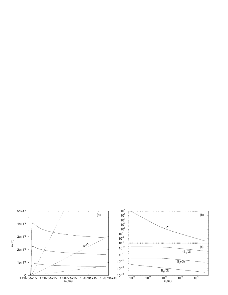
Figure 2.— Solution $b$, corresponding to $\tau=10^{-6}$, and $F=-1.9$. ($a$) Three field lines ($\Phi=0.25\,,1\,,4$ – dashed) and three current lines (solid). ($b$)–($c$) The Poynting-to-matter energy flux ratio $\sigma$ and the magnetic field components for the reference field line $\Phi=1$.

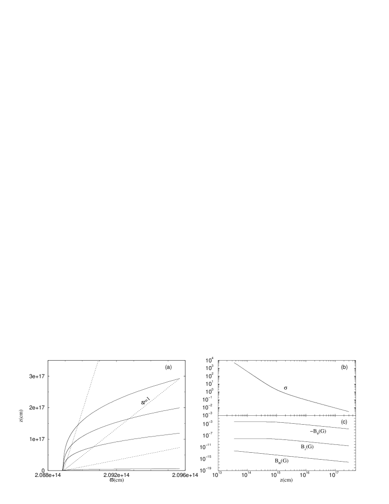
Figure 3.— Same as fig. 2, but for the solution $c$, corresponding to $\tau=10^{-5}$, and $F=-2.5$. Here $J_{\parallel}<0$ all the way from the origin to infinity, and there is no distributed return-current regime.

Besides the value of $\sigma_{\infty}$, another important issue is the acceleration rate. In this section we focus on the field line asymptotic shape in the regime $\sigma<1$ and its relation to the acceleration. (The analysis holds for nonrelativistic flows as well.) Note that the discussion of the present section – as well as the characteristics of the flow described in § 2.2.1 – is general and not restricted to the self-similar solutions presented in § 3. It applies in the asymptotic regime $\sigma<1$ where the motion is mainly poloidal, $V_{\phi}\ll V_{p}$. Equation (3b) yields $-\varpi B_{\phi}\propto\varpi^{2}B_{p}$, or, (using eq. [18]), $\sigma/(1+\sigma)\propto\varpi^{2}B_{p}$ (see also eq. [17a]). Thus, an accelerating flow corresponds to a decreasing $\varpi^{2}B_{p}$, a function that depends on the line shape. In other words, how fast the acceleration takes place depends on the magnetic flux distribution, by the solution of the transfield equation.

We already know that a field line shape of the form $z=c_{1}(A)\varpi^{c_{2}(A)}$ gives only logarithmic acceleration (Chiueh et al. 1991). The deviations from monopole magnetic field also result in inefficient (Beskin, Kuznetsova, & Rafikov, 1998), or logarithmic (Lyubarsky & Eichler, 2001) acceleration. (The monopole geometry itself – which however does not satisfy the transfield equation – gives extremely inefficient acceleration: $\sigma_{\infty}=\mu/\gamma_{\infty}=\mu^{2/3}\gg 1$; Michel, 1969.) The logarithmic acceleration gives asymptotically $\sigma_{\infty}=0$, but over completely unrealistic (exponentially large) distances. The numerical simulations by Bogovalov (2001) also give inefficient acceleration, possibly because the initial configuration is a split monopole field and does not change much during the simulation.

The $r$ self-similar solutions of Li et al. (1992) and Vlahakis & Königl (2003a) give final equipartition $\sigma_{\infty}=1$, but the same model could give smaller $\sigma_{\infty}$ as well (Vlahakis & Königl, 2003b; Vlahakis at al., 2003). However, because it cannot capture the transition from positive to negative curvature radius, it is impossible to obtain $\sigma_{\infty}=0$. The asymptotics of the $r$ self-similar model are straight poloidal field lines ($\varpi/{\cal R}=0$); as a result, the transfield component of the electromagnetic force asymptotically equals the “centrifugal” force (which could be very small, but definitely not exactly zero), and $\sigma_{\infty}=\sigma_{c}$. Even so, the value $\sigma_{c}$ could be very small, and the model should be explored more carefully in that respect.

In the $z$ self-similar model presented in § 3, we kept the line shape free: $z\propto\Phi(A)\zeta(\varpi)$, and the solution itself finds the shape through the function $\zeta(\varpi)$. The result is a quasi-conical shape, and the distribution of the magnetic flux is different from the monopole field (see eq. [23a]).

Table 1 Possible asymptotic geometries and the corresponding acceleration^†

	The far-asymptotic regime (after the end of the main acceleration)
	$\sigma\rightarrow 0$	$0<\sigma_{\infty}<\sigma_{c}$	$\sigma_{\infty}=\sigma_{c}$	$\sigma_{\infty}>\sigma_{c}$
	$I\rightarrow 0$	$I_{\infty}=I_{\infty}(A)\neq 0$	$I_{\infty}=I_{\infty}(A)\neq 0$	$I_{\infty}=I_{\infty}(A)\propto\gamma_{\infty}(A)^{*}$
	$f_{I\bot}=-f_{C\bot}$	$(f_{I\bot}=-f_{C\bot})_{\infty}$	$(f_{EM1}=-f_{C\bot})_{\infty}$	$(f_{EM1})_{\infty}=0$
	parabolic II or IIa	hyperbolic	conical I or Ia	conical I or Ia
The $\sigma_{c}<\sigma<1$ acceleration phase			or parabolic I or Ia	or parabolic I or Ia
$f_{EM1}=-f_{I\bot}$			or cylindrical	or cylindrical
conical Ia: $\ z=z_{0}(A)+{\varpi}/{\tan\vartheta(A)}$
$1/\varpi^{2}B_{p}={\vartheta^{{}^{\prime}}/\sin\vartheta-z_{0}^{{}^{\prime}}\sin\vartheta/\varpi}$	$\surd$	$\surd$	$\surd$	$\surd$
parabolic Ia: $\ z=z_{0}(A)+c_{1}(A)\varpi^{c_{2}}$, $c_{2}=$const
$1/\varpi^{2}B_{z}={(-c_{1}^{{}^{\prime}}/c_{1}c_{2})-(z_{0}^{{}^{\prime}}/c_{1}c_{2})\varpi^{-c_{2}}}$	$\surd$	$\surd$	$\surd$	$\surd$
parabolic II: $\ z=c_{1}(A)\varpi^{c_{2}(A)}$
$1/\varpi^{2}B_{z}={(-c_{1}^{{}^{\prime}}/c_{1}c_{2})-(c_{2}^{{}^{\prime}}/c_{2})\ln\varpi}$	$\surd$	$\surd$	—	—
parabolic IIa: $\ z=z_{0}(A)+c_{1}(A)\varpi^{c_{2}(A)}$
$1/\varpi^{2}B_{z}={(-c_{1}^{{}^{\prime}}/c_{1}c_{2})-(c_{2}^{{}^{\prime}}/c_{2})\ln\varpi-(z_{0}^{{}^{\prime}}/c_{1}c_{2})\varpi^{-c_{2}}}$	$\surd$	$\surd$	—	—
† The table covers the asymptotics of nonrelativistic flows as well.
∗ This is the solvability condition at infinity (Heyvaerts & Norman, 1989; Chiueh et al., 1991).

Collimation of relativistic outflows is in general much more difficult than in the nonrelativistic cases, firstly because the electric force almost cancel the transfield component of the magnetic force, and secondly because the effective matter inertia is larger (e.g., Bogovalov 2001). The result is negligible curvature, $\varpi/{\cal R}\approx 0$ (e.g., Chiueh, Li, & Begelman 1998), and only close to the origin where the Lorentz factor is smaller than a few tens is collimation efficient (Vlahakis & Königl, 2003b). This result, together with the envisioned close to $z=\varpi/\tan\vartheta(A)$ field line shape – we employ the term “type I conical” for this shape – led to the erroneous conclusion that acceleration is impossible when $\varpi/{\cal R}\approx 0$. However, negligible curvature does not necessarily mean $z\propto\varpi$; the most general case is a “type Ia conical” shape given by

$$z=z_{0}(A)+\frac{\varpi}{\tan\vartheta(A)},\quad z_{0}^{{}^{\prime}}\neq 0\,.$$ (34)

Differentiating equation (34) we get for the poloidal magnetic field

$$\varpi^{2}{\boldsymbol{B}}_{p}=\varpi{\boldsymbol{\nabla}}A\times\hat{\phi}=\frac{\cos\vartheta\ \hat{z}+\sin\vartheta\ \hat{\varpi}}{\vartheta^{{}^{\prime}}/\sin\vartheta-z_{0}^{{}^{\prime}}\sin\vartheta/\varpi}\,.$$ (35)

(Here primes denote derivative with respect to $A$.) It is evident from equation (35) that for $z_{0}^{{}^{\prime}}>0$, $\vartheta^{{}^{\prime}}>0$ the quantity $\varpi^{2}B_{p}$ is a decreasing function of $\varpi$, meaning that the flow is accelerated. Magnetic flux conservation implies $2\pi\delta A=B_{p}\delta S$, where $\delta S$ is the cross-section area between two neighboring magnetic flux surfaces $A$, $A+\delta A$ ($\delta S=2\pi\varpi\delta\ell_{\bot}$, see fig. 4). Since $B_{p}\varpi^{2}/\delta A=2\pi\varpi^{2}/\delta S$, it is clear that acceleration is possible when – as the flow moves – $\delta S$ increases faster than $\varpi^{2}$. This is the case in type Ia conical flow, while in type I conical it is exactly $\delta S\propto\varpi^{2}$ and the quantity $B_{p}\varpi^{2}$ remains constant. The previous analysis shows that the argument of Chiueh et al. (1998) related to the global inefficiency of the magnetic acceleration in relativistic flows (based on the fact that the collimation is inefficient), can be circumvented. The conical Ia field lines are perfectly straight, satisfying the $\varpi/{\cal R}=0$, nevertheless, they expand in the sense that $\delta S$ increases faster than $\varpi^{2}$. In other words, we may have expansion (increasing $\delta S/\varpi^{2}$), without bending ($\varpi/{\cal R}\neq 0$).
By combining equations (35) and (17a), we find that the $\sigma$ function could change from a $\sim 1$ value at $\varpi\sim Az_{0}^{{}^{\prime}}\sin\vartheta/(A\vartheta^{{}^{\prime}}/\sin\vartheta-2\sigma_{\rm M}/\mu)$ (the conical Ia shape starts roughly at this distance), and becomes $\sigma=\sigma_{\rm min}$ at distances $\varpi\gg z_{0}^{{}^{\prime}}\sin^{2}\vartheta/\vartheta^{{}^{\prime}}$, with

$$\sigma_{\rm min}=\frac{\sigma_{\rm M}}{\mu}\left(\frac{B_{p}\varpi^{2}}{A}\right)_{\rm min}=\frac{\sigma_{\rm M}}{\mu}\frac{\sin\vartheta}{A\vartheta^{{}^{\prime}}}\,.$$ (36)

Since the factor $\sin\vartheta/A\vartheta^{{}^{\prime}}$ is not $\ll 1$ (this would require the opening of the field lines asymptotically to change rapidly from line-to-line which is unlikely to happen) the only case that gives $\sigma_{\rm min}\ll 1$ is the $\mu\gg\sigma_{\rm M}$. This is an important requirement for the above mechanism to work, and it is equivalent to $B_{p}\varpi^{2}\gg A$ in the super-Alfvénic regime and as long as the $\sigma$ is $\gg 1$ [in this regime $\mu\approx-\varpi\Omega B_{\phi}/\Psi_{A}c^{2}\approx B_{p}\varpi^{2}\Omega/\Psi_{A}c^{3}=(B_{p}\varpi^{2}/A)\sigma_{\rm M}$]. Hence, as Chiueh et al. (1998) state, the poloidal field lines need to be bunched within a small solid angle before expansion takes place. Contrary to their claim, however, the expansion is not necessarily sudden near the light cylinder, but extended to $x\gg 1$. In § 5 we discuss how such a field configuration may be created (see also fig. 4).

The general asymptotic expansion of the field line configuration – in both, relativistic and nonrelativistic cases – is

$$z=z_{0}(A)+c_{1}(A)\varpi^{c_{2}(A)}\,,$$ (37)

for which we get

$$\varpi^{2}B_{z}=\varpi\frac{\partial A}{\partial\varpi}=\frac{c_{2}}{-c_{1}^{{}^{\prime}}/c_{1}-c_{2}^{{}^{\prime}}\ln\varpi-(z_{0}^{{}^{\prime}}/c_{1})\varpi^{-c_{2}}}\,.$$ (38)

Chiueh et al. (1991) examined two types of parabolic cases: type I ($z_{0}^{{}^{\prime}}=0\,,c_{2}\neq 1\,,c_{2}^{{}^{\prime}}=0$) when $\varpi^{2}B_{z}$ is a field line constant, and type II ($z_{0}^{{}^{\prime}}=0\,,c_{2}\neq 1\,,c_{2}^{{}^{\prime}}\neq 0$) when the $\varpi^{2}B_{z}$ slowly (logarithmically) decreases and asymptotically vanishes. They also examined the conical type I case ($z_{0}^{{}^{\prime}}=0\,,c_{2}=1$). Besides the conical type Ia case, new types of parabolic cases corresponding to $z_{0}^{{}^{\prime}}\neq 0$ should be added in the analysis. We henceforth call them type Ia, for $c_{2}=$const$\neq 1$, and type IIa, for $c_{2}=c_{2}(A)\neq 1$. These new parabolic types together with the type Ia conical, are much faster than logarithmic accelerators in relativistic as well as in nonrelativistic flows. Table 1 summarizes the various possible geometries in the acceleration phase $\sigma_{c}<\sigma<1$ (first column) combined with the possible final results of the acceleration – including possible acceleration after the $\sigma=\sigma_{c}$ transition – and the far-asymptotic final geometries. The final current distribution and the dominant forces in the transfield direction are also shown. Compatible combinations of the geometry in the acceleration phase $\sigma_{c}<\sigma<1$ and the far-asymptotic final state are marked with a “$\surd$”. For example, if the flow has a type Ia conical shape (this is the most plausible case for relativistic MHD in which the field lines have negligible curvature $\varpi/{\cal R}\ll 1$), the $\sigma$ function decreases according to equation (17a) and the shown in the Table 1 function $\varpi^{2}B_{p}$, and reaches a minimum value $\sigma_{\rm min}$ at distances $\varpi\gg z_{0}^{{}^{\prime}}\sin^{2}\vartheta/\vartheta^{{}^{\prime}}$ (see eq. [36]). If the azimuthal centrifugal force is still negligible at these distances (i.e., $\sigma_{\rm min}>\sigma_{c}$) the acceleration stops and the far-asymptotic regime is the one in the fifth column (most likely with unchanged conical Ia shape). If $\sigma_{\rm min}\approx\sigma_{c}$, then the azimuthal centrifugal force starts to play a role in determining the poloidal curvature. One possibility is that the acceleration does not continue even with slightly different line shape, resulting in the fourth column case. The remaining case is that the $\sigma$ continues to decrease, and the line shape becomes hyperbolic. Since the asymptotic form of a hyperbolic flow is again conical, the $\sigma$ function reaches a new minimum given from an equation similar to (36). If the acceleration stops at this point, we get a final situation corresponding to the third column of Table 1. However, even tiny deviations from an exactly radial flow $\varpi/{\cal R}=0$ could give a slow (logarithmic) acceleration to the completely matter-dominated regime $\sigma_{\infty}=0$, as was argued by Okamoto (2002). This situation corresponds to a continuous acceleration under a parabolic II or IIa shape (second column). We note, however, that for realistic applications, the interaction of an outflow with its environment brakes-down the ideal MHD conditions and this probably happens before the realization of this last part of the acceleration.

Chiueh et al. (1991) examined the far-asymptotics of relativistic MHD outflows, generalizing the work on nonrelativistic flows by Heyvaerts & Norman (1989). They assumed that the various quantities become functions of $A$ alone (the characteristic of the far-asymptotic regime), neglected the poloidal centrifugal term ${\cal O}(\varpi/{\cal R})$ as well as terms of order ${\cal O}(x_{\rm A}^{2}/x^{2})$ in the transfield equation, and found that conical field lines satisfying $(z/\varpi)_{\infty}<\infty$ should enclose a finite current $I_{\infty}=I_{\infty}(A)\propto\gamma_{\infty}(A)$ (the solvability condition at infinity, see §2.2.1). As already discussed in §2.2.1, this is the case when $\sigma_{\infty}>\sigma_{c}$, but for smaller values of $\sigma_{\infty}$ the asymptotic transfield equation reduces to the balance between the poloidal and azimuthal centrifugal forces [i.e., they are exactly the ${\cal O}(x_{\rm A}^{2}/x^{2}),{\cal O}(\varpi/{\cal R})$ terms that remain in the transfield]; the electromagnetic term is much smaller, but nevertheless not exactly zero and no solvability condition can be derived. Our self-similar solutions fall in this category: the condition $I_{\infty}(A)\propto\gamma_{\infty}(A)$ is not satisfied, because $\sigma_{\infty}<\sigma_{c}$.

As we see in Table 1 the solvability condition at infinity is mandatory only for the fifth column. As a result we may have, e.g., nonrelativistic conical or type I/Ia parabolic flows that carry poloidal current $I_{\infty}=I_{\infty}(A)$ (with negative or positive $dI_{\infty}/dA$ when they are in the current-carrying or return-current regime respectively), provided that $\sigma_{\infty}\leq\sigma_{c}$.

As we already stated, the analysis of this section applies to nonrelativistic flows as well. A first step towards finding nonrelativistic MHD solutions with $\sigma_{\infty}\approx 0$ is the super– modified fast-magnetosound solution of Vlahakis et al. (2000), which ends slightly after the modified fast singular point with $\sigma=0.005$. The full acceleration ($\sigma_{\infty}=0$) should be examined using a model that allows a transition from positive to negative curvature radius (the asymptotic transfield force-balance equation for nonrelativistic flows implies that the curvature radius has the sign of the $-J_{\parallel}$, thus changing sign when the flow moves from the current-carrying to the return-current regime, e.g., Okamoto, 2001).

5. The pulsar magnetosphere/equatorial wind

The most efficient acceleration mechanism that we described is the one based on the conical Ia field line shape. The $z$ self-similar solutions are just a numerical example confirming that the mechanism indeed works. Although the presented solutions describe an outflow very close to the polar axis, the same exactly physical mechanism is expected to work for the equatorial wind as well. Only practical difficulties do not allow us to derive semianalytical solutions in that regime.

As we discuss in § 4, an important requirement for the above mechanism to work is that $\mu\gg\sigma_{\rm M}$. In fact, as we argue below, such a configuration is most likely to happen near the equator.

The pulsar magnetosphere has been traditionally considered as being force-free, and inertial effects are usually neglected. On the other hand, it is generally accepted that it is because of the inertia that the magnetic field line topology becomes open and an azimuthal magnetic field component is created. Moreover, the pair creation and their acceleration to high Lorentz factors (e.g., Daugherty & Harding 1982) involve non-ideal MHD effects that may be important in the final form of the magnetosphere. A question arises: is the force-free a good approximation?

Contopoulos et al. (1999) have solved the force-free problem (although with the current-closure not fully satisfied) and Ogura & Kojima (2003) have repeated their numerical work with higher resolution, deriving similar results. The usual problem with the force-free dynamics is that the condition $B^{2}-E^{2}>0$ is not always satisfied, since the Bernoulli equation that relates the electromagnetic field with the Lorentz factor of the system of reference where the electric field vanishes, is omitted (see eq. [12]). In regimes where $B^{2}<E^{2}$ the drift velocity is larger than the light speed. This is indeed the case in the aforementioned force-free solution. According to Ogura & Kojima (2003) the drift velocity becomes larger than the light speed at distance a few times the light cylinder (their figure 5 shows that typically this happens at cylindrical distance $\approx 3c/\Omega$). Thus, the force-free assumption brakes-down much before the fast-magnetosound point ($\sigma=\mu^{2/3}$).

Another problem of the force-free solution is that it implies negative azimuthal velocities near the source. Contopoulos et al. (1999) demonstrated how we can find the flow speed in cases where the electromagnetic field is known. We need to solve the system of equations (coming from eq. [3b], and the second of eqs. [5d])

$$\frac{V_{\phi}}{cx}=1-\frac{V_{p}}{c}\frac{2|I|}{\Omega B_{p}\varpi^{2}}\,,$$ (39a)

$$\xi\gamma\left(1-x\frac{V_{\phi}}{c}\right)=\mu(1-x_{\rm A}^{2})\,,$$ (39b)

together with the identity $1-1/\gamma^{2}=(V_{p}/c)^{2}+(V_{\phi}/c)^{2}$. The solution for $\gamma$ is actually equation (12). The problem related to negative azimuthal speeds comes from equation (39a). The second part of the right-hand side is much smaller than unity very close to the source in a possible corotating regime, and should increase up to an asymptotic value equal to unity as we move to larger $x$ (in order to have a negligible asymptotic azimuthal speed). Practically speaking, the ratio $2|I|/\Omega B_{p}\varpi^{2}$ should be $\approx 1$ at distances $x\gtrsim$ a few. After that point $\left(B_{p}\varpi^{2}\right)_{x>\mbox{a few}}\approx 2|I|/\Omega$, and this continues to be the case even in the superfast (non-force-free) regime where both the $|I|$ and the $B_{p}\varpi^{2}$ decrease. But, what happens relatively close to the light cylinder? The poloidal field lines follow the dipolar shape up to the point where they approach the equator, but then they remain parallel to it for some distance. We know that a relativistic flow is difficult to bend and this is a characteristic of a force-free regime as well. The curvature $1/{\cal R}$ is of the order of $(1/z)\times{\cal O}\left({{\rm max}}\{1/x^{2}\,,1/\gamma^{2}\}\right)$, meaning that at distances $x\gtrsim$ a few, the poloidal field lines are practically straight. As a result, the quantity $\varpi^{2}B_{p}$ increases, because the surface between two neighboring field lines increases slower that $\propto\varpi^{2}$. For a force-free case where $|I|$ remains constant, we get a decreasing ratio $(V_{p}/c)(2|I|/\Omega B_{p}\varpi^{2})$. Since its asymptotic value should be unity, near the source is larger than unity, implying $V_{\phi}<0$. In fact Contopoulos et al. (1999) found negative azimuthal velocities. The only way to avoid this effect in the framework of force-free field, is to have very small initial poloidal velocity ($V_{p}\ll c$), meaning that our “initial” surface is very close to the pulsar. However, in that case we should take into account non-ideal effects related to the pair creation region.

A solution to this problem could be that the flow in the regime where the lines remain approximately parallel to the equator is decelerating, meaning that kinetic (or enthalpy) energy flux is transfered to Poynting, and the $\sigma$ function increases. In that case, the $|I|=(c/2)\varpi|B_{\phi}|$ would increase and cancel the increase of $B_{p}\varpi^{2}$ in the expression of $V_{\phi}$, resulting in $V_{\phi}>0$. During the phase where the flow is approximately parallel to the equator, the $B_{p}\varpi^{2}=\delta A(2\pi\varpi^{2})/\delta S$ increases almost linearly with $\varpi$ ($\delta S\approx 2\pi\varpi\delta z$ with $\delta z\approx const$). Since the $\varpi|B_{\phi}|$ is forced to follow this increase (in order to be consistent with a negligible azimuthal motion), the matter energy part is decreasing linearly with $\varpi$, and an important (or even the most significant) part of the Poynting flux may be created there. As the flow decelerates, at some point it reaches $\gamma\sim 10$. Only after that point the curvature of the poloidal field lines $(1/{\cal R})$ may be important and the lines start to expand to larger heights above the equator. The expansion in principle allows for acceleration (if $\delta S$ increases faster than $\varpi^{2}$), and this time the electromagnetic energy is transfered to the matter. We consider this point as the origin of the ideal MHD regime that we examine in this paper.

Another problem comes when we consider the “last” current loop ($I=0$) that closes on the equator. Along this equatorial current line the azimuthal magnetic field vanishes. Since $B^{2}-E^{2}=B_{\phi}^{2}-B_{p}^{2}(x^{2}-1)$, the inequality $B^{2}-E^{2}>0$ holds only in the unlikely case where the poloidal field also vanishes on the equator. The remaining case is to include non-ideal MHD effects (then the electric field is not equal to $xB_{p}$ and $B^{2}-E^{2}=B_{p}^{2}-E^{2}$ could be positive).

Although the details of the full magnetosphere remain to be explored, and this requires to solve the full problem (not only the non-force-free, but also the non-ideal MHD especially near the “last” current line that closes on the equator; not to mention the inner/outer gaps and the non-axisymmetry), the picture described above looks appealing and consistent with the observed Crab-pulsar equatorial wind. The scenario also explains why the quantities $B_{p}\varpi^{2}/A$, $2|I|/A\Omega\approx\mu/\sigma_{\rm M}$, and $1/\sigma$ are likely $\gg 1$ just after the end of this “parallel to the equator” phase. These are the “initial” conditions for the ideal MHD phase. It may not be just a coincidence that the efficient and faster than logarithmic acceleration to low-$\sigma$ values during the ideal MHD phase was possible for these “initial” conditions only. Note also that the part of the total open magnetic flux that contributes to the “parallel to the equator” phase, is $\sim 50\%$ (for exactly dipolar field, $45\%$ of the open magnetic flux correspond to field lines that have $B_{z}<0$ when cross the light cylinder). The rest $\sim 50\%$ of the open field lines likely follows a dipolar shape till $x\sim$ a few, and then becomes conical Ia (again $\varpi/{\cal R}$ is negligible). Since there is no obvious reason for an increasing $B_{p}\varpi^{2}$, the acceleration gives asymptotically $\sigma_{\infty}\sim 1$ or $\sigma_{i}$, if the initial $\sigma$ value is $\sigma_{i}\gg 1$ or $\sigma_{i}\ll 1$, respectively.

The “initial” conditions $B_{p}\varpi^{2}\gg A$ are in principle possible in other astrophysical settings as well, such as gamma-ray burst sources or AGNs. For example, a corona or a thermal/radiation pressure field may keep the field lines that emanate from a disk parallel to each other (at least for some distance), in which case the product $B_{p}\varpi^{2}$ again increases and a matter energy-to-Poynting flux transformation is realized (e.g., Vlahakis & Königl, 2003b; Vlahakis at al., 2003).

6. Summary

In the first part of the paper (§ 2.1, 2.2) we derived the ideal MHD equations that describe the super-Alfvénic asymptotic regime. The resulting system of equations remains intractable enough, and we could only find a $z$ self-similar model (§ 3) describing the regime near the rotation axis. We regard the solution $a$ as the best representative result of that model. It includes all the expected characteristics of an efficient MHD accelerator, in particular:

• The transition from $\sigma=10^{4}$ to $\sigma\approx 0$, showing that ideal MHD can account for the full acceleration, resulting in a matter-dominated flow.

• The transition from a current-carrying to a return-current regime, showing how the poloidal current lines close.

• The transition from positive to negative poloidal curvature radius. When the flow becomes sufficiently matter-dominated ($\sigma<\sigma_{c}$; see §2.2.1) it has a negative curvature radius and the line shape becomes hyperbolic. This is simply the result of angular momentum conservation: the azimuthal component of the velocity decreases, and the constancy of the total velocity implies an increasing cylindrical component. (This small deviation from a conical line shape could be enhanced in the termination shock.) The most important implication of this effect is not the hyperbolic line shape itself (which still remains practically conical), but the new status quo in the transfield force-balance. It is now the poloidal and azimuthal centrifugal inertial forces that dominate and their difference is the much smaller transfield electromagnetic force component.

• The transition from sub– to super– modified fast-magnetosound flow. This surface should be crossed since in the matter-dominated regime the fast-magnetosound speed becomes progressively smaller (it vanishes at $\sigma=0$). In this sense it is a signature of an efficient acceleration. It is also related to the causality principle: only in the super– modified fast-magnetosound regime none of the MHD waves can propagate upstream and reach the origin of the flow.

We tried to present our numerical solutions in accord with the model of Kennel & Coroniti for the Crab nebula. In solution $a$ the transition from $\sigma=10^{4}$ to $\sigma_{s}=0.003$ happens over less than five decades in distance from the pulsar, and the value $\sigma_{s}$ is reached at distance of $3\times 10^{17}$cm. As we discussed in §3.1.1, $\sigma$ decreases as $\propto 1/z$ in the non-force-free regime $\sigma<$ a few (and even faster when $\sigma>$ a few).

The assumption $B_{z}\gg B_{\varpi}$ – required in order to derive the $z$ self-similar model – does not allow us to examine the wind near the equator. Nevertheless, the presented numerical solutions serve as the first examples of low-$\sigma$ asymptotic flows, and, more importantly, they guided us to think which is the situation in the most general (non-self-similar) case. Our main conclusions (described and justified in § 2.2.1 and §4) are in summary:

• Type Ia conical flows (eq. [34]) are efficient accelerators. The $\sigma$ decreases much faster than logarithmically.

• The same for the parabolic Ia, IIa (they likely apply to nonrelativistic flows).

• For sufficiently small asymptotic values of the $\sigma$ function, a transition $\sigma=\sigma_{c}$ exist, where the azimuthal centrifugal force is comparable to the electromagnetic force in the transfield direction. The acceleration may or may not continue after this transition. In both cases, however, the solvability condition at infinity (Heyvaerts & Norman 1989; Chiueh et al. 1991) is not mandatory. The latter should be satisfied only in cases where $\sigma_{\infty}>\sigma_{c}$. Note that for the equatorial pulsar wind the ratio $f_{EM1}/f_{C\bot}\sim\sigma x^{2}/\gamma^{2}$ is $\gg 1$ at the position of the shock (for $\sigma\approx 0.003$, $x\sim 10^{9}$, and $\gamma\approx 10^{6}$). However, the solvability condition may not be satisfied, if the value of the $\sigma$ required at the shock is not the asymptotic $\sigma_{\infty}$, but the $\sigma$ function still decreases at the position of the shock. Moreover, in applications to jets related to other astrophysical settings, the transition $\sigma=\sigma_{c}$ may be important.

• In flows where the acceleration continues to $\sigma<\sigma_{c}$, the line shape is hyperbolic and the curvature radius of the poloidal field-streamlines becomes negative.

A required condition for the above acceleration mechanism to work is $\mu\gg\sigma_{\rm M}$. As we discuss in § 4, this condition means that at the inner super-Alfvénic regime $B_{p}\varpi^{2}$ should be $\gg A$, and the current that flows along the field lines should be much larger than the typical values obtained in monopole solutions, $|I|\gg A\Omega$. We argue in § 5 that this condition is likely satisfied for the equatorial wind. The scenario presented in that section is outlined below with the help of the figure 4. The various transitions/regimes as we move along the reference (thicker) field line, marked with the numbered vertical dotted lines are:

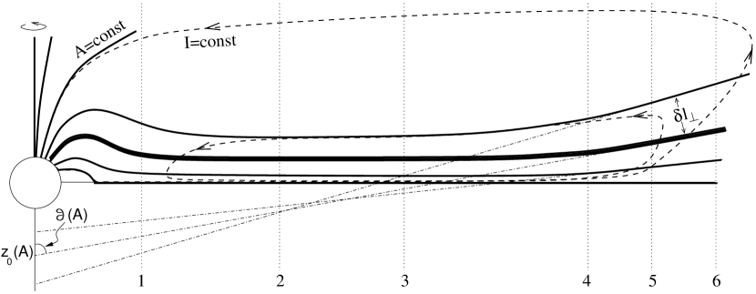
Figure 4.— Sketch of an equatorial pulsar wind (not in scale). The lines of the poloidal magnetic field – the $A=const$ bold lines – have a dipolar shape close to the source and after a phase where they are roughly parallel to the equator (bunched within a small solid angle), they become type conical Ia [$z=z_{0}(A)+\varpi/\tan\vartheta(A)$]. The lines of the poloidal current $\boldsymbol{J}_{p}$ – the $I=const$ dashed lines – are also shown. The various transitions/regimes marked with the numbered vertical dotted lines are discussed in § 6.

– Origin $\rightarrow$ 1: This is the most uncertain regime, and very important problem for future research. We can only speculate what may happen there. The poloidal field possibly starts with a dipolar shape, however, inertial effects (associated with the azimuthal velocity) create an open magnetosphere. (Note that even under force-free conditions the last closed field line does not in principle intersect the equator at the light cylinder; see Uzdensky, 2003). Non-ideal MHD effects accelerate created pairs to $\gamma_{1}\gg 1$. One has to solve the dynamics by including the back-reaction from the various emission mechanisms to yield the exact value of $\gamma_{1}$. In principle, this value could correspond to matter-dominated flow $\sigma_{1}\ll 1$ (although the poloidal field is strong, the Poynting flux associated with the $EB_{\phi}$ product may not be larger than the matter energy flux). The initial conditions after the pair acceleration in the non-ideal MHD regime may correspond even to super-Alfvénic conditions in which case the light cylinder has not a particular physical meaning.
– 1: Here $x\sim$ a few. This may be the base of the ideal MHD regime (although there should be non-ideal effects near the midplane even after that point, see § 5). Downstream from this point the super-Alfvénic asymptotic analysis holds. According to equation (13), $xB_{p}\approx(-B_{\phi})(1-1/2\gamma^{2}+1/2x^{2})\approx-B_{\phi}$, and $|I|=(c/2)\varpi|B_{\phi}|\approx(\Omega/2)B_{p}\varpi^{2}$. Also the poloidal curvature is $\varpi/{\cal R}\ll 1$ and the poloidal field lines are approximately straight and roughly parallel to the equator.
– 1 $\rightarrow$ 2: The product $B_{p}\varpi^{2}$ increases as $2\pi\varpi^{2}\delta A/\delta S=\varpi\delta A/\delta l_{\bot}$, where $\delta l_{\bot}$ is the distance between two neighboring field lines $A$, $A+\delta A$ (see fig. 4). Since the $\varpi E\propto B_{p}\varpi^{2}$ increases, $|I|=(c/2)\varpi|B_{\phi}|$ should also increase in order to keep the inequality $B^{2}>E^{2}$ true. Thus, matter kinetic energy (and possibly thermal energy) is transfered to Poynting. Figure 4 shows a current loop that crosses the reference field line between points 1 and 2. Here $J_{\bot}<0$ and the associated Lorentz force $(c/4\pi)J_{\bot}B_{\phi}$ decelerates the matter, increasing the $\sigma$ function. Also $J_{\parallel}<0$, $J^{0}<0$, but the transfield component of the Lorentz force [$f_{B\bot}+f_{E\bot}\approx(c/4\pi)(J^{0}E+J_{\parallel}B_{\phi})$] remains small, resulting in $\varpi/{\cal R}={\cal O}\left({{\rm max}}\{1/x^{2}\,,1/\gamma^{2}\}\right)$, (e.g. Chiueh et al., 1998).
– 2: Here the Lorentz factor is sufficiently small ($\lesssim 10$) for the field lines to start slightly bending. This is the base for the accelerating ideal MHD regime described in the previous sections. This point corresponds to an “initially” Poynting flux-dominated wind. The “initial” conditions satisfy $B_{p}\varpi^{2}=(B_{p}\varpi^{2})_{i}\gg A\Leftrightarrow\mu\gg\sigma_{\rm M}$ and the $\sigma$ function is $\gg 1$.
– 2 $\rightarrow$ 4: The field lines have a parabolic shape: $\delta l_{\bot}/\varpi\delta A$ slightly increases, resulting in a tiny decrease in $B_{p}\varpi^{2}$. The $\sigma$ function decreases according to the equation (17a). For the poloidal current density, $J_{\parallel}<0$, $J_{\bot}>0$.
– 3: Classical fast-magnetosound point, $\gamma_{3}\approx\mu^{1/3}$, $\sigma_{3}\approx\mu^{2/3}$.
– 4: The $\sigma$ function is unity. Equation (17a) implies that $B_{p}\varpi^{2}=(B_{p}\varpi^{2})_{i}/2$.
– 4 $\rightarrow$ 6: This is the conical Ia phase (the discussion of § 4 refers to this regime). The field lines become $z=z_{0}(A)+\varpi/\tan\vartheta(A)$ (tangent to the dot-dashed lines in fig. 4). It is seen in figure 4 how the conditions $z_{0}^{{}^{\prime}}>0$, $\vartheta^{{}^{\prime}}>0$ are realized. The $B_{p}\varpi^{2}$ decreases according to equation (35). As a result, the $\sigma$ function decreases from $\approx 1$ to $\sigma_{\rm{min}}$ given by equation (36).
– 5: The current loop that the reference field line crosses at this point has $J_{\parallel}=0$, i.e., here the current-carrying regime ($J_{\parallel}<0$) ends and the return-current regime begins ($J_{\parallel}>0$).
– 6: Here the $B_{p}\varpi^{2}/A$ is of the order of unity. The fast acceleration cannot continue after that point. However, due to a tiny deviation from a $\varpi/{\cal R}=0$ it may continue logarithmically (see Chiueh et al., 1998 and references therein).

If at point 6 the value of $\sigma_{6}$ is $\sigma_{s}=0.003$ while at point 2 the flow is Poynting dominated ($\sigma_{2}\gg 1$), then the ratio $(B_{p}\varpi^{2})_{6}/(B_{p}\varpi^{2})_{2}=\sigma_{6}$ and the required value for the $B_{p}\varpi^{2}/A$ at point 2 is $1/\sigma_{6}\approx 300$. Assuming further that ideal MHD holds during the 1 $\rightarrow$ 2 phase and that the flow started at 1 with $\sigma_{1}\ll 1$, we get $(B_{p}\varpi^{2})_{2}/(B_{p}\varpi^{2})_{1}=(B_{\phi}\varpi)_{2}/(B_{\phi}\varpi)_{1}=1/\sigma_{1}$. Thus, $(B_{p}\varpi^{2})_{1}/A=\sigma_{1}/\sigma_{6}\approx 300\sigma_{1}$. For a dipolar field before the point 1, $(B_{p}\varpi^{2})_{1}/A=2$, and we get a required value for $\sigma_{1}=2\sigma_{6}\approx 0.006$. However, it is not clear that all the above assumptions hold, so we cannot be sure for the derived value $\sigma_{1}$.

In general, the fast (faster than logarithmic) acceleration in magnetized outflows gives asymptotically $\sigma_{\rm min}\sim A/B_{p}\varpi^{2}=\sigma_{\rm M}/\mu$, where $B_{p}\varpi^{2}$ is the “initial” value at the Poynting dominated regime (point 2 in fig. 4). Besides the application to pulsar winds on which we focussed in this paper, the formulation presented is quite general and AGN or GRB relativistic as well as YSO nonrelativistic jet asymptotics can also be considered (the asymptotic analysis presented in § 2 applies in all these cases, no matter if asymptotically $\sigma\ll 1$ or $\sim 1$, or even $>1$). In addition, the $z$ self-similar model of § 3 could be used for examining AGN or GRB jets in their super-Alfvénic regime.

References

- Arons (1998) Arons, J. 1998, Mem. Soc. Astron. Italiana, 69, 989
- Arons (2002) Arons, J. 2002, in ASP Conf. Ser. 271, Neutron Stars in Supernova Remnants, ed. P. O. Slane & B. M. Gaensler (San Francisco: ASP), 71
- Begelman (1998) Begelman, M.C. 1998, ApJ, 493, 291
- Beskin, Kuznetsova, & Rafikov (1998) Beskin, V. S., Kuznetsova, I. V., & Rafikov, R. R. 1998, MNRAS, 299, 341
- Blandford (2002) Blandford, R. D. 2002, in Lighthouses of the Universe, ed. M. Gilfanov et al. (Berlin: Springer), 381
- Bogovalov (1997) Bogovalov, S. V. 1997, A&A, 323, 634
- Bogovalov (2001) Bogovalov, S. V. 2001, A&A, 371, 1155
- Bogovalov & Khangoulian (2002) Bogovalov, S. V., & Khangoulian, D. V. 2002, MNRAS, 336, L53
- Camenzind (1986) Camenzind, M. 1986, A&A, 162, 32
- Chiueh et al. (1991) Chiueh, T., Li, Z.-Y., & Begelman, M.C. 1991, ApJ, 377, 462
- Chiueh et al. (1998) Chiueh, T., Li, Z.-Y., & Begelman, M.C. 1998, ApJ, 505, 835
- Contopoulos (1995) Contopoulos, J. 1995, ApJ, 450, 616
- Contopoulos et al. (1999) Contopoulos, J., Kazanas, D., & Fendt, C. 1999, ApJ, 511, 351
- Contopoulos & Kazanas (2002) Contopoulos, J., & Kazanas, D. 2002, ApJ, 566, 336
- Daugherty & Harding (1982) Daugherty, J. K., & Harding, A. K. 1982, ApJ, 252, 337
- Gaensler et al. (2002) Gaensler, B. M., Arons, J., Kaspi, V. M., Pivovaroff, M. J., Kawai, N., & Tamura, K. 2002, ApJ, 569, 878
- Helfand, Gotthelf, & Halpern (2001) Helfand, D. J., Gotthelf, E. V., & Halpern, J. P. 2001, ApJ, 556, 380
- Heyvaerts & Norman (1989) Heyvaerts, J., & Norman, C. 1989, ApJ, 347, 1055
- Hester et al. (1995) Hester, J. J. et al. 1995, ApJ, 448, 240
- Kennel & Coroniti (1984a) Kennel, C. F., & Coroniti, F. V. 1984a, ApJ, 283, 694
- Kennel & Coroniti (1984b) Kennel, C. F., & Coroniti, F. V. 1984b, ApJ, 283, 710
- Königl & Granot (2002) Königl, A. & Granot, J. 2002, ApJ, 574, 134
- Li et al. (1992) Li, Z.-Y., Chiueh, T., & Begelman, M.C. 1992, ApJ, 394, 459
- Lyubarsky & Eichler (2001) Lyubarsky, Y., & Eichler, D. 2001, ApJ, 562, 494
- Michel (1969) Michel, F. C. 1969, ApJ, 158, 727
- Ogura & Kojima (2003) Ogura, J. & Kojima, Y. 2003, Progress of Theoretical Physics, 109, 619
- Okamoto (2001) Okamoto, I. 2001, MNRAS, 327, 55
- Okamoto (2002) Okamoto, I. 2002, ApJ, 573, L31
- Rees & Gunn (1974) Rees, M. J., & Gunn, J. E. 1974, MNRAS, 167, 1
- Stappers et al. (2003) Stappers, B. W., Gaensler, B. M., Kaspi, V. M., van der Klis, M., & Lewin, W. H. G. 2003, Science, 299, 1372
- Tomimatsu & Takahashi (2003) Tomimatsu, A. & Takahashi, M. 2003, ApJ, 592, 321
- Tsinganos et al. (1996) Tsinganos, K., Sauty, C., Surlantzis, G., Trussoni, E., & Contopoulos, J. 1996, MNRAS, 283, 811
- Uzdensky (2003) Uzdensky, D. A. 2003, ApJ, in press (preprint, astro-ph/0305288)
- Vlahakis & Tsinganos (1998) Vlahakis, N., & Tsinganos, K. 1998, MNRAS, 298, 777
- Vlahakis et al. (2000) Vlahakis, N., Tsinganos, K., Sauty, C., & Trussoni, E. 2000, MNRAS, 318, 417
- Vlahakis & Königl (2003a) Vlahakis, N., & Königl, A. 2003a, ApJ, 596, 000
- Vlahakis & Königl (2003b) Vlahakis, N., & Königl, A. 2003b, ApJ, 596, 000
- Vlahakis at al. (2003) Vlahakis, N., Peng, F., & Königl, A. 2003, ApJ, 594, L000