Constraints on AGN accretion disc viscosity derived from continuum variability

Abstract

We estimate a value of the viscosity parameter in AGN accretion discs for the PG quasar sample. We assume that optical variability on time-scales of months to years is caused by local instabilities in the inner accretion disc. Comparing the observed variability time-scales to the thermal time-scales of $\alpha$-disc models we obtain constraints on the viscosity parameter for the sample. We find that, at a given $L/L_{\rm Edd}$, the entire sample is consistent with a single value of the viscosity parameter, $\alpha$. We obtain constraints of $0.01\leq\alpha\leq 0.03$ for $0.01\leq L/L_{\rm Edd}\leq 1.0$. This narrow range suggests that these AGN are all seen in a single state, with a correspondingly narrow spread of black hole masses or accretion rates. The value of $\alpha$ we derive is consistent with predictions by current simulations in which MHD turbulence is the primary viscosity mechanism.

1 Introduction

The transport of angular momentum remains a major unknown in accretion disc theory. Shakura & Sunyaev (1973) suggested that magnetic fields and turbulent motions are likely candidates for the angular momentum transport. They argued that turbulence is a dominant factor and postulated that the stress is proportional to the local pressure. The proportionality parameter $\alpha$, which parametrizes the underlying transport process, describes the efficiency of the turbulent transport. The $\alpha$-parameter also represents the scale of the largest possible turbulent cell. The $\alpha$ parameterization provided a base for developing the accretion disc theory and linked the theory with the observations.

More recent work has shown that in weakly magnetized discs MHD turbulence can provide the majority of the outward transport of angular momentum (Balbus & Hawley, 1991). Balbus & Papaloizou (1999) reviewed the $\alpha$-disc models and found that MHD turbulence follows the $\alpha$ prescription very closely. They show that the vertically averaged disc with viscosity due to magnetorotational instabilities is described by a similar set of radial equations to the $\alpha$-discs. In particular the local energy dissipation rate is determined by the global disc parameters as it is in the $\alpha$-discs. However, global 3-D numerical simulations of accretion discs are extremely complex (Matsumoto & Shibata, 1997) and so most work to date has been done using local 2-D shearing box, cylindrical and axisymmetric limit models. All these methods have provided predictions of the $\alpha$-parameter ranging from $\sim$0.005 (Brandenburg et al. , 1995) to $\sim$0.6 (Hawley, Gammie & Balbus, 1995).

In order to determine the magnitude of the viscosity better estimates from larger samples of all categories of accreting objects are needed with independent methods for estimating $\alpha$. Since the spectrum of a disc at any particular instant is not strongly dependent on its viscosity the most effective way to estimate the viscosity is through the variability of the disc luminosity. A number of studies of this kind have been done for accreting binary systems since the time-scales of variability are optimal for observation, generally ranging from days down to a fraction of a second.

In the case of AGN we observe typical optical fluctuation time-scales of weeks to years although there have been only a few long-term monitoring programs to provide such data (eg. Pica et al. 1988; Giveon et al. 1999, hereafter G99). At optical and ultraviolet frequencies the majority of the continuum luminosity seen in AGN is held to be emission from the accretion disc (Malkan & Sargent, 1982) and large variability has been observed in these wavebands for many such objects (Webb & Malkan, 2000). The physical origin of optical flux variations has not been pinned down, but if disc emission dominates the spectrum at optical wavelengths the variability is expected to be related to the disc instabilities.

In this study we use a subset of the Palomar Green sample of AGN (G99), spanning approximately seven years of data, to derive limits on the viscosity parameter for the the sample as a whole via the method described in Siemiginowska & Czerny (1989, hereafter SC89). We assume any fluctuations in the lightcurves are due to an instability arising in the innermost disc regions and can be associated with the thermal time-scale. We do not identify the exact physical process responsible for this instability. It can be related to the Lightman-Eardley instabilities in the radiation pressure dominated region of the disc (Lightman & Eardley, 1974), but our method does not require modelling of the instability and therefore could be applied to any type of instability which may be present in the inner disc. Using a set of multi-temperature blackbody disc models, based on the standard $\alpha$-disc as prescribed by Shakura & Sunyaev (1973), we calculate the contribution to the optical spectrum from the outer, stable disc and assume that there is no contribution from the innermost parts of the disc where the instability has developed. Comparing the variability time-scales of the sources with the thermal time-scales of the models allows us to constrain the $\alpha$-parameter for the sample.

2 Data Sample

The data are taken from the optically selected Palomar-Green (PG; Schmidt & Green 1983) sample. A subset of 42 bright ($-28<M_{B}<-22$) and nearby AGN $(0.06<z<0.37)$ in the northern hemisphere were observed at the Wise Observatory, Israel (G99) in 1991-1998. Observations were made with a CCD camera mounted on the 1m optical telescope and span 7 years with a typical sampling interval of 39 days - a higher, more even sampling interval than that of previous programs (eg. Pica et al. 1988). The wavelength range covers the Johnson B band, 3600-5600 Å ($\lambda_{\rm central}$ = 4400 Å), which is a region of the spectrum believed to be dominated by the disc emission. The PG sample is statistically complete with good photometric accuracy over this wavelength range ($\sim$0.02 mag. at 4400 Å). G99 assume a Hubble constant $H_{0}$ = 70 kms^-1Mpc^-1, a deceleration parameter of $q_{0}$ = 0.2 and a power-law shaped continuum, $F_{\nu}\propto\nu^{-\alpha}$ where the spectral index $\alpha$ = 0.5 for the K-correction. This is a flux-limited sample so we expect to see selection effects as discussed in Schmidt & Green (1983). This sample has also been studied at a number of other wavelengths including R band (G99), radio (Kellermann et al. , 1989), IR (Neugebauer et al. , 1987) and X-ray (Laor et al. , 1997) and its optical polarization properties were studied by Berriman et al. (1990). Measurements of the masses of 17 PG quasars included in this subsample have been made by reverberation mapping (Kaspi et al. , 2000).

From the lightcurves we derived a two-folding time-scale as a characteristic time-scale for each source. The two-folding time-scale gives the time for an objects’ luminosity to change by a factor of two (either an increase or a decrease) which can be used as a measure of variability in both the data and the models (O’Brien, Gondhalekar & Wilson 1988 and references therein; SC89).

$$\tau_{\rm 2}=\tau_{\rm s}\frac{f_{\rm min}}{(f_{\rm max}-f_{\rm min})}$$ (1)

where $f_{\rm max}$ and $f_{\rm min}$ are the maximum and minimum observed flux levels respectively, $\tau_{\rm s}$ = $\tau_{\rm max}-\tau_{\rm min}$ is the time between maximum and minimum flux levels and $\tau_{\rm 2}$ is the two-folding time-scale. The lightcurves for this data set do not show flux variations of a factor of two, in fact $\sigma_{B}$/$\emph{B}\leq$34$\%$, in which case $\tau_{\rm 2}$ is the time over which a linearly extrapolated flux variation would increase or decrease the observed flux by a factor of two. These timescales were then corrected for the effects of cosmological time dilation.

In order to calculate $f_{\rm min}/(f_{\rm max}-f_{\rm min})$ we used the standard transformation from magnitude to flux,

$$m_{\rm min}-m_{\rm max}=-2.5\log\left(\frac{f_{\rm min}}{f_{\rm max}}\right)$$ (2)

The luminosity is calculated using the following three equations relating apparent magnitude, flux and luminosity at 4400 Å (eg. Weedman 1998),

$$\log\frac{F_{\lambda,4400\,\mbox{\AA}}}{\rm erg~{}cm^{-2}~{}s^{-1}~{}\,\mbox{\AA}^{-1}}=-0.4(m_{B}+20.42)$$ (3)

$$L_{\lambda,4400\,\mbox{\AA}}=4\pi d^{2}(1+z)^{2}F_{\lambda,4400\,\mbox{\AA}}$$ (4)

$$d=\frac{c[q_{0}z+(q_{0}-1)(\sqrt{1+2q_{0}z}-1)]}{q_{0}^{2}H_{0}(1+z)}$$ (5)

Here, $F_{\lambda,4400\,\mbox{\AA}}$ and $L_{\lambda,4400\,\mbox{\AA}}$ are the median flux and luminosity at 4400 Å, $c$ is the speed of light in a vacuum. The apparent magnitudes, $m_{B}$, are taken from G99 and corrected for the line-of-sight extinction, with B band extinction values taken from Schlegel, Finkbeiner & Davis (1988). Here we use $H_{0}$ = 70 km s^-1 Mpc^-1 and and $q_{0}$ = 0.2 for consistency with the G99 preparation of the lightcurves.

The corresponding errors in luminosity, disregarding the uncertainty in $H_{0}$, are typically $\pm$1.6 $\times$ 10⁴¹ erg s^-1 and are derived from the G99 estimate of a photometric accuracy for this band.

2.1 Sample Refinement

PG1226+023, also known as 3C 273, is the most optically luminous object in this sub-sample of the PG quasars, an order of magnitude greater in luminosity than all the other sources. This AGN is known to have optical, X-ray and radio jets. It is the only source in the optically selected sample which shows definite jets, though 7 of the 42 objects are radio-loud. The jet emission is thought to be synchrotron and variable itself. Since we cannot separate the disc emission from that of the jet PG1226+023 will not be included in this analysis.

3 The Model

We assume the optical emission observed in the PG sample originates from an accretion disc. Adopting the approach of SC89, the disc may be divided into two distinct regions: the optically thick outer region emitting blackbody contributions into the B band, and the inner region of the disc, which does not significantly contribute to the B band emission.
We assume that the optical variability is caused by an instability on the thermal time-scale, which varies the position of the inner radius of the optical emission region. We assume that the two-folding time-scales we measure in the B band lightcurves of the PG sample correspond to the thermal time-scale at the radius $R_{\rm cut}$ where the luminosity in the B band has decreased by 50 per cent from its maximum value. The value of the radius $R_{\rm cut}$ for a given luminosity depends upon the disc model chosen, accretion rate and black hole mass.
Comparing $R_{\rm cut}$ for each model with the thermal time-scale, $\tau_{\rm th}$, gives a value of $\alpha$ from the following equation

$$\tau_{\rm th}=\frac{1}{\alpha\omega_{\rm k}}$$ (6)

where $\omega_{\rm k}$ = $\sqrt{\frac{GM}{R^{3}}}$ is the Keplerian angular velocity.

To describe the outer optical flux emitting disc we use a standard multi-temperature blackbody $\alpha$-disc code developed by Czerny & Elvis (1987) and used in SC89. The model assumes a geometrically thin, optically thick Keplerian disc accreting steadily onto a Schwarzschild black hole.
We assume that the disc radiates locally as a blackbody with an emitted flux of

$$\sigma T_{\rm eff}^{4}~{}=~{}\frac{3GM\dot{M}}{8\pi R^{3}}\left(1-\sqrt{\frac{R_{\rm inner}}{R}}\right)$$ (7)

where $R$ is the radial distance from the central object, $\sigma$ is the Stefan-Boltzmann constant, $T_{\rm eff}$ is the effective temperature of the disc at radius $R$, $G$ is the gravitational constant, $M$ is the black hole mass, $\dot{M}$ is the steady accretion rate and $R_{\rm inner}$ is the inner radius of the disc (eg. Frank, King & Raine 1992). We assume $R_{\rm inner}=3R_{\rm g}$, where $R_{\rm g}\equiv 2GM$/$c^{2}$. Inside the radius $R_{\rm cut}$ we do not make any further assumptions about the nature and spectral properties of the disc. We only assume that the optical flux from that region is negligible. Fig. 1 shows different spectra depending on the choice of $R_{\rm cut}$. Note that the maximum contribution to the flux at a given frequency $\nu$ comes from the disc region with the temperature $kT_{\rm eff}$ = $1.65h\nu$, which is located at the distance $R_{\nu}=0.77\times 10^{24}\nu^{-4/3}(M/\,\mbox{$\mbox{M}_{\odot}$})^{-1/3}(L/L_{\rm Edd})^{1/3}R_{\rm g}$ (SC89), where $L_{\rm Edd}\sim 1.3\times 10^{38}(M/\,\mbox{$\mbox{M}_{\odot}$})~{}~{}\,\mbox{$\mbox{erg}\,\mbox{s}^{-1}$}$ is the Eddington luminosity. Hence for a source with a black hole mass of $10^{8}\,\mbox{$\mbox{M}_{\odot}$}$ emitting at the Eddington luminosity the location of the B band is $R_{\nu}\sim 21-38~{}R_{\rm g}$, within our chosen range.

The shape of the spectrum depends upon
1) $M$, the black hole mass
2) $\dot{M}$, the accretion rate
3) the extent of the outer disc contributing to the optical flux, which depends on the variable $R_{\rm cut}$ since $R_{\rm outer}$ is fixed at 10³ R_g
4) $i$, the disc inclination. We assume an inclination angle of $\cos{i}$ = 0.75 (41^∘) since optical spectroscopy has shown that all the sample objects have broad emission lines.

Figure 1: The model blackbody spectrum for a $M=10^{8}\,\mbox{$\mbox{M}_{\odot}$}$ black hole, accreting at one tenth of the Eddington rate, with increasing radial disc size $R_{\mathrm{cut}}$ = 3 (upper curve), 10, 29, 64, 127, 218, 345, 514 (lower curve) $R_{\mathrm{g}}$. The outer disc radius is always fixed at $R_{\mathrm{outer}}=10^{3}R_{\mathrm{g}}$.
The vertical dotted lines mark the region covered by the B band in the observers’ frame (3600-5600 Å).

Figure 2: This figure shows the blackbody disc models’ B band luminosity $vs.$ thermal time-scale.
This is the case of $L/L_{\mathrm{Edd}}$ = 0.1 and black hole masses $10^{7},10^{7.5}$ and $10^{8}\,\mbox{$\mbox{M}_{\odot}$}$, with the smallest mass producing the lowest luminosity.
For each mass the model is calculated for 8 steps in $R_{\mathrm{cut}}$ from the last stable orbit (3$R_{\mathrm{g}}$) out to 512$R_{\mathrm{g}}$. This has been done for two values of the viscosity parameter; $\alpha$ = 0.01 (dashed lines) and $\alpha$ = 0.02 (dotted lines). The solid lines join the points at which the luminosity has decreased by 50 per cent from its maximum value in each model ($\tau_{\mathrm{2}}$).

We also consider the effects of opacity in a modified blackbody model in which electron scattering in the disc is taken into account (Czerny & Elvis 1987; Haardt & Maraschi 1993). Electron scattering becomes important in the disc at high temperatures, so we expect the effects of opacity to be visible at ultraviolet energies and above, but should not significantly modify the continuum emission at optical wavelengths.

To enable comparison with the data the luminosities of the model spectra were convolved with the B filter which had been applied during observation of the PG sample. The integrated luminosity over the Johnson B band, $L_{B}$, is calculated and directly compared with the observed B luminosities. Two-folding time-scales for the models are readily obtained from the $\log L~{}vs.~{}\log\tau_{\rm th}$ plots by measuring the time taken for the luminosity to drop from its maximum to half that value (Fig. 2). Each value of $\alpha$ for a set of models has a characteristic time-scale (Equation 6). Finding sets of models which encompass the data sample allows the determination of the range of the viscosity parameter for that data set.

4 Results

4.1 Variability

Figure 3: The two-folding time-scales for each source versus luminosity in the B band (log scale). The mean time-scale and standard deviation of the mean are represented by the solid line and dot-dashed lines respectively, with the vertical error bar at the point of the mean luminosity. The uncertainty in the value of $H_{0}$ introduces uncertainties in the luminosities, so we have not calculated the error on the mean luminosity here. The length of the luminosity error bar includes 95 per cent of the data (2$\sigma$).

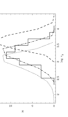
Figure 4: Comparison of the observed distribution of two-folding time-scales for 41 PG sample AGN (binsize $\Delta\log\tau_{\mathrm{2}}=0.2$, $N$ counts per bin) with the distributions predicted from random realisations of the broken power law power spectrum (with break frequency $\nu_{\mathrm{bk}}$) which probably describes the red-noise optical variability in AGN (10000 lightcurves simulated, $N$ rescaled to 41 counts over whole distribution).
Solid histogram: observed distribution, dotted line: $\nu_{\mathrm{bk}}=10^{-7}$ Hz, dot-dashed line: $\nu_{\rm bk}=2\times 10^{-8}$ Hz, dashed line: $\nu_{\mathrm{bk}}=4\times 10^{-9}$ Hz.

The lightcurves for this dataset (G99) show a typical intrinsic variability amplitude of $\sigma_{B}$ = 0.14 mag with intrinsic rms amplitudes of 5$\%<\sigma_{B}/B<$34$\%$ over the seven year period. The variability time-scales lie approximately between 300 and 4500 days. The distribution of two-folding time-scales is shown in Figs. 3 and 4 and the individual time-scales and luminosities for each AGN are given in Table 2. The mean two-folding time-scale for the sample is 1566.4 days and the corresponding standard deviation of the mean is 143.6 days (in log space, mean log $\tau_{\rm 2}=3.12\pm 0.04$).

Table 1: Individual minimum two-folding time-scales and luminosities for AGN in this PG subsample. The luminosity quoted is the median B band luminosity in the rest-frame of the source. Errors in the luminosities stem from errors in the observed magnitudes and hence the flux. Errors due to the uncertainty in $H_{0}$ are not included here.

Quasar	other names	z	RL	L${}_{4400\,\mbox{\AA}}\times$1042	$\tau_{\rm 2}$
				(erg s-1)	(days)
PG0026+129		0.142		11.9$\pm$0.22	1454
PG0052+251		0.155		20.7$\pm$0.38	318
PG0804+762		0.100		14.7$\pm$0.27	1009
PG0838+770		0.131		1.33$\pm$0.02	1907
PG0844+349	Ton 951	0.064		5.29$\pm$0.10	567
PG0923+201	Ton 1057	0.190		11.1$\pm$0.20	1158
PG0953+415	K 348-7	0.239		15.4$\pm$0.29	1266
PG1001+054		0.161		3.62$\pm$0.07	301
PG1012+008		0.185		16.6$\pm$0.31	1994
PG1048+342		0.167		1.29$\pm$0.02	496
PG1100+772	3C 249.1	0.313	Y	14.5$\pm$0.27	3186
PG1114+445		0.144		6.70$\pm$0.12	1901
PG1115+407		0.154		3.80$\pm$0.07	2262
PG1121+423		0.234		6.23$\pm$0.11	793
PG1151+117		0.176		6.64$\pm$0.12	608
PG1202+281	GQ Com	0.165		5.02$\pm$0.09	685
PG1211+143		0.085		13.5$\pm$0.25	1602
PG1229+204	Ton 1542	0.064		3.52$\pm$0.06	1189
PG1307+086		0.155		8.54$\pm$0.16	904
PG1309+355	Ton 1565	0.184	Y	10.4$\pm$0.19	1874
PG1322+659		0.168		6.10$\pm$0.11	4329
PG1351+640		0.087		9.92$\pm$0.18	1891
PG1354+213		0.300		3.69$\pm$0.07	1953
PG1402+261	Ton 182	0.164		8.47$\pm$0.16	2600
PG1404+226		0.098		2.16$\pm$0.04	1562
PG1411+442	PB 1732	0.089		7.35$\pm$0.14	2750
PG1415+451		0.114		2.90$\pm$0.54	1116
PG1426+015	Mkn 1383	0.086		4.08$\pm$0.07	1327
PG1427+480		0.221		3.95$\pm$0.07	1542
PG1444+407		0.267		2.80$\pm$0.05	3362
PG1512+370	4C 37.43	0.371	Y	10.7$\pm$0.20	3194
PG1519+226		0.137		3.38$\pm$0.06	1566
PG1545+210	3C 323.1	0.266	Y	10.3$\pm$0.19	1470
PG1613+658	Mkn 876	0.129		12.9$\pm$0.24	856
PG1617+175	Mkn 877	0.114		6.91$\pm$0.13	356
PG1626+554		0.133		5.91$\pm$0.11	668
PG1700+518		0.292		21.3$\pm$0.40	985
PG1704+608	3C 351	0.371	Y	22.5$\pm$0.41	954
PG2130+099	II Zw 136	0.061		7.50$\pm$0.14	1454
PG2233+134		0.325		11.8$\pm$0.22	2551
PG2251+113	PKS 2251+11	0.323	Y	17.00$\pm$0.31	2264

4.2 Distribution of two-folding time-scales

The optical variability of AGN is consistent with a red-noise process, so that each lightcurve is a realisation of an underlying process described by a power law power spectrum with a slope and amplitude determined by the mechanism which causes the variability. In principle, it is possible to derive the power-spectral parameters from the model for variability, and compare these with observations, however for simplicity and ease of interpretation we consider only the two-folding time-scale, which is a property of the power-spectral shape. Due to the stochastic nature of red-noise processes, lightcurves obtained at different times will look different, and show different observed two-folding time-scales. Ideally, we need to measure the ‘true’ average two-folding time-scale by averaging the two-folding time-scale over many 7-year lightcurves from the same source. As this is clearly not possible, we must take account of the fact that the two-folding time-scale measured for a given source is not the same as the average two-folding time-scale, and considerable scatter is introduced into the distribution of observed two-folding time-scales for sources which have identical variability properties (i.e. identical power-spectral shapes).
We can test whether the observed distribution of two-folding time-scales is consistent with a single power-spectral shape and amplitude (and a corresponding single average two-folding time-scale), by comparing the distribution we observe with that determined from simulated red-noise lightcurves generated from plausible power-spectral parameters. We therefore simulated random realisations of red-noise lightcurves using the method of Timmer & König (1995). To date, only the X-ray power-spectral shapes of AGN have been well constrained (Uttley, M^cHardy & Papadakis, 2002), showing fairly steep ($1/\nu^{2}$) power-law slopes at high frequencies, breaking to flatter $1/\nu$ slopes below some break frequency. The optical power-spectral shape of the AGN in our sample is not well constrained, but correlated long-time-scale optical/X-ray variations in the luminous Seyfert galaxy NGC 5548 suggest that although the optical power spectrum of luminous AGN is steeper than the X-ray power spectrum at high frequencies, the shapes are similar at low frequencies (Uttley et al. , 2003). Therefore we assume high-frequency power-spectral slopes of $1/\nu^{2.5}$, breaking to $1/\nu$ below some break frequency, $\nu_{\rm bk}$, which we assume is common to both X-ray and optical power spectra. Breaks in the X-ray power spectra of AGN appear to scale linearly with black hole mass (Uttley, M^cHardy & Papadakis, 2002), so we first chose a break frequency of $2\times 10^{-8}$ Hz, corresponding to a black hole mass of a few $\times~{}10^{8}$ M_⊙. We chose a power-spectral normalisation which corresponds to the typical observed $\sim 10$ per cent variability amplitude in the sample.
We simulated 10000 lightcurves of 7 year duration, and measured the resulting distribution of two-folding time-scale $\tau_{\rm 2}$, which is plotted for comparison with the observed distribution of $\tau_{\rm 2}$ in Fig. 4. We also show the distributions corresponding to break frequencies of $10^{-7}$ Hz and $4\times 10^{-9}$ Hz, i.e. a possible factor $\sim 25$ range in black hole mass. The observed distribution of $\tau_{\rm 2}$ is consistent with that expected from random realisations of a single power spectral shape expected from few $\times~{}10^{8}$ M_⊙ black holes. So the distribution of black hole masses is likely to be narrow ($<$ decade) and the variability in the lightcurves of all the AGN can be characterised by a single identical two-folding time-scale, as expected from a homogeneous sample of AGN such as that presented here. This result is not sensitive to the slope above the break. From Equation 6 the sample must also be consistent with a single value of the quantity $R_{\rm cut}^{3/2}/\alpha$. Keeping the Eddington ratio $L/L_{\rm Edd}$ fixed, there is a single value of the viscosity parameter $\alpha$ determined by the average $\tau_{\rm 2}$ of the sample.

For $0.01~{}\leq~{}L/L_{\rm Edd}~{}\leq~{}1.0$ the data are best fitted by the set of models outlined in Table 2.

Figure 5: This figure shows the allowed range of $\alpha$ values for both the blackbody models (left) and the modified blackbody models (right). The permitted values of $\alpha$ lie within the solid lines, the best fitting values lying along the dot-dashed line. The shaded areas are regions in which a given viscosity parameter, $\alpha$, and Eddington ratio, $L/L_{\rm Edd}$, cannot occur simultaneously in the model.

Fig. 5 shows the allowed values of $\alpha$ over a range of the Eddington ratio for both the disc models we apply. We note that the difference in viscosity between blackbody and modified blackbody models is small over this wavelength range.

Table 2: Model parameters for the PG data, with corresponding mass and accretion rate ranges of $10^{7}<M<10^{8.5}$ ( $\mbox{M}_{\odot}$) and $0.02<\dot{M}<0.70$ ( $\mbox{M}_{\odot}$ year^-1).

Model	$L/L_{\rm Edd}$	$\alpha_{\rm min}$	$\alpha_{\rm mean}$	$\alpha_{\rm max}$
disc blackbody	0.01	0.010	0.011	0.012
disc blackbody	0.1	0.015	0.017	0.018
disc blackbody	0.25	0.017	0.019	0.021
disc blackbody	0.5	0.020	0.022	0.025
disc blackbody	0.75	0.022	0.024	0.027
disc blackbody	1.0	0.023	0.026	0.028
modified blackbody	0.01	0.010	0.011	0.012
modified blackbody	0.1	0.015	0.017	0.018
modified blackbody	0.25	0.016	0.018	0.020
modified blackbody	0.5	0.019	0.021	0.023
modified blackbody	0.75	0.020	0.022	0.024
modified blackbody	1.0	0.021	0.023	0.026

5 Discussion

Since direct observations cannot yet resolve the inner accretion disc in AGN, numerical simulations of accretion flows have existed for several decades and are moving in the direction of global 3-D models. Our results fall within the range $0.005\leq\alpha\leq 0.6$ predicted by a variety of recent numerical simulations of MHD turbulent discs. However, we obtain much tighter constraints towards the lower end of this broad range which could eliminate some models. For example, Armitage (1998) writes that $\alpha\sim 0.1$ in global and local cylindrical disc simulations with net vertical field, whereas $\alpha\sim 0.01$ when the net vertical field is zero. MHD simulations have also shown that an alternative $\alpha$-prescription in which stress is proportional only to the magnetic pressure may be a better diagnostic of the viscosity mechanism, since using the Shakura Sunyaev (1973) $\alpha$-prescription a range of $\alpha$ values can be obtained for the same gas pressure (Hawley & Balbus, 1995).

The only previous observational viscosity estimates for AGN discs were those calculated by SC89 for 8 AGN and 4 blazars at 1060 Å , 3 AGN at 1395 Å  and 12 AGN at 1740 Å , with the prediction that $\alpha_{\rm min}=$ 0.001 and $\alpha_{\rm max}\sim$ 0.1. Our results allow a much tighter estimate of the viscosity range and we find a value around 0.02. Both estimates have used the same disc model, but at different wavelengths; we chose an optical sample rather than the UV data used by SC89 since the optical bands lie further from the peak in the power law region of the disc spectrum. SC89 assume an inclination angle of 0^∘ and include blazars in their sample. They discuss the likelihood that the interpretation of blazar variability as thermal changes in the accretion disc may not be valid since synchrotron radiation is known to dominate in many of these objects. They also note that the sampling of 5 of their sample objects was not designed for detecting the time-scales of interest when estimating disc viscosities. O’Brien et al.  (1988) examined IUE data of several AGN and found that most had UV two-folding time-scales of weeks to years with no shorter time-scale variability. The sampling rate for this data set was poor. Consequently, it would not be possible to estimate $\alpha$ for their sample. The PG subsample used here is larger and has a higher and more even sampling than any sample used in previous studies of this kind.

We find this sample of 41 AGN all have similar ($<$ decade) masses and therefore can all be represented by a single two-folding time-scale. Hence we find a very narrow range of $\alpha$ and/or $L/L_{\rm Edd}$. This seems to suggest that we are observing all these AGN in a single ’state’. If this is true, it may be that all observed AGN are in the outburst state and those in the quiescent state are either too faint to have yet been detected or appear as normal galaxies (Siemiginowska & Elvis 1997; Burderi, King & Szuszkiewicz 1998; Hatziminaoglou, Siemiginowska & Elvis 2001). If the former is true, this would then imply that the total number of AGN in existence is far higher than current estimates based on the number of sources we see. However, a single value of $\alpha$ throughout the thermal limit cycle has been predicted in some numerical simulations of MHD turbulence in AGN accretion disks (Menou & Quataert, 2001), though the thermal ionisation instability is unlikely to be a source of large amplitude variability in AGN.
Reverberation mapping measurements exist for 16 of these sources (Kaspi et al. , 2000) ranging from $2.16\times 10^{7}$ to $4.7\times 10^{8}\,\mbox{$\mbox{M}_{\odot}$}$ ($M_{\rm average}=1.51\times 10^{8}\,\mbox{$\mbox{M}_{\odot}$}$) with typical uncertainties of about 40 per cent. Black hole masses we find through the disc modelling method are dependent upon the ratio of AGN luminosity to the Eddington Limit, $L/L_{\rm Edd}$. For $L/L_{\rm Edd}=0.01$, $M=10^{8}-10^{8.5}\,\mbox{$\mbox{M}_{\odot}$}$ as suggested by comparing the observed distribution of two-folding time-scales with distributions predicted from random realisations of the broken power law power spectra. The reverberation mapping results are compatible with all the Eddington ratios used here.

We now summarise the main assumptions and note some caveats on our determination of $\alpha$. The accretion disc models we use are simple multi-temperature blackbody spectra (Czerny & Elvis 1987), and we assume that the disc is the source of the B Band luminosity. We also assume that long term variability in this band occurs on the thermal time-scale at a radius corresponding to a 50 per cent change in B Band luminosity. The limits on $\alpha$ are derived only for the sample as a whole since the variability time-scale and mass of each individual object is not precisely known. The results are dependent on the validity of the assumptions stated above and require a single viscosity value throughout the outer disc. In practice, viscosity is likely to be both radially and time dependent and variations in luminosity may occur on various time-scales and radii. For example, the $\alpha$ value we derive here would be a lower limit on the true value if the observed variability time-scales are not equal to but are longer than the thermal time-scale.

Blackbody and modified blackbody models gave very similar (and, at accretion rates one tenth of Eddington or lower, the same) values of $\alpha$. The small difference between the blackbody models and the addition of opacity effects to these models shows that in the optical B band, away from the peak of the emitted flux, electron scattering has only a small effect on the spectrum as expected.
The disc models do not include warps, clumpiness or flares. Contributions to the variability from occurrences of flares is, however, likely to be on time-scales shorter even than the sampling interval of the lightcurves.
G99 estimate pollution by the host galaxies to be approximately 5 per cent based on observations with HST (Bahcall et al. , 1997). The emission line contribution to the optical flux is estimated in the same paper at 5-10 per cent. The models applied here are for AGN continuum flux only and we have not reduced the observed flux to account for these since a 10 per cent luminosity increase will not greatly affect the viscosity estimates. We also note that our luminosity estimates are affected by the choice of $H_{0}$ which, if incorrect, would introduce an error into our results.
These models do not incorporate a corona, transition region, self-gravitation or irradiation of the disc material. Coronae are thought to be the source of hard X-rays but could alter the shape of the optical spectrum as we may see reprocessing and/or scattering, and this may be important in some AGN. The role of the corona in forming the continuum emission is discussed in Kurpiewski, Kuraszkiewicz & Czerny (1997) and a corona could be incorporated in future determinations of the $\alpha$-parameter.

There are currently no conclusive observational or theoretical bounds on the $\alpha$-parameter. We have carried out this study in the hope of providing another clue to the nature of viscosity in AGN.

6 conclusions

We assume that optical variability of AGN observed on time-scales of months to years is caused by local instabilities occurring on the thermal time-scale in the inner accretion disc. The disc is modelled using multi-temperature blackbody models. In this case we constrain the viscosity to

0.01 $\leq\alpha\leq$ 0.03 for $0.01\leq L/L_{\rm Edd}\leq 1.0$.

We show this sample is consistent with a single $\alpha$ value at a given Eddington ratio, determined by the average characteristic time-scale of all 41 AGN. The range of $\alpha$ values we find lies within the range predicted by current numerical simulations of MHD turbulent discs. The mass range we obtain for this sample is consistent with the reverberation mapping measurements made for 16 of these PG quasars. However, we do stress that this is a simplified model of an accretion disc, and merely a first step in observational viscosity estimates for AGN.

7 Acknowledgments

This work was partially supported by the NASA programs NAS8-39073 and Chandra Award Number GO1-2117B issued by the Chandra X-ray Observatory Center, which is operated by the Smithsonian Astrophysical Observatory for and on behalf of NASA under contract NAS8-39073. RLCS acknowledges support from a PPARC studentship. This research has made use of the NASA/IPAC Extragalactic Database (NED) which is operated by the Jet Propulsion Laboratory, California Institute of Technology, under contract with NASA.

References

- Armitage (1998) Armitage P. J., 1998, ApJ 501, L189
- Bahcall et al. (1997) Bahcall J. N., Kirhakos S., Saxe, D. H., Schneider, D. P., 1997, ApJ, 479, 642
- Balbus & Hawley (1991) Balbus S. A., Hawley J. F., 1991, ApJ, 376, 214
- Balbus & Hawley (1998) Balbus S. A., Hawley J. F., 1998, Revs. Mod. Phys. 70, 1
- Balbus & Papaloizou (1999) Balbus S., Papaloizou J., 1999, ApJ, 521, 650
- Berriman et al. (1990) Berriman G., Schmidt G. D., West S. C., Stockman H. S., 1990, ApJS, 74, 869
- Brandenburg et al. (1995) Brandenburg A., Nordlund Å., Stein R. F., Torkelsson U., 1995, ApJ 446, 874
- Burderi, King & Szuszkiewicz (1998) Burderi, L., King, A., Szuszkiewicz, E., 1998, ApJ, 509, 85
- Czerny & Elvis (1987) Czerny B., Elvis M., 1987, ApJ, 321, 305
- Accretion Power in Astrophysics (1992) Frank J., King A., Raine D., 1992, ‘Accretion Power in Astrophysics’, Cambridge University Press
- Giveon et al. (1999) Giveon U., Maoz D., Kaspi S., Netzer H., Smith P., 1999, MNRAS, 306, 637
- Haardt & Maraschi (1993) Haardt F., Maraschi L., 1993, ApJ, 413, 507
- Hatziminaoglou, Siemiginowska & Elvis (2001) Hatziminaoglou E., Siemiginowska A., Elvis M., 2001, ApJ, 547, 90
- Hawley & Balbus (1995) Hawley J. F., Balbus S. A., 1995, PASA 12, 159
- Hawley, Gammie & Balbus (1995) Hawley J. F., Gammie C. F., Balbus S. A., 1995, ApJ 440,742
- Kaspi et al. (2000) Kaspi S., Smith P. S., Netzer H., Maoz D., Jannuzi B. T., Giveon U., 2000, ApJ, 533, 631
- Kellermann et al. (1989) Kellermann K. I., Sramek R., Schmidt M., Shaffer D. B., Green R., 1989, ApJ, 98, 1195
- Kurpiewski, Kuraszkiewicz & Czerny (1997) Kurpiewski A., Kuraszkiewicz J., Czerny B., 1997, MNRAS, 285, 725
- Laor et al. (1997) Laor A., Fiore F., Elvis M., Wilkes B. J., McDowell J. C., 1997, ApJ, 477, 93
- Lightman & Eardley (1974) Lightman A. P, Eardley D. M., 1974, ApJ, 187, L1
- Malkan & Sargent (1982) Malkan M. A., Sargent W. L. W., 1982, ApJ, 254, 22
- Matsumoto & Shibata (1997) Matsumoto R., Shibata K., 1997, in ’Accretion Phenomena and Related Outflows’, Ed. Wickramsinghe D., Ferrario L. & Bicknell G., ASP San Francisco, 766
- Menou & Quataert (2001) Menou K., Quataert E., 2001, ApJ, 552, 204
- Neugebauer et al. (1987) Neugebauer G., Green R. F., Matthews K., Schmidt M., Soifer B. T., Bennett J., 1987, ApJS, 63, 615
- O’Brien, Gondhalekar & Wilson (1988) O’Brien P., Gondhalekar P., Wilson R., 1988, MNRAS, 233, 801
- Pica et al. (1988) Pica A. J., Smith A. G., Webb. J. R., Leacock R. J., Clements S., Gombola P. P., 1988, AJ, 96, 1215
- Schlegel et al. (1988) Schlegel D. J., Finkbeiner D. P., Davis M., 1988, ApJ, 500, 525
- Schmidt & Green (1983) Schmidt M., Green R., 1983, ApJ, 269, 352
- Shakura & Sunyaev (1973) Shakura N., Sunyaev R., 1973, A&A, 24, 337-355
- Siemiginowska & Czerny (1989) Siemiginowska A., Czerny B., 1989, MNRAS, 239, 289
- Siemiginowska & Elvis (1997) Siemiginowska A., Elvis M., 1997, ApJ, 482, L9
- Timmer & König (1995) Timmer J., König M., 1995, A&A, 300, 707
- Uttley et al. (2003) Uttley P. Edelson R., McHardy I. M., Peterson B. M., Markowitz A., 2003, ApJ, 584, L53
- Uttley, McHardy & Papadakis (2002) Uttley P., McHardy I. M., Papadakis I. E., 2002, MNRAS, 332, 231
- Webb & Malkan (2000) Webb W. & Malkan M., 2000, ApJ, 540, 652
- Weedman (1988) Weedman D. W., 1998, ‘Quasar astronomy’, Cambridge Astrophysics Series, Cambridge University Press