Parsec Scale Properties of Markarian 501

Abstract

We present the results of a high angular resolution study of the BL Lac object Markarian 501 in the radio band. We consider data taken at 14 different epochs, ranging between 1.6 GHz and 22 GHz in frequency, and including new Space VLBI observations obtained on 2001 March 5 and 6 at 1.6 and 5 GHz. We study the kinematics of the parsec-scale jet and estimate its bulk velocity and orientation with respect to the line of sight. Limb brightened structure in the jet is clearly visible in our data and we discuss its possible origin in terms of velocity gradients in the jet. Quasi-simultaneous multi-wavelength observations allow us to map the spectral index distribution and to compare it to the jet morphology. Finally, we estimate the physical parameters of the parsec-scale jet.

1 INTRODUCTION

BL Lac objects are one of the several flavors of radio loud active galactic nuclei. Along with peculiar properties at other wavelengths (lack of strong emission lines, high levels of variability, optical polarization up to 3%, detection at X-ray and $\gamma$-ray energies), they also show quite extreme behavior in the radio: the parsec-scale structure is dominated by a compact, flat-spectrum core, from which a one-sided jet emerges, showing knots of enhanced brightness. When monitored over long intervals, these components are often found to be in motion, sometimes with an apparently superluminal velocity (see, e.g., Homan et al., 2001).

The currently accepted explanation for these properties is found in the frame of unified models (see e.g. Urry & Padovani, 1995). These models are based on a dust enshrouded super-massive black hole accreting matter in a disk, from which two symmetric collimated jets of relativistic plasma are ejected in opposite directions. When the angle between the jet axis and the line of sight is small, the resulting Doppler boosting accounts for many of the above-mentioned properties.

A source such as Markarian 501 (B1652+39) is an ideal target to test the assumptions involved in unified models. At its low redshift ($z=0.034$), 1 mas = 0.72 pc; therefore, the milliarcsecond resolution achievable with VLBI techniques makes it possible to investigate in great detail the regions near the central core. Furthermore, Mkn 501 is one of the few sources with a clear limb-brightened structure (Giovannini, 1999; Aaron, 1999). Finally, this source is very well studied at other frequencies and it is known for its X$-$ and $\gamma-$ray (Quinn et al., 1996; Bradbury et al., 1997) activity, which also sets constraints on the parameters describing the physics of the inner jet (see Tavecchio et al., 2001; Katarzyński et al., 2001, and references therein).

In this paper we present a large multi-epoch, multi-frequency data-set of VLBI images; new observations as well as previously published data are used to study the physical properties of this source. In particular, we will discuss the pc-scale jet morphology, velocity and orientation. Additionally, our data-set allows us to compare images obtained at different frequencies with similar resolutions and thus to perform spectral index studies for comparison with the total intensity images.

In § 2 we describe the previous and new observations used in this paper, along with the data reduction methods and procedures for component fitting and spectral index mapping. Results are presented in § 3 and discussed in § 4. We present our conclusions in § 5.

2 OBSERVATIONS

Table 1 summarizes all observations considered in this paper, listing epoch, frequency, total observing time and array used. The notes provide references for details. The present data-set is very similar to the one used by Edwards & Piner (2002, hereafter EP02) to discuss the proper motion in Mkn 501: we did not use the 1995 Oct 17 epoch (due to its low sensitivity), or the 1996 Jul 10 and 1998 Oct 30 epochs (as better data from other nearby epochs was available). On the other hand, we add 3 more epochs (see note 4 to Table 1) at 15 and 22 GHz and we consider two new Space VLBI (VSOP) observations obtained on 2001 March 5 and 6 (see Table 2).

2.1 Data Reduction

2.1.1 Ground Observations

Images from some of the previous observations have been published or made available to the scientific community on open web sites. However, for the sake of completeness and homogeneity, we requested and obtained the calibrated ($u,v$)-data for all observations presented here. After the initial reduction (see notes to Table 1 for references), we imported the calibrated data into the NRAO Astronomical Image Processing System (AIPS) and inspected them carefully. Then, we produced new images; one or more self-calibration cycles proved to be useful in some cases, providing a better signal to noise ratio. We adopted the appropriate ($u,v$)-range, weights, cell-size and angular resolution to map the spectral index and to look for proper motion of the jet substructures; we present parameters of final images in Table 3.

2.1.2 Space VLBI Observations

We obtained Space VLBI images at three different epochs: 1997.8, 1998.4, and 2001.3. VSOP (VLBI Space Observatory Programme) observations combine data from ground arrays, such as the VLBA, and the 8 m orbiting antenna on board the satellite HALCA. For the latter two epochs observations at 1.6 and 4.8 GHz were performed on successive days to minimize flux density variability problems in spectral index mapping. The first Space VLBI observation was conducted at 1.6 GHz only. Further details on these observations are given in Table 2.

The standard VSOP observing mode has one polarization (LCP) and two IFs of 16 MHz each with two-bit sampled data. The lowest IF failed in the 1.6 GHz observation in 1997. In 2001, the “a priori” calibration was affected by lack of system temperature measurement for Robledo and Goldstone. A mini-cal procedure was done before starting the experiment in Robledo, providing a value of 20 K that was assumed as constant. For HALCA, we used the nominal system temperatures of 75 K and 77 K for the two IFs at 1.6 GHz, and 88 K and 92 K for those at 4.8 GHz (Hirabayashi et al., 1998, 2000).

All the data were correlated in Socorro and then imported and reduced in AIPS. Global fringe-fitting returned good solutions for all the observations in which large ground telescopes were used, although no solutions were found for the last observation (2001 Mar 6), unless a value of SNR as low as 4.5 was set in the fit. In spite of such a low signal to noise ratio, we found these solutions reasonable: delays and rates found in this way do not present any discontinuity or suspicious behavior. Thus, we applied these solutions and proceeded with the whole array.

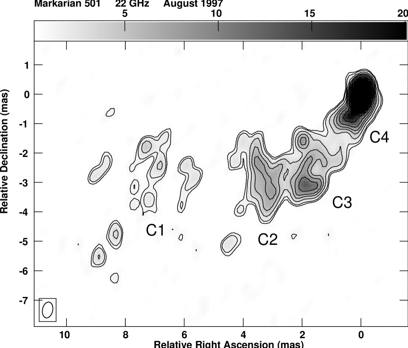
Figure 3: Isocontour level of Mkn 501 at 22 GHz from the August 1997 epoch. The HPBW is 0.54 $\times$ 0.35 mas in PA $-11^{\circ}$. The noise level is 0.3 mJy/beam. Contours are drawn at 1, 1.5 3, 5, 7, 10, 15, 20, 30, 50, 70, 100, 200, and 300 mJy/beam; the greyscale range is 0.3–20 mJy/beam. The limb brightened structure is visible even in the innermost region of the jet.

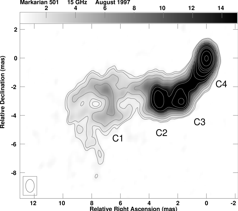
Figure 4: Isocontour level of Mkn 501 at 15 GHz from the August 1997 epoch. The HPBW is $0.6\times 0.9$ mas (RA $\times$ Dec). The noise level is 0.2 mJy/beam. Contours are drawn at 1, 1.5 3, 5, 10, 15, 20, 30, 50, 70, 100, 200, and 400 mJy/beam; the greyscale range is 0.3–15 mJy/beam. The limb brightening is clearly visible in the (resolved) C1 region, but no longer in the inner region because of the lower resolution.

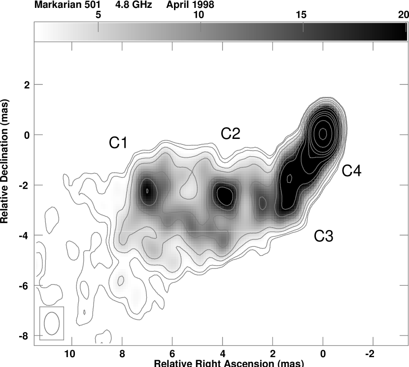
Figure 5: Gray scale plus isocontour level of Mkn 501 from the 5 GHz VSOP observation in April 1998. The HPBW is $0.6\times 0.9$ mas (RA $\times$ Dec). Contours are drawn at 1, 1.5 3, 5, 10, 15, 20, 30, 50, 70, 100, 200, and 400 mJy/beam; the greyscale range is 2–20 mJy/beam.

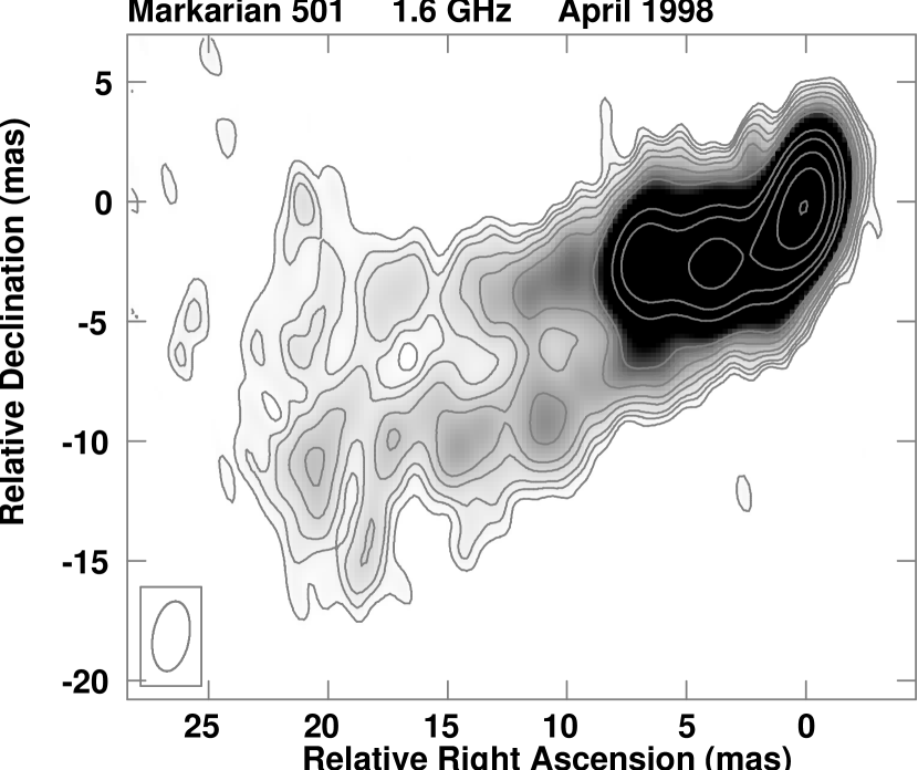
Figure 7: Gray scale plus isocontour level of Mkn 501 from the 1.6 GHz VSOP observation in April 1998. The HPBW is 3 $\times$ 1.5 mas at PA $-10^{\circ}$. Contours are drawn at 1, 1.5, 2, 3, 4, 6, 8, 10, 30, 50, 100, 200, and 400 mJy/beam; the greyscale range is 0.80–15 mJy/beam.

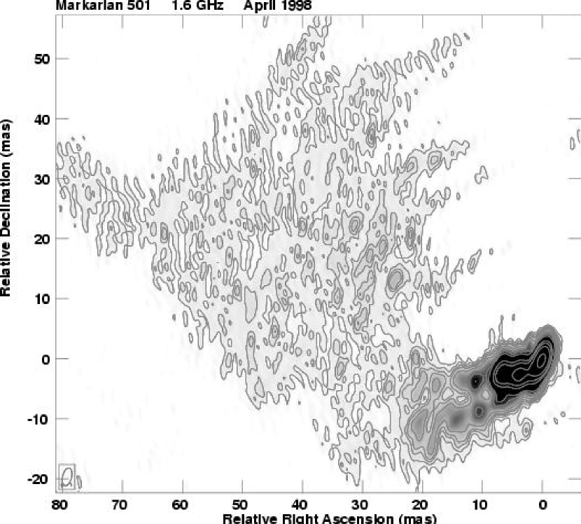
Figure 8: Gray scale plus isocontour level of Mkn 501 from the 1.6 GHz VSOP observation in April 1998. The HPBW is 3 $\times$ 1.5 mas at PA $-10^{\circ}$. Contours are drawn at 0.5, 1, 1.5, 2, 3, 5, 7, 10, 30, 50, 100, and 300 mJy/beam; the greyscale range is 0–10 mJy/beam.

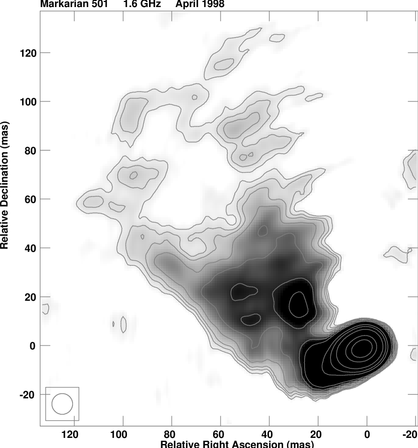
Figure 9: Gray scale plus isocontour level of Mkn 501 from the 1.6 GHz VSOP observation in April 1998. The image is convolved with circular beam of 8.5 mas FWHM. The image noise level is 0.4 mJy/beam. Contours are drawn at 1, 1.5, 2, 3, 5, 7, 10, 30, 50, 100, 300, and 500 mJy/beam; the greyscale range is 0.50–8 mJy/beam.

We then performed self calibration using clean-component models, first in phase and, afterward, in both phase and amplitude. In the latter, we repeated the task several times, increasing the baseline range. This revealed to be of great importance for those observations where gain information for some antennas was missing. For example, we could self-calibrate the shortest space-ground baselines using ‘uniform weight’ ground-only images; in fact, we have similar baselines both in the ground array and to HALCA, as provided by its highly elliptical orbit (see Fig. 1, 2). Figures 3 – 9 present all the images, in order of decreasing angular resolution.

2.2 Component Fitting

Identification of components is usually the most difficult problem affecting proper motion studies. Long time intervals between epochs can lead to misidentification of components; moreover, the use of different resolutions can cause confusion, for example by blending components with different properties and velocities; finally, registering images at different observing frequencies is also necessary: the apparent core shift due to the different spectral index of the core and jet can be significant.

In the present work, the time coverage is very dense (14 epochs over 4 years, plus the final VSOP observation) and there are no large time gaps. To prevent angular resolution problems, we produced maps at the same resolution at all epochs. Even if some observations allowed a better resolution, we convolved all the images obtained at a frequency 5 GHz $\leq\nu\leq$ 15 GHz with a circular restoring beam of 1.2 mas FWHM. However, higher resolution maps have also been made, in order to provide more information when needed. In particular we obtained images at a resolution of 0.6 $\times$ 0.9 mas (RA $\times$ Dec) in all observations with good $(u,v)$-coverage on long baselines (see Table 3). A comparison of fit components in convolved and full resolution images revealed good agreement.

The fit to the components of the jet was done within AIPS and the Difmap package. In AIPS we used the task JMFIT, which allows one to fit Gaussian components to part of an image. Up to four components can be used at a time and the task, starting from given initial conditions, solves in an iterative way for position, flux density and extension of each component. Since more than four components are needed to properly fit the images, we had to run the task several times on different regions. The regions were made to overlap with each other in order to obtain results compatible with previously published models. We also repeated the fit looking for “stable” solutions, i.e., changing our initial guesses or even leaving them blank. Eventually, very good models were obtained; the difference in flux density between our fits and the images is always smaller than 5%.

Using Difmap, we also carried out model-fitting to the visibilities rather than the image. Similarly to the fits made in AIPS, four to six jet components were required in addition to the core to provide a good representation of the data.

2.3 Spectral Index Mapping

When producing spectral index images, there are three main effects that have to be carefully taken into account. First, because of flux density variability and possible proper motion of components, the observations must be taken at very close epochs. Next, the angular resolution must be the same at both frequencies and the $(u,v)$-coverage as similar as possible; this guarantees the same sensitivity to extended structures in the high and low frequency images. Finally, as absolute position is not available, we need to properly align the images before combining them.

To meet the first two requirements, we produced spectral index images using data separated by less than 24 hrs. We considered 15 and 22 GHz data obtained on the same day (1997 Aug 15) and Space VLBI observations at 1.6 and 5 GHz made on successive days (1998 Apr 7 and 8 — see Edwards et al., 2000, for a preliminary analysis). We note that 1998 Space VLBI observations have better $(u,v)$-coverage than those in 2001 (see Fig. 1, 2). To obtain matching $(u,v)$-coverages, we cut the shortest baselines from the low frequency data and the longest baselines in the high frequency observations. Images were then obtained using uniform weights, and the same cell-size and restoring beam.

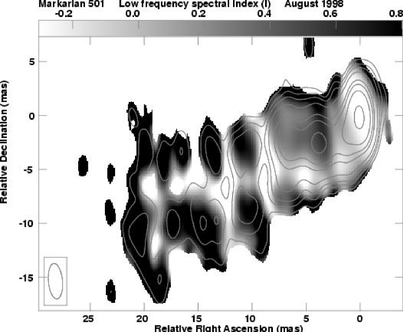
Figure 10: Low frequency, low resolution spectral index image: $\alpha_{1.6}^{4.8}$ with 3 $\times$ 1.5 mas HPBW (PA $10^{\circ}$). Contours show total intensity levels at 1.5, 3, 5, 10, 30, 50, 100, and 300 mJy/beam (at 1.6 GHz); the greyscale is the spectral index from $-0.3$ (inverted) to 0.8 (steep).

The problem in registering the images is that the peak of the image, coincident with the core, can correspond to different positions at different frequencies if the core is self-absorbed. So, we aligned the images using the positions of components along the jet in a region with steep spectral index and no self-absorption effects. We found that at 15 and 22 GHz no shift was necessary, while a shift of $\sim$0.2 mas was necessary in both RA and Dec between the 5 and 1.6 GHz images. See Figures 10 – 12 for the final spectral index maps.

3 RESULTS

3.1 Source Morphology

The large scale radio structure has been imaged with the VLA (Ulvestad et al., 1983; Van Breugel & Schilizzi, 1986; Cassaro et al., 1999), showing a core dominated source with two-sided diffuse emission oriented at $\mbox{PA}\sim 45^{\circ}$; this indicates that the jets are non relativistic at a (projected) distance of $\sim 10$ kpc from the core. The pc-scale structure has also been investigated, using VLBI techniques (see e.g. Conway & Wrobel, 1995), with resolution of $\sim 10$ mas. However, the collection of multi-epoch, multi-frequency, high resolution and high sensitivity images will improve our knowledge of the source morphology and evolution. The present VLBI observations show a strong core and a one-sided jet. The jet exhibits multiple sharp bends before undergoing a last turn, followed by rapid expansion. We can distinguish three different regions:

• a first region, extending $\sim 10$ mas from the core, where a high brightness jet structure is present (Fig. 3, 4, and 5). The jet PA is not constant in this region, being 150^∘ – 160^∘ near the core ($<$ 1 mas) and moving to $\sim 145^{\circ}$ (from 1 to $\sim$ 4 mas from the core) to become $\sim 90^{\circ}$ from 4 to 10 mas.

  The 22 GHz high resolution image (Fig. 3) shows that the jet is resolved and limb-brightened starting at $\sim$ 1 mas from the core. This is confirmed by the high sensitivity 5 GHz Space VLBI image (Fig. 5); although this image does not have enough angular resolution to resolve the inner jet near to the core, it shows an extended low brightness emission, confirming the transverse extension of the jet in the inner 2 mas. In the region from 2 to 10 mas from the core, the limb brightened jet structure is clearly visible.

  The brightness profile along the main axis of the jet is not uniform; high brightness regions are followed by dimmer regions. In particular at 5–6 mas from the core a deep minimum is present just before an extended bright spot with a peak 8–9 mas from the core. However, we do not refer to these regions as “knots”, since they are resolved at higher frequencies.

• between $\sim$ 10 mas and $\sim$ 30 mas from the core, the jet loses its collimation and becomes visible only in lower resolution images (Fig. 6, 7). In this region, the jet is oriented at a PA of $\sim$ 110^∘ and its opening angle is increasing. A well defined limb brightened structure is visible (see, e.g., Fig. 7), in agreement with the “layered” structure visible in the polarized emission (Aaron, 1999). As in the first region, lower frequency images reveal a wider jet and a more evident external shear layer; this implies that the spectra in the inner regions are flatter than in the external regions.

• at $\sim$ 30 mas from the core the jet shows strong bending and a large opening angle (Fig. 8, 9). In this third region the orientation of the diffuse jet is in agreement with the orientation of the kpc-scale emission. The jet opening angle is $\sim$ 43^∘. The radio brightness is uniform and there is no indication of the helical structure suggested by Conway & Wrobel (1995), which possibly resulted from the poor $(u,v)$-coverage (five telescopes only) of their observations. A limb-brightened structure is visible in our low resolution images up to $\sim$ 100 mas from the core, as can be seen in Fig. 9.

No radio emission is detected either on the opposite side of the radio core or in the position of the putative counterjet feature F reported by Conway & Wrobel (1995). However, if we compare our measured total flux densities to single dish data (e.g. from the UMRAO database), the correlated VLBI flux density accounts only for a part of the total flux density ($\sim 70$% at 5 GHz and $\sim 65$% at 15 GHz); this is in agreement with the presence of a larger scale structure resolved out by the VLBI data, such as the two sided emission shown by Ulvestad et al. (1983) and Cassaro et al. (1999).

3.2 Radio Flux Densities and Variability

Single dish monitoring of Markarian 501 shows that this source is remarkably stable in the radio band. Venturi et al. (2001) monitored a sample of 23 $\gamma-$ and X$-$ ray loud blazars over a 4 year period (1996–2000) with the 32 m Medicina radio telescope. From their data, Markarian 501 is the most quiescent source, with an almost flat light curve at both 5 and 8.4 GHz. Moreover, Markarian 501 is part of the UMRAO database, which also shows a fairly steady flux density. During the period of our observation, the average flux densities are $(1.54\pm 0.12)$ Jy at 4.8 GHz, $(1.53\pm 0.13)$ Jy at 8 GHz and $(1.29\pm 0.08)$ Jy at 14.5 GHz.

We consider the VLBI core flux density using our data at 15 GHz (0.6 $\times$ 0.9 mas FWHM, RA $\times$ Dec), where we have 8 different epochs (see Table 3). Assuming the map peak as the core flux density, we see some dispersion in the values, which range between 360 mJy (1997 Apr 25) and 508 mJy (1995 Dec 15). This suggests possible core variability, which is diluted in single dish observations, since the VLBI core makes up only $\sim 30$% of the total flux density. We note, however, that our observations are not homogeneous and were not aimed to monitor flux density variability.

3.3 Proper Motion

The overall morphology of the source does not present dramatic changes between epochs. No compact jet component (knot) is present in the jet at all frequencies: if we consider the highest resolution data, the local peaks present in the low resolution images become clearly resolved. Therefore, we limit our study to the innermost region, where high-resolution images are available (the jet brightness is too low to be detected at high frequency beyond 10 mas from the core). In this region, the jet is always transversally resolved: it appears centrally peaked at low resolution, but resolved with a limb brightened structure at high resolution. This implies that we could be mixing together different components with different properties and moving at different velocities. For all these reasons, we analysed images at the best angular resolution (typically 0.6 $\times$ 0.9 mas, RA $\times$ Dec) and, in model-fitting, we tried to use a number of components that did not produce an oversimplified representation of the data. In particular, to avoid resolution or frequency effects, we used only 15 GHz data, plus the 8.4 GHz observation at epoch 1998.48. The results obtained from model-fitting of visibilities in Difmap are presented in Table 4 and Fig. 13. These results are in agreement with those obtained by fitting Gaussian components to the images (using JMFIT in AIPS).

The data are in general well fitted by a core and four jet components, in agreement with EP02 (not surprisingly, as most data are the same). We labelled components according to the same notation for ease of comparison: C1 to C4 moving from the outermost component inward. However, for the reasons stated above, we adopted two Gaussians for each of the components C2 and C1 at many epochs. This produced a better fit to the data, in agreement with the resolved limb-brightened jet structure present in these regions. Nominal position errors are very small. The major uncertainty is related to the complex source structure. We estimate a position error of $\leq$0.1 mas for C4, C3, C2 and $\sim$ 0.2 mas for C1.

From our analysis we conclude that no proper motion is visible in any of the four components. Consider the case of component C2: EP02 measured a proper motion of $(0.6\pm 0.1)c$ for this component. However, we note that at the position of C2 two faint external peaks are visible in the 22 GHz image (Fig. 3) on either side of the lower frequency component. They could even have a different spectrum (Fig. 10). The peak position visible at lower resolution in the 15 GHz image is therefore the blend of the limb-brightened structure visible at 22 GHz. In the space VLBI image at 5 GHz, the component C2 is at a different position with respect to the 15 GHz images: this could be due to different spectra for the different components. We conclude that it is not possible to measure a proper motion for such a complex structure and that any pattern velocity measurement from low resolution data is not related to the jet bulk speed in this source.

3.4 Bulk Motion

Under the assumption of intrinsically symmetric two-sided jets affected by Doppler boosting effects, the observational data allow one to estimate the jet bulk velocity. In the following, we present the results derived from a study of the jet/counterjet ratio, core dominance and jet expansion.

3.4.1 Jet/Counterjet Ratio

From the lack of detection of a counter-jet in all the images (§ 3.1), we set a lower limit on the jet/counterjet ratio. We use the highest ratio between the jet brightness and the counterjet upper limit. We estimate this ratio excluding the innermost region of the jet; this avoids contamination from the unresolved central emission. The best image for this analysis is the Space VLBI observation obtained in Apr 1998 at 1.6 GHz. From this image we can derive a jet/counterjet ratio $R>1250$ (1 rms) at $\sim$ 4 mas from the core. Given the well known relation $R=\left(\frac{1+\beta\cos\theta}{1-\beta\cos\theta}\right)^{2+\alpha}$, and assuming $\alpha=0.5$ (see §3.5), this value yields $\beta\cos\theta>0.89$. In turn, this implies $\beta>$ 0.89 and $\theta<$ 27^∘.

Our deep, low resolution images allow us to also put a constraint at large distance from the core. In particular, in the 1.6 GHz image from the 2001.3 data, at $\sim 60$ mas from the core we still have R $>$ 70; although less extreme, this value is also very interesting, as it implies that the jet remains at least mildly relativistic ($\beta\cos\theta>0.69$) even at large distances from the core.

It is not possible to extend this analysis further with our data. However, we remind the reader of the symmetric morphology of the source on the kpc scale (§ 3.1). This implies that the bulk of the jet slows to subrelativistic speed going from the parsec to the kpc scales.

3.4.2 Core Dominance

Given the general relation between total and core radio power (Feretti et al., 1984; Giovannini et al., 1988, 2001; de Ruiter et al., 1990), we can use low frequency unboosted data to compute an “expected” value for the core power. A comparison between the expected and measured 5 GHz core radio power allows to constrain the jet orientation and velocity (Giovannini et al., 2001). We note that at 5 GHz self-absorption effects are small (see § 4.2); however, to take also into account possible core variability, we allow the observed core flux density to vary by a factor of 2. This is a conservative assumption, based on the total flux density monitoring and the range of derived VLBI core flux densities (see § 3.2), and, more generally, on statistical flux density variability of AGN in the radio.

To estimate the orientation and jet velocity for Mkn 501, we have compared its total unboosted flux density (1.81 Jy) at 408 MHz (Ficarra et al., 1985), with the nuclear flux density at 5 GHz. Since Giovannini et al. (2001) used the arcsecond core radio power to derive their correlation, we adopted the total VLBI correlated flux density at 5 GHz ($\sim$ 800 mJy) as the Mkn 501 core flux density. Any possible underestimate in this assumption is compensated for by the allowed range (a factor of 2) in flux density variability. We found that Mkn 501 has to be oriented at $\theta\leq$  27^∘ with $\beta\geq$ 0.88. We note that a high jet velocity ($\beta>$ 0.95) is allowed only in the range 10^∘ $<$ $\theta$ $<$ 27^∘. High velocities are forbidden at smaller angles; the resulting Doppler factor would require a core much brighter than observed.

3.4.3 Adiabatic Model

The functional dependence of the jet intensity on the jet velocity and radius for an adiabatically expanding jet has been discussed in the case of relativistic motion by Baum et al. (1997). Since the model represents a simplification of the real situation, the results should be considered with caution and compared with other observational results. This model has enabled useful constraints to be placed, in agreement with other data, for 3C 264 (Baum et al., 1997) and other sources, such as NGC 315 (Cotton et al., 1999) and 3C 449 (Feretti et al., 1999).

To apply this model we used our deep VSOP observations at 1.6 GHz obtained in March 2001 and in April 1998. In these observations, the jet emission is visible on scales up to $\sim 150$ mas (see, e.g., Fig. 9). First, we derived brightness profiles across the jet; we used the AIPS task SLICE on an image reconstructed with a circular beam of 7 mas diameter, where the longest baselines have been omitted to increase the signal to noise ratio. In the innermost region ($<25$ mas from the core), we have 8 slices, taken every half beam-width at PA 27.2^∘. After the main bend, we considered 12 more slices, each one beam apart, at PA $-57.1^{\circ}$. We stopped our analysis $\sim 100$ mas from the core; further out, the low jet brightness and the presence of extended sub-structures do not allow the data to be fitted well.

Using the AIPS task SLFIT, we fitted single Gaussians to each profile. This could be done unambiguously in most cases, although in a few slices some deviation from a pure single Gaussian profile was present. However, the difference between the area subtended by the profile and the fit is always smaller than 5% and does not affect the analysis. We plot the resulting FWHMs and peak brightnesses in Fig. 14 and 15; the quantities have been deconvolved from the CLEAN beam, according to the formula given by Killeen et al. (1986). There are clearly two regimes; least-squares fits yield a power-law of index $-3.2$ in the inner jet ($<30$ mas from the core) and $-1.3$ in the outer regions. In the following, we use these best-fit solutions rather then the actual data; this prevents us from spurious results brought about by random fluctuations.

We recall the equations given in Baum et al. (1997) for the jet surface brightness $I_{\nu}$:

$I_{\nu}\propto(\Gamma_{j}v_{j})^{-(\delta+2)/3)}r_{j}^{-(5\delta+4)/3)}D^{2+\alpha}$ (predominantly parallel magnetic field)

$I_{\nu}\propto(\Gamma_{j}v_{j})^{-(5\delta+7)/6)}r_{j}^{-(7\delta+5)/6)}D^{2+\alpha}$ (predominantly transverse magnetic field).

We assume an injection spectral index $\delta=2$, as suggested from the average $\alpha$ in the image, excluding the self-absorbed core (§ 3.5). It is not easy to decide which magnetic field regime is preferable: according to the 8.4 GHz images of Aaron (1999), the Mkn 501 jet is highly polarized at the edges with the magnetic field parallel to the jet flow, while in the jet spine the magnetic field is orthogonal to the jet flow with a lower degree of order. Pollack et al. (2003) report a 5 GHz electric vector PA distribution consistent with this result but the lower resolution renders the results less conclusive. Therefore, since the percentage of ordered field and the intrinsic orientation are not well known, we consider the two cases of pure parallel and perpendicular magnetic field orientation; in a disordered magnetic field, the real result will be in between the two extreme situations. Figure 16 shows the derived trends of $\beta$ for an initial Lorentz factor $\Gamma=3.2$ and $\Gamma=15$ ($\beta_{i}=0.95,0.998$) with parallel and perpendicular magnetic fields. In each plot, we draw five lines, corresponding to angles to the line of sight of 5^∘, 10^∘, …, 25^∘ (i.e., in the range of values allowed by the jet sidedness and core dominance).

We note that the jet velocity decreases with the core distance, more slowly in the perpendicular case, and on a shorter scale in the parallel case. The lack of detection of the CJ in all our images strongly constrains any possible model since it implies a relativistic jet also at large distance from the core ($>50$ pc). Models with low initial Lorentz factor ($\Gamma<5$) are definitely ruled out, regardless of the assumed magnetic field orientation, since they disagree with both the observed limb-brightened structure (§ 4.1.1) and the jet/counterjet ratio (at least in the case of the parallel magnetic field); moreover, they require a jet deceleration (§ 4.1.1) between the $\gamma-$ray region and radio jet region that is too strong. Among models with a higher initial speed ($\Gamma=15$), the case of the parallel magnetic field requires an orientation angle of 25^∘, at least at $>$ 70 mas from the core, to be in agreement with the observed jet/counterjet brightness ratio. We cannot exclude models with a narrow angle to the line of sight at small distances from the core, where solutions are similar. In the case of the perpendicular magnetic field, the constraints are less severe since we have a fast jet even at large distances from the core.

3.5 Spectral Index

In Fig. 10, 11 and 12, we display the spectral index distribution at various resolutions between 1.6 and 4.8 GHz and between 15 and 22 GHz. Observational results are summarized in Table 5 for high resolution images and described in the following subsections.

3.5.1 Low Frequency Range: $\alpha^{1.6}_{4.8}$

At low resolution ($3.3\,\times\,1.3$ mas, PA = $5^{\circ}$), we can study the spectral index distribution at distances from the core larger than 8–10 mas (Fig. 10). The limb-brightened jet structure between 8 and 20 mas from the core is clearly visible. The spectrum is always flat in the inner spine (medium value $\alpha$ = 0.08) and steep in the bright shear regions, with values in the range $0.9\sim 2.1$. In the inner region ($<$ 8 mas from the core), the jet is well resolved with a steep spectrum in the more external regions ($0.7\sim 1.0$) but with a puzzling region south of the high brightness region where the spectral index is $\alpha\sim-0.1$. This region is clearly visible also in the lower resolution image in Edwards et al. (2000) where it seems connected to the inner spine flat spectrum region, while no such connection is present in the total intensity images.

Using the space VLBI baselines, we can study the source details at higher angular resolution ($1.7\times 0.9$ mas, PA = $-25^{\circ}$) even at this frequency (Fig. 11). The nuclear spectrum is inverted ($\alpha^{1.6}_{4.8}=-0.45$). Except for C4 (confused with the core and subject to a large uncertainty), the jet sub-components show flat to moderately steep spectra: $0.1<\alpha^{1.6}_{4.8}<0.6$. Regions in between the components have steeper spectra.

3.5.2 High Frequency Range: $\alpha^{15}_{22}$

At these high frequencies, we are beyond the self-absorption turnover and the nuclear region shows a flat, non-inverted spectrum ($\alpha$ = 0.45), generally steepening along the jet. The resolution of 0.6 $\times$ 0.9 mas (RA $\times$ Dec, Fig. 12) shows that the inner regions C4, C3, C2 have $\alpha^{15}_{22}$ in the range $0.60\sim 0.80$, while regions in between are much steeper ($\alpha\sim 2$ and higher). The large component C1 is too faint and resolved to be properly imaged at these high frequencies. A marginal suggestion is present of a spectral steepening moving from the inner (spine) to the external jet region but at this high angular resolution the jet width is not well defined.

3.5.3 Average Nuclear Spectrum

It is interesting to consider the nuclear flux density over the whole range of frequency. We are aware that the compact core of Mkn 501 presents some variability (see §3.2); however, the large number of observations and frequencies available allow us to carry out such a study based on average values.

We plot in Fig. 17 the average core peak flux density, from the images at resolution of 0.6 $\times$ 0.9 mas (see Table 3); at 1.6 GHz, we had to consider super-resolved images, in order to avoid a large contamination from the jet. The spectrum is convex, peaking at $\sim 8.4$ GHz and steepening toward the high frequency end. Below the turnover frequency, the spectrum is flatter than $\alpha=2.5$, as would be expected for a single self-absorbed component. This suggests that different components with different turnover frequencies may be blended together.

4 DISCUSSION

4.1 Jet Velocity

4.1.1 Velocity Structure

Limb brightened jet morphology on parsec scales is present in some FR I sources but also in a few high power FR II sources (Giovannini et al., 2002). A possible explanation is the presence of velocity structure in the jet. When viewed at a relatively large angle to the line of sight, this structure yields different Doppler factors for the internal spine and the external shear layer. In particular, an inner high velocity spine could be de-boosted while a slower external layer could be less strongly de-boosted, or even boosted. Transverse jet velocity structure has been found by Laing et al. (1999, 2002a, 2002b) in 3C 31, where the jet velocity in outer regions is $\sim$ 0.7 the inner spine velocity. Chiaberge et al. (2000) invoke such a structure to account for observational discrepancies between FR I and BL-Lac objects.

A possible origin of the velocity structure is the interaction of the jet with the surrounding medium and its consequent entrainment; the mass loading slows down the jet in the external regions, while the inner spine travels unaffected. However, the presence of limb brightened jets in both high and low power sources (Giovannini et al., 2002) and the evidence in M87 that the jet structure is present very near to the core emission (see the image presented by Junor et al., 1999), suggest the possibility that the velocity structure may originate at the base of the jet. Meier (2003) presents a model where the inner high velocity spine is produced in the black hole region, while the external shear moving at lower velocity is produced in a more extended region downstream.

In Mkn 501, it is interesting to note that the jet structure is visible at a distance $<$ 1 mas from the core, suggesting that it originates very close to the base of the jet. However, we recall that, at $z=0.034$, 1 mas corresponds to $\sim 0.7$ pc, i.e., $>10^{4}$ Schwarzschild radii (see Rieger & Mannheim, 2003, and references therein for a discussion on the central black hole mass in Mkn 501) and, therefore, we do not have the angular resolution to see this jet inner region. Nevertheless, we note that the presence of velocity structure so near to the nuclear source implies too strong a deceleration if it is completely due to the jet interaction with the ISM. We suggest (in agreement with M87 data of Junor et al., 1999) that a transverse velocity gradient is intrinsic to the jet structure (as discussed by Meier, 2003) and that a further velocity decrease due to mass loading in the jet from the ISM is likely to be present and possibly dominates the jet velocity structure at larger distances from the core.

4.1.2 Bulk Motion and Jet Orientation

We have strong indications that in Mkn 501 the radio jet emission is oriented at a large angle with respect to the line of sight relative to that expected for a blazar:

• From the jet morphology: the jet is limb-brightened in high resolution images at $\sim 1$ mas from the core. The different brightness can be related to a different Doppler factor only with an orientation angle $\theta$ $>$ $\sim$15^∘. Then, we can reproduce the observed ratio between the brightness of the external shear and the inner spine with $\Gamma_{spine}=15$, assuming $\Gamma_{layer}\sim 3$ (see Tables 6, 7). With these values, the spine Doppler factor ($\delta_{spine}$) is lower than the external layer Doppler factor ($\delta_{layer}$). On the contrary, a jet orientation at a smaller angle and/or a lower spine velocity imply $\delta_{spine}>\delta_{layer}$ and therefore a centrally peaked structure.

• From the core dominance: the core boosting is high but not extreme; high bulk velocities require, therefore, an orientation angle $\theta$ in the range 10^∘–27^∘ with respect to the line of sight.

• From the fit to the trend of the jet brightness and FWHM: assuming an adiabatic model and consistency with the jet/counterjet brightness ratio, we need a radio jet starting with a high velocity ($\beta\sim$ 0.998), and in the case of a parallel magnetic field, $\theta$ has to be $\sim$ 25^∘ at $>$ 70 mas.

These results seem to be in disagreement with constraints derived from the high frequency ($\gamma$-ray) emission and variability detected in blazars. Studying the rapid burst of TeV photons in Mkn 421, Salvati et al. (1998) determine that a jet with a bulk velocity $\Gamma$ $>$ $\sim$ 10 with opening angle and orientation angle $\sim 1/\Gamma$ is required. Similarly, in Mkn 501 the expected Doppler factor should be $>$ $\sim$ 10, as obtained from fits of synchrotron self-Compton (SSC) models (Katarzyński et al., 2001; Tavecchio et al., 2001). To reconcile the radio and high frequency results we have to assume that the inner region of the jet (0.001–0.03 pc) is moving with a Lorentz factor $>$ $\sim$ 10 and oriented at $\theta\,\raise 2.0pt\hbox{$<$}\kern-11.00008pt\lower 4.0pt\hbox{$\sim$}\ 5^{\circ}$. From this region we have high energy radiation and negligible radio emission. Over the range from 0.03 to 50 pc (projected distance) the jet orientation has to change from $\sim$ 5^∘ to 25^∘ (or at least $\sim 15^{\circ}$ in the case of perpendicular magnetic field).

We propose that this large change in the jet direction may be gradual and we derive the minimum change requested by observational data at different distances from the core. As shown in Table 6, a progressive change in the jet direction with respect to the line of sight is possible and in agreement with the observed pc-scale jet properties.

At present, there is no obvious explanation for this change in the jet direction in the inner region. It is possible that it could be related to helical type motion (Villata et al., 1999) (although helical motion is not visible in our high resolution images), or to an instability in the jet due to reasons that are thus far unknown. It is also important to stress that small changes in direction are not uncommon in FR I radio galaxies and are magnified when projection effects occur. In any case, we recall that beyond 30 mas from the core the jet position angle becomes stable and closely aligned with the kpc-scale structure.

We note that in the case of the perpendicular magnetic field the jet velocity is still very high at large distances from the core, in agreement with the lack of detection of a visible counterjet in all published maps of this source and despite the symmetric structure visible in the VLA low resolution image (Ulvestad et al., 1983). However, we recall that $\theta\ \raise 2.0pt\hbox{$>$}\kern-11.00008pt\lower 4.0pt\hbox{$\sim$}\ 15^{\circ}$ is required to justify the observed limb-brightened structure from Doppler boosting alone, even in the case of perpendicular magnetic field.

4.2 Physical Parameters

From the present data we can derive that:

• The nuclear region shows a self-absorbed spectrum with a peak frequency $\nu_{m}\sim 8.4$ GHz and a peak flux density $S_{m}\sim 0.55$ Jy. Following Marscher (1987), we can use these data to estimate the magnetic field in the nuclear region (from 0.03 to 0.15 pc):

  B = $3.2\times 10^{-5}\,\theta^{4}\,\nu^{5}_{m}\,S^{-2}_{m}\,\delta\,(1+z)^{-1};$

  assuming $\theta$ (the core angular size) = 0.2 mas (0.15 pc) and $\delta$ = 5 (Table 6), we estimate a magnetic field B $\sim$ 0.03 gauss. On the other hand, fits of SSC models to a high energy state observed in April 1997 yield values of the magnetic field in the range 0.2–0.02 gauss in the inner region ($<$ 0.03 pc) (Katarzyński et al., 2001). This suggests a constant or a not very large decrease of the magnetic field from the gamma ray emitting region to the beginning of the radio jet.

• The radio spectra of jet sub-components show an evident steepening at high frequencies, suggesting the effect of radiative losses in a high magnetic field.

• In the region where the jet is well resolved, the spectrum is flat in the inner spine confirming the presence of a higher transport efficiency, lower radiative losses, or reacceleration mechanisms. The transverse steepening from the spine to the shear layer regions confirms the larger losses in these regions, probably related to the interaction with the external medium.

• It is not straightforward to determine the equipartition magnetic field (Pacholczyk, 1970) given the complex structure of the jet. We can obtain a rough estimate by assuming that electrons and heavy particles carry the same amount of energy ($K=1$), the filling factor $\phi$ = 1, and the frequency range is between 10 MHz and 100 GHz. This yields $\sim$ 0.015 gauss in the C4 and C3 regions and 0.01 gauss in the C2 and C1 regions.

• Assuming a viewing angle $\theta$ as in Tables 6 and 7, the observed angular distances correspond to the following de-projected linear distances:

  – The inner limb-brightened region is present at $<$ 4 pc from the core

  – The first jet region extends to $\sim$ 10 mas, corresponding to $\sim$ 30 pc

  – The VLBI jet is visible up to 170–270 pc (assuming $\theta$ = 25^∘ – 15^∘, respectively)

  – The kpc-scale structure is symmetric (i.e. not relativistic) at $\leq 20-30$ kpc from the core

  – The large scale symmetric structure extending to $\sim$ 70^′′ corresponds to a linear size of 120–200 kpc, in agreement with the expected linear size of a FR I radio galaxy with the same low frequency total radio power.

5 CONCLUSIONS

As a result of the many frequencies and resolutions available, we have established that a limb-brightened structure is indeed present in Markarian 501, beginning in the very inner jet. This has important consequences: (1) it implies the presence of velocity structure already at very small scale, which jet models will have to take into account; (2) it suggests, together with other arguments, that the VLBI jet can not be oriented at too small a viewing angle. In particular, the detection of a very long one-sided jet and the results of an adiabatic expansion fit yield values of the angle of view in the range $15^{\circ}<\theta<25^{\circ}$, depending also on the magnetic field orientation.

The bulk velocity is strongly relativistic at the beginning ($\Gamma\sim 15$), decreasing to $\beta\sim 0.6$ ($\Gamma\sim$ 1.25) at the end of the VLBI jet, 100 mas from the core (parallel $B$) or to $\beta\sim 0.99$ ($\Gamma\sim 7$) in the case of a perpendicular $B$. The data considered here are consistent with a pattern speed of zero. Previous reports, based mostly on lower frequency observations, have reported low pattern speeds, however the complex limb-brightened structure revealed at 22 GHz makes measurement of component speeds problematic at high frequencies.

Finally, the study of the spectral indices has revealed a self-absorbed compact core and a complex spectral index distribution in the jet with flat and very steep regions. A clear connection is present between limb-brightening in total intensity and the spectral index images: the inner spine has a flat spectrum while the jet more external regions show steep spectra. Our derived magnetic field strengths are similar to those obtained from data at other wavelengths, yielding values of order $B\sim 0.03$ gauss in the core region. The estimated equipartition field in the jet region is in the range 0.015–0.01 gauss.

Table 1: Observation List

Date	Frequency	Array	Observing Time
	(GHz)		(min)
1995 Apr 7	15	VLBA	40
1995 Apr 12	8.3	VLBA	15
1995 Dec 15	15	VLBA	40
1996 Apr 23	8.3	VLBA	7.5
1996 Apr 23	15	VLBA	6
1996 Jun 7	8.1	VLBA	6
1997 Mar 13	15	VLBA	40
1997 Apr 25	15	VLBA	90
1997 Apr 25	22	VLBA	90
1997 May 26	15	VLBA	50
1997 May 26	22	VLBA	50
1997 Aug 4	1.6	VLBA$-$SC+GO+HALCA	420
1997 Aug 15	15	VLBA	40
1997 Aug 15	22	VLBA	40
1998 Apr 7	4.8	VLBA+EB+HALCA	780
1998 Apr 8	1.6	VLBA+RO+GO+HALCA	600
1998 Jun 24	8.4	VLBA+GC+GN+KK+	20
		MC+ON+WF
1999 Jul 19	15	VLBA$-$SC	40
2001 Mar 5	1.6	VLBA+GO+RO+HALCA	480
2001 Mar 6	4.8	VLBA$-$HN+HALCA	540

Note. — EB, Effelsberg (Germany) 100 m, GC, Gilcreek (USA) 26 m GN, Green Bank (USA) 20 m; GO, Goldstone (USA) DSN 70 m; HN, Hancock VLBA 25 m; KK, Kokee Park (USA) 20 m; MC, Medicina (Italy) 32 m; ON, Onsala (Sweden) 20 m; RO, Robledo (Spain) DSN 70 m; SC, St. Croix VLBA 25 m; WF, Westford (USA) 18 m.

Table 2: Summary of VLBA+HALCA Observations

Date	Frequency	Obs. Time	Tracking	Other
	(GHz)	(hr)	Stations	Telescopes
1997 Aug 4	1.6	7	NZ ($3^{h}$)	GO ($4^{h}$)
1998 Apr 7	4.8	13	RZ ($2.7^{h}$+$1.1^{h}$), NZ ($3.3^{h}$)	EB
1998 Apr 8	1.6	10	RZ ($3.6^{h}$), NZ ($4^{h}$)	GO, RO
2001 Mar 5	1.6	8	RZ ($1^{h}$), NZ ($2^{h}$)	RO ($4^{h}$), GO ($7.5^{h}$)
2001 Mar 6	4.8	9	RZ ($0.5^{h}$), NZ ($1^{h}$)	$\cdots$

Note. — RZ, Robledo tracking station; NZ, Green Bank tracking station; EB, Effelsberg (100 m); RO, Robledo (70 m); GO, Goldstone (70 m).

Table 3: Observational Parameters

Date	Frequency	HPBW	Noise Level	Peak Flux Density
	(GHz)	(mas)	(mJy/beam)	(mJy/beam)
1995 Apr 7	15	0.6 $\times$ 0.9	0.20	485
		1.2	0.25	524
1995 Apr 12	8.3	1.2	0.40	524
1995 Dec 15	15	0.6 $\times$ 0.9	0.35	508
		1.2	0.30	546
1996 Apr 23	8.3	1.2	0.25	521
	15	0.6 $\times$ 0.9	0.30	490
		1.2	0.35	520
1996 Jun 7	8.1	1.2	0.40	535
1997 Mar 13	15	0.6 $\times$ 0.9	0.15	381
		1.2	0.20	410
1997 Apr 25	15	0.6 $\times$ 0.9	0.10	360
		1.2	0.15	390
	22	0.3 $\times$ 0.5	0.15	327
1997 May 26	15	0.6 $\times$ 0.9	0.10	408
		1.2	0.10	438
	22	0.4 $\times$ 0.6	0.20	334
1997 Aug 4	1.6	1.5 $\times$ 2.9	2.3	409
1997 Aug 15	15	0.6 $\times$ 0.9	0.20	455
		1.2	0.15	487
	22	0.3 $\times$ 0.5	0.25	350
1998 Apr 7	4.8	0.6 $\times$ 0.9	0.40	465
		1.2	0.25	509
1998 Apr 8	1.6	1.5 $\times$ 2.9	0.12	421
1998 Jun 24	8.6	0.6 $\times$ 0.9	0.25	477
		1.2	0.35	508
1999 Jul 19	15	0.6 $\times$ 0.9	0.20	446
		1.2	0.20	480
2001 Mar 5	1.6	1.5 $\times$ 2.9	0.50	316
2001 Mar 6	4.8	1.2	0.50	428

Table 4: Results of the Model - Fitting

Epoch	Component	Distance from core
		(mas)
1995.29	C4	0.6
	C3	2.4
	C2	4.3
	C1	7.6
1995.96	C4	0.7
	C3	2.6
	C2	4.0
	C1a	7.4
	C1b	7.5
1996.29	C4	0.5
	C3	2.6
	C2	4.0
	C1a	7.7
	C1b	7.8
1997.21	C4	0.6
	C3	2.6
	C2a	3.7
	C2b	3.9
	C1a	7.7
	C1b	7.9
1997.29	C4	0.6
	C3	2.3
	C2a	3.7
	C2b	4.0
	C1	7.8
1997.37	C4	0.6
	C3	2.5
	C2a	3.8
	C2b	4.1
	C1a	7.7
	C1b	7.9
1997.62	C4	0.7
	C3	2.4
	C2a	3.6
	C2b	4.4
	C1a	7.3
	C1b	8.0
1998.48	C4	0.8
	C3	2.7
	C2	4.7
	C1	7.4
1999.55	C4	0.7
	C3	2.6
	C2	4.5
	C1a	7.8
	C1b	8.9

Table 5: Spectral Index Results

Image	beam	PA	core	C4	C4toC3	C3	C3toC2	C2	C2toC1	C1
$\alpha^{1.6}_{4.8}$	$1.7\times 0.9$	$-25^{\circ}$	$-0.45$	$-0.2^{*}$	$0.6^{*}$	0.1	0.9	0.6	0.7	0.3
$\alpha^{15}_{22}$	$0.6\times 0.9$	$0^{\circ}$	0.45	0.80	2	0.65	$\cdots$	0.70	2.4	resolved

Note. — Results of the spectral index imaged in Figures 11, 12. Typical uncertainties are $\pm 0.05$. Data marked with an asterisk (*) are estimated after core subtraction and have larger uncertainties.

Table 6: Jet Velocity Structure - Parallel Magnetic Field

Rcore	$\theta$	$\Gamma_{spine}$	$\delta_{spine}$	$\Gamma_{layer}$	$\delta_{layer}$	Notes
(pc)	(∘)
0.0001 – $<$0.03	4	15	15	?	?	$\gamma$-ray region
0.03 – 0.15	10	15	4	10	5	Radio core
0.15 – 7	15	15	2	3	5	First jet region
7 – 20	15–20	15	2–1	3	4–3	Before of large bending
20–30	25	10–3	1–2	2	2.5	After the large bending
50	25	1.25	1.8	1.1	1.5	Final VLBI jet region

Note. — R_core = projected distance from the core

Table 7: Jet Velocity Structure - Perpendicular Magnetic Field

Rcore	$\theta$	$\Gamma_{spine}$	$\delta_{spine}$	$\Gamma_{layer}$	$\delta_{layer}$	Notes
(pc)	(∘)
0.0001 – $<$0.03	4	15	15	?	?	$\gamma$-ray region
0.03 – 0.15	10	15	4	10	5	Radio core
0.15 – 7	15	15	2	3	5	First jet region
7 – 20	15	15	2	3	4	Before of large bending
20–30	15	10	2.5	3	4	After the large bending
50	15	10	2.5	3	4	Final VLBI jet region

Note. — R_core = projected distance from the core

Figure 1: ($u,v$)-coverage of the Space VLBI observation at 1.6 GHz ($\lambda=18$ cm) on 1998 April 8. Available separately as .jpg file figure01.jpg

Figure 2: ($u,v$)-coverage of the Space VLBI observation at 4.8 GHz ($\lambda=6$ cm) on 1998 April 7. Available separately as .jpg file figure02.jpg

Figure 6: Isocontour level of Mkn 501 from the 5 GHz VSOP observation in April 1998. The HPBW is 2 $\times$ 1 mas in PA $-20^{\circ}$. Contours are drawn at $-$3, 1.5, 2, 3, 5, 10, 20, 30, 40, 50, 100, 300, and 500 mJy/beam.

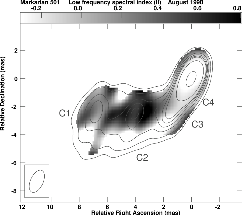
Figure 11: Low frequency, high resolution spectral index image: $\alpha_{1.6}^{4.8}$ with 2 $\times$ 1 mas HPBW (PA $-20^{\circ}$). Contours show total intensity levels at 5, 10, 20, 30, 40, 50, 100, 400 mJy/beam (at 4.8 GHz); the greyscale is the spectral index from $-0.3$ (inverted) to 0.8 (steep).

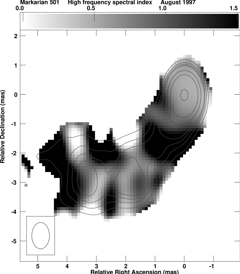
Figure 12: High frequency, high resolution spectral index image: $\alpha_{15}^{22}$ with $0.6\times 0.9$ mas HPBW (RA $\times$ Dec). Contours show total intensity levels at 5, 10, 15, 20, 50, 100, and 400 mJy/beam (at 15 GHz); the greyscale is the spectral index from 0 (flat) to 1.5 (steep), where $S(\nu)\propto\nu^{-\alpha}$.

Figure 13: Component positions from model-fitting. Distances are given in milliarcsecond. All points are at 15 GHz, with the exception of the 1998.48 epoch which is at 8.4 GHz.

Figure 14: Plots of peak brightness (top) and FWHM (bottom) of Gaussian model fits vs. distance from the core. Straight lines represent least-squares fits. There is a clear change in behavior at about 35 mas from the core.

Figure 15: Plots of peak brightness vs. FWHM of Gaussian model fits. Straight lines represent least-squares fits. The change in behavior visible in Fig. 14 corresponds to the change in slope at FWHM $\sim 15$ mas. The power law slopes are $-3.2$ and $-1.3$.

Figure 16: Results of the adiabatic model fit. The low initial velocity with parallel magnetic field is at top; middle and bottom plots show high initial velocities ($\beta_{i}=0.998$) for a parallel and perpendicular magnetic field, respectively. Orientation angles of $5^{\circ},10^{\circ},15^{\circ},20^{\circ},25^{\circ}$ are drawn in each plot, with angle increasing from bottom left to top right. For illustration purposes, the vertical axis in the bottom plot spans only the range 0.8–1.

Figure 17: Average core spectrum from data at resolution 0.6 $\times$ 0.9 (HPBW, RA $\times$ Dec). Note the turnover at 8.4 GHz and the rapid decrease at higher frequency. The low frequency part presents a slow growth, suggesting the presence of more than one single self-absorbed component.

References

- Aaron (1999) Aaron, S. 1999, ASP Conf. Ser. 159: BL Lac Phenomenon, 427
- Baum et al. (1997) Baum, S. A. et al. 1997, ApJ, 483, 178
- Bradbury et al. (1997) Bradbury, S. M. et al. 1997, A&A, 320, L5
- Cassaro et al. (1999) Cassaro, P., Stanghellini, C., Bondi, M., Dallacasa, D., della Ceca, R., & Zappalà, R. A. 1999, A&AS, 139, 601
- Chiaberge et al. (2000) Chiaberge, M., Celotti, A., Capetti, A., & Ghisellini, G. 2000, A&A, 358, 104
- Conway & Wrobel (1995) Conway, J. E. & Wrobel, J. M. 1995, ApJ, 439, 98
- de Ruiter et al. (1990) de Ruiter, H. R., Parma, P., Fanti, C., & Fanti, R. 1990, A&A, 227, 351
- Cotton et al. (1999) Cotton, W. D., Feretti, L., Giovannini, G., Lara, L., & Venturi, T. 1999, ApJ, 519, 108
- Edwards et al. (2000) Edwards, P. G., Giovannini, G., Cotton, W. D., Feretti, L., Fujisawa, K., Hirabayashi, H., Lara, L., & Venturi, T. 2000, PASJ, 52, 1015
- EP02 (2002) Edwards, P. G. & Piner, B. G. 2002, ApJ, 579, L67
- Feretti et al. (1984) Feretti, L., Giovannini, G., Gregorini, L., Parma, P., & Zamorani, G. 1984, A&A, 139, 55
- Feretti et al. (1999) Feretti, L., Perley, R., Giovannini, G., & Andernach, H. 1999, A&A, 341, 29
- Fey & Charlot (1997) Fey, A. L. & Charlot, P. 1997, ApJS, 111, 95
- Ficarra et al. (1985) Ficarra, A., Grueff, G., & Tomassetti, G. 1985, A&AS, 59, 255
- Giovannini et al. (1988) Giovannini, G., Feretti, L., Gregorini, L., & Parma, P. 1988, A&A, 199, 73
- Giovannini (1999) Giovannini, G. 1999 in BL Lac Phenomenon, ASP Conf. Ser., 159, 439
- Giovannini et al. (2000) Giovannini, G., Cotton, W. D., Feretti, L., Lara, L., & Venturi, T. 2000, AdSpR, 26, 693
- Giovannini et al. (2001) Giovannini, G., Cotton, W.D., Feretti, L. et al. 2001, ApJ, 552, 508
- Giovannini et al. (2002) Giovannini, G. 2002, NewAR in press (astro-ph/0302176)
- Hirabayashi et al. (2000) Hirabayashi, H. et al. 2000, PASJ, 52, 955
- Hirabayashi et al. (1998) Hirabayashi, H. et al. 1998, Science, 281, 1825 and erratum 282, 1995
- Homan et al. (2001) Homan, D. C., Ojha, R., Wardle, J. F. C., Roberts, D. H., Aller, M. F., Aller, H. D., & Hughes, P. A. 2001, ApJ, 549, 840
- Junor et al. (1999) Junor, W., Biretta, J. A., & Livio, M. 1999, Nature, 401, 891
- Katarzyński et al. (2001) Katarzyński, K., Sol, H., & Kus, A. 2001, A&A, 367, 809
- Kellermann et al. (1998) Kellermann, K. I., Vermeulen, R. C., Zensus, J. A., & Cohen, M. H. 1998, AJ, 115, 1295
- Killeen et al. (1986) Killeen, N. E. B., Bicknell, G. V., & Carter, D. 1986, ApJ, 309, 45
- Laing et al. (1999) Laing, R. A., Parma, P., de Ruiter, H. R., & Fanti, R. 1999, MNRAS, 306, 513
- Laing et al. (2002a) Laing, R. A. & Bridle, A. H. 2002a, MNRAS, 336, 328
- Laing et al. (2002b) Laing, R. A. & Bridle, A. H. 2002b, MNRAS, 336, 1161
- Ma et al. (1998) Ma, C. et al. 1998, AJ, 116, 516
- Marscher (1987) Marscher, A. P. 1987, Superluminal Radio Sources, 280
- Marscher (1999) Marscher, A. P. 1999, APh, 11, 19
- Meier (2003) Meier, D.L. 2002, NewAR in press
- Pacholczyk (1970) Pacholczyk, A. G. 1970, Radio Astrophysics (San Francisco: Freeman & Co.)
- Pollack et al. (2003) Pollack, L. K., Taylor, G. B., & Zavala, R. T. 2003, ApJ, 589, 733
- Quinn et al. (1996) Quinn, J. et al. 1996, ApJ, 456, L83
- Rieger & Mannheim (2003) Rieger, F. M. & Mannheim, K. 2003, A&A, 397, 121
- Salvati et al. (1998) Salvati, M., Spada, M., & Pacini, F. 1998, ApJ, 495, L19
- Tavecchio et al. (2001) Tavecchio, F., Maraschi, L., Pian, E. et al. 2001, ApJ, 554, 725
- Ulvestad et al. (1983) Ulvestad, J. S., Johnston, K. J. & Weiler, K. W. 1983, ApJ, 266, 18
- Urry & Padovani (1995) Urry, C. M. & Padovani, P. 1995, PASP, 107, 803
- Van Breugel & Schilizzi (1986) Van Breugel, W. & Schilizzi R. 1986, ApJ, 301, 834
- Venturi et al. (2001) Venturi, T. et al. 2001, A&A, 379, 755
- Villata et al. (1999) Villata, M. & Raiteri, C. M. 1999, A&A, 347, 30