The CMB Quadrupole in a Polarized Light

Abstract

The low quadrupole of the cosmic microwave background (CMB), measured by COBE and confirmed by WMAP, has generated much discussion recently. We point out that the well-known correlation between temperature and polarization anisotropies of the CMB further constrains the low multipole anisotropy data. This correlation originates from the fact that the low-multipole polarization signal is sourced by the CMB quadrupole as seen by free electrons during the relatively recent cosmic history. Consequently, the large-angle temperature anisotropy data make restrictive predictions for the large-angle polarization anisotropy, which depend primarily on the optical depth for electron scattering after cosmological recombination, $\tau$. We show that if current cosmological models for the generation of large angle anisotropy are correct and the COBE/WMAP data are not significantly contaminated by non-CMB signals, then the observed ${\cal C}_{\ell}^{TE}$ amplitude on the largest scales is discrepant at the $\sim 99.8\%$ level with the observed ${\cal C}_{\ell}^{TT}$ for the concordance $\Lambda$CDM model with $\tau=0.10$. Using $\tau=0.17$, the preferred WMAP model-independent value, the discrepancy is at the level of 98.5%.

1. Introduction

The low quadrupole (and first few multipoles) of the cosmic microwave background (CMB), measured by COBE (Bennett et al. , 1996) and confirmed by WMAP (Bennett et al. , 2003), has generated much discussion recently, with several papers offering various possible causes for suppressed power on very large scales (e.g., Bond 1995, Efstathiou 2003a, Bridle et al. 2003, Contaldi et al. 2003, Tegmark et al. 2003, Cline et al. 2003, Feng & Zhang 2003, among others). Often in the case of measurements suggestive of new physics, the obvious way to advance is to perform a better experiment. However, the current measurements of the temperature anisotropy power spectrum of the CMB on large angular scales are already limited only by how well the Galaxy can be removed (Bennett et al. , 2003), and so the prospects for improved measurements are poor. In this work we point out that polarization measurements on large angular scales can test whether the temperature anisotropy on these scales is indeed generated within the standard cosmological framework.

The correlation between temperature and polarization anisotropies is well-known (Zaldarriaga & Seljak, 1997). It has been detected by Leitch et al. (2002) on intermediate angular scales and measured by the WMAP experiment on the scales of interest here (Kogut et al. , 2003). This correlation has been used to predict the polarization pattern on the sky from the observed temperature pattern (Jaffe, 2003). The correlation between temperature and polarization arises because the source of the polarization is Thomson scattering of the quadrupole anisotropy in the temperature of the radiation field. Spatial fluctuations in the monopole and dipole of the temperature field at the time of recombination seed higher multipole anisotropies by free-streaming (for a recent review see Hu & Dodelson 2002). Most of the large scale polarized signal we consider here originated from Thomson scattering of the CMB quadrupole at the relatively recent epoch following the reionization of the Universe (Zaldarriaga, 1997). The quadrupole temperature anisotropy seen by free electrons at this epoch receives a significant contribution to its $k$-space kernel from density fluctuation modes on scales $k^{-1}$ that also contribute to the present-day quadrupole (Tegmark & Zaldarriaga, 2002).

For a given realization of the CMB sky, the measured temperature anisotropy power at a given multipole, ${\cal C}_{\ell}^{TT}$ will have some amount of intrinsic scatter, as will the polarization anisotropy power, ${\cal C}_{\ell}^{EE}$ and the cross power spectrum, ${\cal C}_{\ell}^{TE}$ . Importantly, these measures of the power are correlated. If ${\cal C}_{\ell}^{TT}$ is measured to be low, then one would expect a low measure of ${\cal C}_{\ell}^{TE}$ and also a low value of ${\cal C}_{\ell}^{EE}$ . Therefore, if measures of ${\cal C}_{\ell}^{TE}$ and ${\cal C}_{\ell}^{EE}$ at low multipoles (large angular scales) are not “anomalously” low, then this would exacerbate the current tension with theoretical models (Spergel et al. , 2003).

$\Lambda$CDM is currently the standard cosmological model, and so we choose to assume the best-fit WMAP cosmological parameters and study how likely it is, from a frequentist perspective, that the observed data are simply realizations of this model. If the assumed model is in fact correct, then the correlations between observables provide statistical consistency checks. For example, flukes of cosmic variance should be partly correlated between temperature and polarization observables, so it might be expected that large outliers in the temperature data will have counterparts in the polarization data. Here, we present results of consistency tests using current data, and estimate the range of possible future data that could be comfortably accommodated within the currently accepted cosmological models.

2. TT–TE correlations

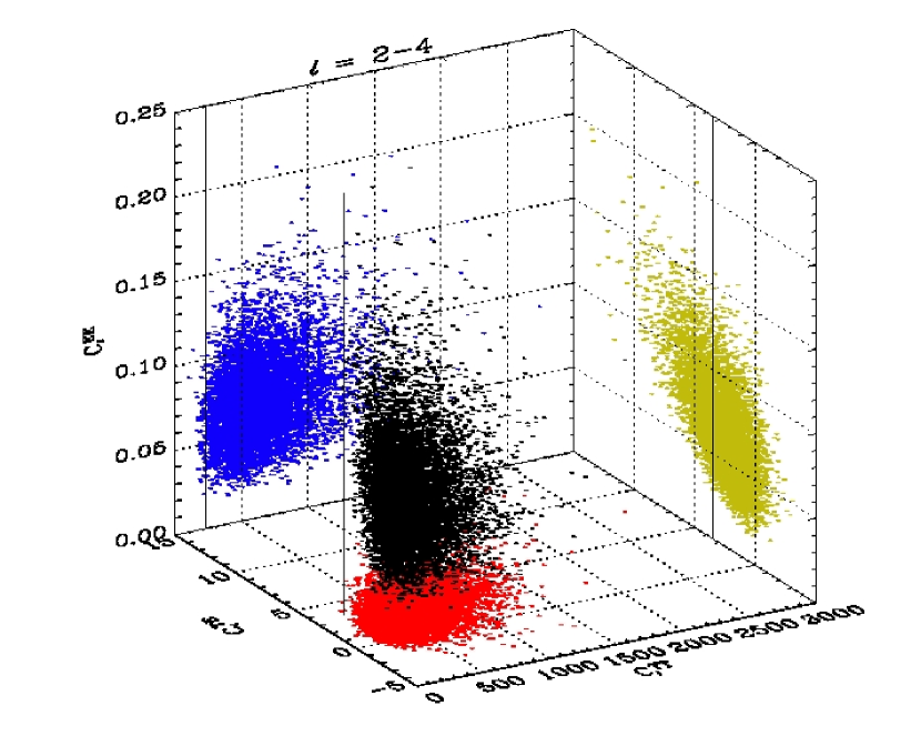
Figure 1.— 3D view (black points) of realizations of WMAP best fit model for $\ell=2-4$, assuming a noise model comparable to one year of WMAP observations. Projections are shown on the sides of the “box.” Center dark vertical line shows measured WMAP point in this space; there is no ${\cal C}_{\ell}^{EE}$ data released at this time so no constraint along the vertical axis. The horizontal ( ${\cal C}_{\ell}^{TE}$ , ${\cal C}_{\ell}^{TT}$ ) plane corresponds to Figure 3 whereas the vertical left ( ${\cal C}_{\ell}^{EE}$ , ${\cal C}_{\ell}^{TT}$ ) plane corresponds to Figure 4.

The correlations between the temperature and polarization power spectra can be used as a powerful consistency test. For example, it is possible to use the measured ${\cal C}_{\ell}^{TE}$ to construct a probability distribution for ${\cal C}_{\ell}^{TT}$ and compare this to measured values of ${\cal C}_{\ell}^{TT}$ . Alternatively, the measured ${\cal C}_{\ell}^{TT}$ can be used to estimate the most likely values of measured ${\cal C}_{\ell}^{TE}$ or to forecast future ${\cal C}_{\ell}^{TE}$ or ${\cal C}_{\ell}^{EE}$ measurements. We present examples of both these calculations below.

Explicit expressions for the covariance between power spectra, assuming Gaussian uncorrelated noise and Gaussian beams, are given by Zaldarriaga, Spergel, & Seljak (1997) and are useful for understanding the nature of the covariances. In all that follows we neglect beam effects since we are interested in very large scales, where $\ell$ is much smaller than the inverse of the beam size (in radians). All ${\cal C}_{\ell}^{X}$ (where $X$ corresponds to $TT$,$TE$, or $EE$) are in units of $\mu{\rm K}^{2}$.

3. Monte Carlo Methodology

We generate $10^{5}$ realizations of the WMAP-only best-fit cosmological model $a_{{\ell}m}$ ($\Omega_{m}h^{2}=0.13$, $\Omega_{b}h^{2}=0.023$, $h=0.68$, $n_{s}=0.97$, $A=0.8$ and $\tau=0.10$ as in table 1 of Spergel et al.  (2003)) and for $\ell<40$ we construct theoretical joint distributions of ${\cal C}_{\ell}^{EE}$ , ${\cal C}_{\ell}^{TE}$ and ${\cal C}_{\ell}^{TT}$ for this model. The scatter in these quantities around the input model is both due to cosmic variance and noise, and the scatter between different power spectra is somewhat correlated. We use the 1 year WMAP data for ${\cal C}_{\ell}^{TT}$ and ${\cal C}_{\ell}^{TE}$ from the corresponding publicly–available ASCII files .

We use a simple noise model which is as close as possible to that reported by the WMAP experiment after one year of operation. Specifically we assume that the white noise level corresponds to the use of 16 W-Band, 8 V-band and 8 Q-band channels (see table 1 in Bennett et al.  (2003)) with an effective sky fraction of $0.86/1.14$ (Verde et al. , 2003), so that we get $w_{T}^{-1/2}=1.07\times 10^{-1}\mu$K per (0.21)² sq. deg. pixel with a corresponding $w_{E}=w_{T}/2$. We add this white noise directly to the generated $a_{{\ell}m}$. This simple simulation scheme neglects the weak extra power at low ${\ell}$ originating from the residual $1/f$ noise (Hinshaw et al. , 2003). We neglect any non-gaussian systematic uncertainty that may be caused by improper subtraction of the galactic component (Bennett et al. , 2003; Efstathiou, 2003b). However, to assess the significance of our assumed level of noise, we also consider simulations where the noise amplitude, $w_{T}^{-1/2}$, was arbitrarily scaled up by a factor of $\sqrt{2}$, so that the noise contribution to the ${\cal C}_{\ell}^{X}$ errors is doubled. This excess noise could be either some unknown component of low frequency noise or residual galactic contamination (although the latter should probably not be modeled as a white noise).

Furthermore, to reduce the effects of covariance due to the real cut sky we consider bins of width $\Delta\ell=2$–$4$, where ${\cal C}_{\ell}^{X}$s are assumed constant. With such binned power spectrum estimates, the covariance between neighboring bins should be very small and our Monte Carlo results should approximate reasonably well the actual covariance of the properly measured ${\cal C}_{\ell}^{X}$ (we estimate that the correlation between our lower bins is less than 10%). It is important to note that our procedure is only approximate and it is therefore not strictly appropriate to compare our results directly to WMAP data; however we do not expect that more accurate simulations would alter significantly our conclusions.

4. Monte Carlo Results

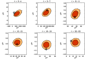
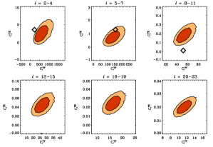
Figure 2.— Realizations of ${\cal C}_{\ell}^{TE}$ and ${\cal C}_{\ell}^{TT}$ for noise levels typical of one year of WMAP observations (2 upper rows) and for cosmic variance only (2 lower rows). WMAP data points are marked and the measurement noise and cosmic variance are included in the realizations (i.e. , it is appropriate for the points to not have error bars). The data points in the 2 lower rows are shown only for reference (as they contain noise).

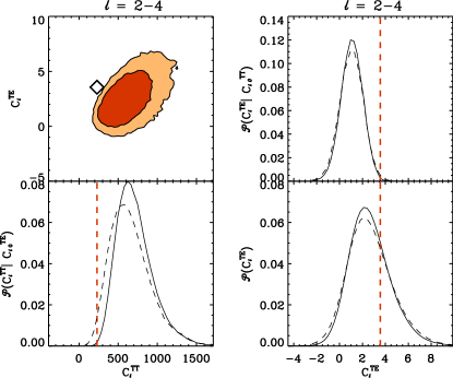
Figure 3.— Lowest multipole bin distribution of ${\cal C}_{\ell}^{TE}$ and ${\cal C}_{\ell}^{TT}$ assuming the WMAP best fit cosmological model and one year of observation (top left). The bottom right panel shows the likelihood distribution of ${\cal C}_{\ell}^{TE}$ with no information on ${\cal C}_{\ell}^{TT}$ , and the top right panel shows the likelihood subject to the constraint that ${\cal C}_{\ell}^{TT}$ has the measured value. The bottom left panel shows the likelihood of the ${\cal C}_{\ell}^{TT}$ given the observed ${\cal C}_{\ell}^{TE}$ . Dashed vertical lines indicate the measured WMAP values. The dashed distributions correspond to simulations where the noise level has been arbitrarily increased by a factor $\sqrt{2}$.

The result of these realizations is an ensemble of points in ( ${\cal C}_{\ell}^{TT}$ , ${\cal C}_{\ell}^{TE}$ , ${\cal C}_{\ell}^{EE}$ ) space, shown in Figure 1. Slices through this volume then provide a frequentist estimate of the expected joint distribution of spectra for this particular model. In particular, slices passing through observed points allow investigation of the conditional likelihoods in the other directions. For example, the vertical line shows the observed WMAP data and a histogram of points along this line would give the conditional probability of ${\cal C}_{\ell}^{EE}$ given the observed ${\cal C}_{\ell}^{TE}$ and ${\cal C}_{\ell}^{TT}$ .

In Figure 2 we show the distribution of expected ${\cal C}_{\ell}^{TT}$ and ${\cal C}_{\ell}^{TE}$ that would be observed, including our approximate WMAP noise model. Current data already provide a consistency check, even with the relatively large noise contribution to ${\cal C}_{\ell}^{TE}$ . On the largest angular scales the measurements are approaching the cosmic-variance limit for bins of size $\Delta\ell=3$, even with only one year of WMAP data. However, on slightly smaller angular scales the data contain a significant noise component, as can be seen in Figure 8 of Kogut et al.  (2003). This noise will be uncorrelated between the ${\cal C}_{\ell}^{TE}$ and ${\cal C}_{\ell}^{TT}$ power spectra and leads to the bins with $\ell\gtrsim 8$ showing little correlation in Figure 2.

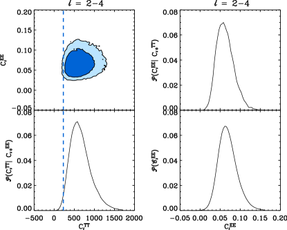
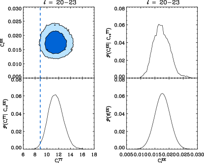
Figure 4.— Same as Figure 3, now for ${\cal C}_{\ell}^{EE}$ - ${\cal C}_{\ell}^{TT}$ covariance, again assuming a noise model comparable to one year of WMAP data. Here we show the multipole bins $2\leq\ell\leq 4$ (left) and $20\leq\ell\leq 23$ (right), the two largest outliers in the ${\cal C}_{\ell}^{TT}$ bins considered.

In Figure 2 we also show the ${\cal C}_{\ell}^{TT}$ - ${\cal C}_{\ell}^{TE}$ correlation for perfect measurements (no noise). The current low-$\ell$ ${\cal C}_{\ell}^{TT}$ data are significantly discrepant with the best-fit model, but equally remarkable is that the ${\cal C}_{\ell}^{TE}$ measurements on the largest scales are not particularly low. The measured ${\cal C}_{\ell}^{TE}$ on these scales is close to the middle of the expected range if one ignores the correlation with the ${\cal C}_{\ell}^{TT}$ data on these scales. However, the probability of the measured ${\cal C}_{\ell}^{TE}$ given the observed ${\cal C}_{\ell}^{TT}$ is extremely low if this is indeed a realization of the best fit model. The observed ${\cal C}_{\ell}^{TE}$ is in fact anomalous by not being low. This can be seen comparing the bottom right and top right panels of Figure 3. In the bottom right panel it can be seen that the observed ${\cal C}_{\ell}^{TE}$ on this scale is just in the range predicted by the best-fit model (26% of the models lie above the observed value). In the top right panel we see that this agreement disappears when we apply the condition that the observed ${\cal C}_{\ell}^{TT}$ is low (0.17% of the models lie above the observed value (or 0.85% when the $C_{\ell}^{X}$ noise is scaled up arbitrarily by a factor of 2). In realizations of the best-fit model it is rare that ${\cal C}_{\ell}^{TT}$ is as low as the value measured by WMAP, but in the few realizations where ${\cal C}_{\ell}^{TT}$ was low it was usually the case that the ${\cal C}_{\ell}^{TE}$ was also low. Correspondingly, middle-of-the-road ${\cal C}_{\ell}^{TE}$ values are unlikely to appear with low ${\cal C}_{\ell}^{TT}$ , as shown in the lower left panel. Specifically, 99.9% of the ${\cal C}_{\ell}^{TT}$ values are greater than the measured one given the measured value of ${\cal C}_{\ell}^{TE}$ , while when the measured ${\cal C}_{\ell}^{TE}$ is not included the fraction drops to 99.0% (with the corresponding numbers being 99.8% and 99.1% when the $C_{\ell}^{X}$ noise is arbitrarily doubled). These results are dictated by the profile of the joint ( ${\cal C}_{\ell}^{TT}$ , ${\cal C}_{\ell}^{TE}$ ) distribution in the top left panel of Figure 3.

Upcoming measurements of the ${\cal C}_{\ell}^{EE}$ power spectrum on large scales could shed some light on this problem. At the noise levels expected in the near future there is little correlation between the ${\cal C}_{\ell}^{EE}$ and ${\cal C}_{\ell}^{TT}$ power spectra, as shown in Figure 4, where the histograms in the right top and bottom panels are nearly unaffected when the temperature information is included. The 3D plot in Figure 1 again shows that the observed ${\cal C}_{\ell}^{TE}$ - ${\cal C}_{\ell}^{TT}$ large angle pair (shown as a vertical line) is exceedingly unlikely, but also shows that there is a fairly tight correlation between ${\cal C}_{\ell}^{TE}$ and ${\cal C}_{\ell}^{EE}$ on these scales. This provides an important consistency check on our understanding of the CMB. The observed ${\cal C}_{\ell}^{TE}$ - ${\cal C}_{\ell}^{TT}$ pair on these scales reduces significantly the expected range of ${\cal C}_{\ell}^{EE}$ (assuming the best fit model).

5. Cosmological Implications

The correlations between power spectra have several cosmological implications.

Figure 5.— Probability for ${\cal C}_{\ell}^{TE}$ larger than the observed value, given the observed ${\cal C}_{\ell}^{TT}$ value for $2<l<4$, ${\cal P}({\cal C}_{\ell}^{TE}>{\cal C}_{{\ell}0}^{TE}|{\cal C}_{{\ell}0}^{TT})$, as a function of the optical depth value $\tau$ (solid line). Also shown, for reference, is the same probability without the condition on the observed ${\cal C}_{\ell}^{TT}$ value (dashed line). All cosmological parameters are kept the same as in our fiducial $\Lambda$CDM model except for $\tau$ and $n_{s}$ that are changed simultaneously along the $\tau$–$n_{s}$ degeneracy line favored by WMAP. The power-spectrum amplitude is marginalized over. Note that ${\cal P}({\cal C}_{\ell}^{TE}>{\cal C}_{{\ell}0}^{TE}|{\cal C}_{{\ell}0}^{TT})$ does not exceed 5$\%$.

So far we assumed the best-fit WMAP value for the optical depth to electron scattering after cosmological recombination, $\tau=0.10$ (Spergel et al. , 2003; Kogut et al. , 2003) and a power-law primordial power spectrum.

Adopting a different optical depth $\tau$ has a significant but still limited effect on our results. We repeated the analysis by considering various optical depth values and the results are shown in Figure 5. The solid line shows the probability for 2$\leq{\ell}\leq$4 of having ${\cal C}_{\ell}^{TE}$ larger than the observed value given the observed ${\cal C}_{\ell}^{TT}$ value, ${\cal P}({\cal C}_{\ell}^{TE}>{\cal C}_{{\ell}0}^{TE}|{\cal C}_{{\ell}0}^{TT})$, and the dashed line shows the same without the condition on the observed ${\cal C}_{\ell}^{TT}$ value, ${\cal P}({\cal C}_{\ell}^{TE}>{\cal C}_{{\ell}0}^{TE})$. All cosmological parameters were held fixed except for $\tau$ and $n_{s}$ which were varied in the ranges 0.05–0.29 and 0.95–1.05 respectively, along the $n_{s}-\tau$ degeneracy line favored by WMAP [see Figure 5 of Spergel et al. (2003)]. The power spectrum amplitude $A_{s}$ was marginalized over. Other parameters will have little impact on the large-angle polarization, as shown in Kaplinghat et al.  (2003). A complete frequentist treatment, allowing all parameters to vary from their best fit, is unlikely to lead to qualitatively different results.

Increasing $\tau$ makes the observed ${\cal C}_{\ell}^{TE}$ more likely, but is not sufficient to alleviate the tension between the low ${\cal C}_{\ell}^{TT}$ and the average ${\cal C}_{\ell}^{TE}$ : note that ${\cal P}({\cal C}_{\ell}^{TE}>{\cal C}_{{\ell}0}^{TE}|{\cal C}_{{\ell}0}^{TT})$ does not exceed 5%. Note that this tension is not included in current estimates of the optical depth. In previous analyses of WMAP data, the ${\cal C}_{\ell}^{TT}$ likelihood is multiplied by the bottom right panels rather than the top right panels of Figure 3. For all but the largest angular scales (the first few multipoles) this effect is negligible, but it is clear from Figure 5 that the direction of the bias is such that the current estimates of $\tau$ are likely to be low.

Additional suppression of the matter power spectrum on large scales tends to reduce the discrepancy of the current ${\cal C}_{\ell}^{TT}$ data, but not by a large amount. The mapping from matter power spectrum to temperature anisotropies is fairly broad in Fourier space (Tegmark & Zaldarriaga, 2002), so that suppression of power on the largest scales in the matter power spectrum does not lead to a sharp suppression only on the largest angular scales in the CMB, which is what the data seems to suggest. At the same time, the ${\cal C}_{\ell}^{TE}$ multipoles at $\ell\lesssim 5$ will be suppressed as well (Bridle et al. , 2003; Cline, Crotty, & Lesgourgues, 2003), making it even more difficult to match the observed ${\cal C}_{\ell}^{TE}$ - ${\cal C}_{\ell}^{TT}$ pair as illustrated in Figure 6. Whereas now only 3.2% of the models lie above the observed ${\cal C}_{\ell}^{TE}$ value for our lowest $\ell$ bin (as compared to the previous 26%), less than 0.02% (as compared to 0.17%) lie there if we include the measured ${\cal C}_{\ell}^{TT}$ .

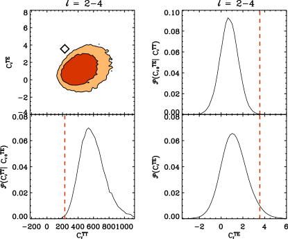
Figure 6.— Same as Figure 3, except assuming cosmic variance limited measurements and a complete suppression of the primordial power spectrum at wavenumbers $k<k_{\star}=3\times 10^{-4}\ {\rm Mpc}^{-1}$ (Cline, Crotty, & Lesgourgues, 2003).

6. Conclusions

The correlations between the temperature and polarization power spectra provide a powerful consistency check on CMB anisotropy measurements. Cosmic variance fluctuations should be correlated between power spectra. By assuming the best-fit cosmological model we have shown that the observed ${\cal C}_{\ell}^{TE}$ - ${\cal C}_{\ell}^{TT}$ data at $2\leq\ell\leq 4$ are alarmingly large outliers. Much has been made recently of the degree to which the ${\cal C}_{\ell}^{TT}$ data on these scales is anomalously low, but it is almost equally alarming that the ${\cal C}_{\ell}^{TT}$ is low and ${\cal C}_{\ell}^{TE}$ is apparently typical. In most realizations of the WMAP best-fit model with low ${\cal C}_{\ell}^{TT}$ on large scales, ${\cal C}_{\ell}^{TE}$ is also low. It is extremely unlikely to see ${\cal C}_{\ell}^{TE}$ as high as the measured value, given the low observed ${\cal C}_{\ell}^{TT}$ . This correlation is not currently included in likelihood analyses of CMB data, but should be relatively easy to incorporate in future work. Current estimates of the optical depth are likely biased low. Prescriptions for reducing the primordial quadrupole may have problems producing ${\cal C}_{\ell}^{TE}$ amplitudes as high as those that are observed on the largest angular scales, given the correlation between ${\cal C}_{\ell}^{TT}$ and ${\cal C}_{\ell}^{TE}$ .

Most of the other multipole bins up to $\ell<20$ in Figure 2 appear reasonably consistent with the best fit cosmological model. The $\ell=20-23$ bin is discrepant at nearly the same level in the ${\cal C}_{\ell}^{TT}$ power spectrum, but at current noise levels the degree of correlation between the measured ${\cal C}_{\ell}^{TE}$ and ${\cal C}_{\ell}^{TT}$ is negligible. The full four-year data of WMAP will help to improve these constraints. More accurate treatments of the errors and residual correlation due to the cut-sky will be possible. Furthermore, it would be particularly interesting to study the value of the probability ${\cal P}({\cal C}_{\ell}^{TE}|{\cal C}_{{\ell}0}^{TE})$ for various galactic cuts as a probe of the galactic contribution (D. Spergel, private communication). In the more distant future, data of the quality forecasted for the Planck satellite will provide even more powerful consistency checks on the best-fit cosmological model. More accurate modeling of the galactic emission will also certainly help to address those issues.

What would it mean if the observed statistics of the CMB do not appear to be consistent with the best fit cosmological model? The simplest explanation would be that at least one of the measured components is not purely cosmological in origin, possibly due to Galactic contamination. For example, removing the Galactic foreground appears to enhance the inferred quadrupole (de Oliveira-Costa et al. , 2004). The absence of foreground contamination would be an exciting indication of new physics.

References

- Bennett et al. (2003) Bennett, C.L., ApJS, 148, 1
- Bennett et al. (1996) Bennett, C.L., ApJ, 464, L1
- Bond (1995) Bond, J. R. 1995, Physical Review Letters, 74, 4369
- Bridle et al. (2003) Bridle, A., Lewis, A.M., Weller, J., Efstathiou, G. 2003, NewAr, 47, 8, 787
- Contaldi et al. (2003) Contaldi, C.R., Peloso, M., Kofman, L., Linde, A. 2003, JCAP, 07, 002
- Cline, Crotty, & Lesgourgues (2003) Cline, J. M., Crotty, P., & Lesgourgues, J. 2003, JCAP, 09, 010
- de Oliveira-Costa et al. (2004) de Oliveira-Costa, A., Tegmark, M., Zaldarriaga, M. & Hamilton, A. 2004, Phys. Rev. D, 69, 6, 063516
- Efstathiou (2003a) Efstathiou, G. 2003, Mon. Not. R. Astron. Soc., 343, 4, L95
- Efstathiou (2003b) Efstathiou, G. 2003, Mon. Not. R. Astron. Soc., 346, 2, L26
- Feng and Zhang (2003) Feng, B., and Zhang, X. 2003, Physics Letters B, 570, 3-4, 145
- Hinshaw et al. (2003) Hinshaw, G. et al. , ApJS, 148, 135
- Kaplinghat et al. (2003) Kaplinghat, M., et al. , 2003, ApJ, 583, 24
- Hu and Dodelson (2002) Hu, W., and Dodelson, S. 2002, ARA&A, 40, 171
- Jaffe (2003) Jaffe, A. H. 2003, NewAr, 47, 11, 1001
- Kogut et al. (2003) Kogut, A. et al. , ApJS, 148, 161
- Leitch et al. (2002) Leitch, E. M. et al. 2002, Nature, 420, 763
- Spergel et al. (2003) Spergel, D. et al. 2003, ApJS, 148, 175
- Tegmark & Zaldarriaga (2002) Tegmark, M. & Zaldarriaga, M. 2002, Phys. Rev. D, 66, 103508
- Tegmark et al. (2003) Tegmark, M., de Oliveira-Costa, A. & Hamilton, A. 2003, Phys. Rev. D, 68, 12, 123523
- Verde et al. (2003) Verde, L. et al. , ApJS, 148, 195; see also http://lambda.gsfc.nasa.gov for relevant data and routines
- Zaldarriaga (1997) Zaldarriaga, M. 1997, Phys. Rev. D, 55, 1822
- Zaldarriaga & Seljak (1997) Zaldarriaga, M. & Seljak, U. 1997, Phys. Rev. D, 55, 1830
- Zaldarriaga, Spergel, & Seljak (1997) Zaldarriaga, M., Spergel, D. N., & Seljak, U. 1997, ApJ, 488, 1