Morphology and kinematics of Lynds 1642

The high latitude translucent molecular cloud L1642 has been mapped in the J=1-0 and J=2-1 transitions of ¹²CO, ¹³CO and C¹⁸O using the SEST radio telescope. We have analysed the morphology and velocity structure of the cloud using the Positive Matrix Factorization (PMF) method. The results show that L1642 is composed of a main structure at radial velocity 0.2 km s^-1 while the higher velocity components at $\sim$0.5 and 1.0 km s^-1 form an incomplete ring around it, suggesting an expanding shell structure. Fainter emission extends to the north with a still higher velocity of up to 1.6 km s^-1. Such a velocity structure suggests an elongated morphology in the line of sight direction. The physical properties of the cloud have been investigated assuming LTE conditions, but non-LTE radiative transfer models are also constructed for the ¹³CO observations. We confirm that L1642 follows an $r^{-1}$ density distribution in its outer parts while the distribution is considerably flatter in the core. The cloud is close to virial equilibrium.
In an Appendix the PMF results are compared with the view obtained through the analysis of channel maps and by the use of Principal Component Analysis (PCA). Both PMF and PCA present the observations as a linear combination of basic spectral shapes that are extracted from the data. Comparison of the methods shows that the PMF method in particular is able to produce a presentation of the complex velocity that is both compact and easily interpreted.

1 Introduction

High latitude translucent molecular clouds are ideal targets for the study of the interactions between different phases of the interstellar medium which are subjected to the general interstellar radiation field. The visual extinction of these clouds is modest ($A_{V}\sim$1-3 mag) which places them between dark and diffuse clouds. As they are minimally affected by embedded star-formation the external radiation field is the dominant heating source. Furthermore, due to the high galactic latitude of the clouds, observations are seldom contaminated by foreground or background emission. The cloud L1642 (=MBM20) is a prototype of this class of clouds. It is located at galactic coordinates $l$=210.9$\degr$, $b$=-36.5$\degr$. The distance determination by Hearty et al. (hearty00 (2000)) places it between 112 and 160 pc. Based on X-ray measurements, Kuntz et al. (kuntz97 (1997)) suggested that L1642 is within or close to the edge of the local bubble, which in this direction is at about 140 pc according to Sfeir et al. (sfeir99 (1999)). This is in good agreement with the direct measurement and we adopt 140 pc for the distance of L1642. Based on previous multiwavelength data (Liljeström and Mattila liljestrom88 (1988); Taylor et al. taylor82 (1982); Laureijs et al. laureijs87 (1987); Liljeström liljestrom91 (1991)) L1642 appears as a cool and quiescent cloud. It is associated with a much larger HI cloud (over 4$\degr$) with cometary structure. This is also seen in the IRAS 100 $\mu$m image. The tail is perpendicular to the Galactic plane, and points towards the plane.

The IRAS point sources IRAS 04325-1419 and IRAS 04237-1419 make L1642 one of the closest star forming clouds. The source colours suggest that they are T-Tauri stars. In particular, IRAS 04237-1419 shows Herbig-Haro characteristics (Sandell et al. sandell87 (1987); Reipurth & Heathcote reipurth90 (1990)). However, the low luminosity of the source ($L<$0.6 L_⊙) means that it will have only a very local influence.

In this paper, we present an analysis of L1642, making use of new CO observations with a wider map area and/or denser grid than in the previous studies. After the description of observations in Sect. 2, Sect. 3 is devoted to the analysis of morphology and kinematics using the Positive Matrix Factorization method. The analysis is also carried out using another multivariate method, the Principal Component Analysis (Murtagh & Heck MH87 (1987)) and by channel maps. A comparison of the analysis methods and some comments on their relative strengths and weaknesses are given in an Appendix. In Sect. 4 we discuss the correlations between the observed lines, and in Sect. 5 the physical properties of the cloud are derived. Finally, in Sect. 6 we present our conclusions.

2 Observations and data reduction

Molecular line observations were made by K.L. in August 1999. The transitions J=1–0 and J=2–1 of ¹²CO, ¹³CO and C¹⁸O were observed with the Swedish-ESO Submillimetre Telescope (SEST). The receivers were cooled Schottky diode mixers operated in 80-116 GHz and 216-245 GHz bands. The channel separation of the AOS spectrometer was 0.11 km s^-1 for the $J$=1–0 transition and 0.06 km s^-1 for $J$=2–1 transition (Booth et al. booth89 (1989)). Observations were made in frequency switching mode. The calibration was done using the chopper-wheel method (Ulich & Haas ulich76 (1976)) and checked by observing the Orion KL nebula. Antenna temperatures ($T_{\rm A}^{\ast}$) were converted to radiation temperatures ($T_{\rm R}^{\ast}$) using the Moon efficiency. The half power beam widths are 45$\arcsec$ and 23$\arcsec$ for the 1-0 and 2-1 transitions, respectively. The grid spacing was 3$\arcmin$. The grid positions were planned to be identical to the map positions of our 200 $\mu$m ISOPHOT map (Lehtinen et al., in preparation).

Fig. 1 shows examples of observed line profiles. Typical noise levels were $\Delta T_{\rm rms}=$0.06 K for the C¹⁸O(2–1) spectra and $\sim$0.15 K for all the other transitions.

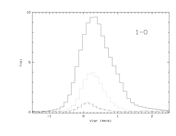
Figure 1: Averaged spectra observed towards the centre of L1642 (04h35m10.1s, -14$\degr$15’58” (J2000)). The solid, dotted and dashed histograms are respectively the ¹²CO, ¹³CO and C¹⁸O profiles.

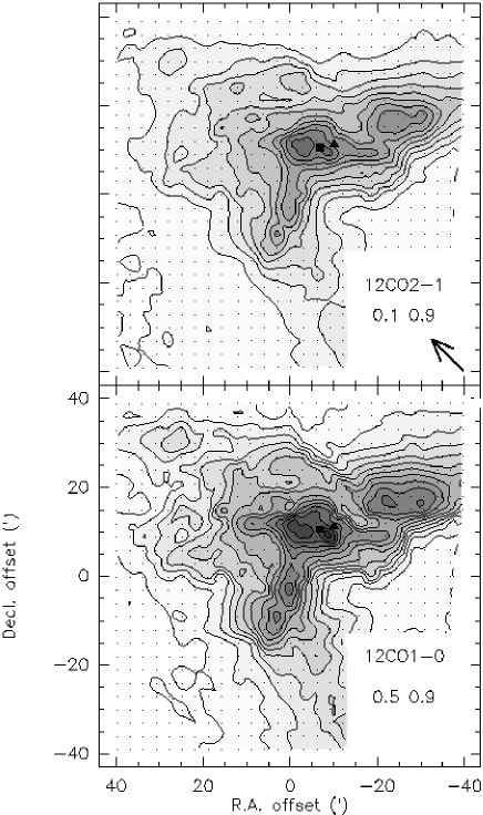
Figure 2: Contour maps of the ¹²CO line area. The square and the triangle indicate the position of IRAS 04327-1419 and IRAS 04325-1419, respectively. The two numbers given for each map are the isocontour starting values and the steps in K km s^-1. The centre position (0,0) is 04h35m30s, -14$\degr$24$\arcmin$28$\arcsec$ (J2000). The arrow indicates the direction of the cloud tail seen in HI and IRAS maps

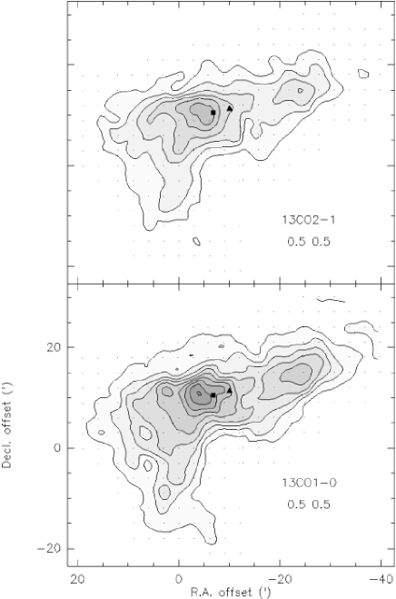
Figure 3: As in Fig.2, but for ¹³CO

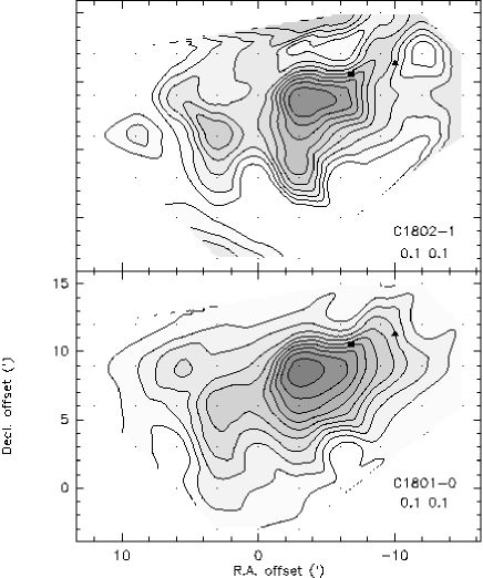
Figure 4: As in Fig.2, but for C¹⁸O

3 Morphological and kinematic analysis

The observed line area maps are presented in Figs. 2-4. We utilize the multi-line information to probe the cloud morphology and kinematics from the dense central parts, as traced by the C¹⁸O, to the diffuse outer parts, as traced by ¹²CO. The conventional channel maps as well as the results from principal component analysis (PCA; see e.g. Murtagh & Heck MH87 (1987)) are given in Appendix A. Here we study the cloud structure by using Positive Matrix Factorization (PMF), since comparison with the other methods showed that this method gives the most compact presentation for the complex cloud structure. The different analysis methods were not only used to study this particular cloud, Lynds 1642, but also to evaluate the relative merits of the methods. These are discussed in Appendix A.3.

3.1 Positive Matrix Factorization

The Positive Matrix Factorization (PMF) method assumes the spectra to be the sum of a few basic velocity components. The line decomposition computes the shape and intensity of each component imposing positivity to their profile. The application of PMF to the analysis of molecular lines was largely discussed by Juvela et al.(juvela96 (1996)) and we repeat here only some of the main points. Let $X$ be the data matrix and $\Sigma$ a matrix consisting of estimated standard deviations of the elements of $X$. Both matrices have dimensions $n\times m$. Given matrices $X$ and $\Sigma$ and the rank of factorisation, $r$, PMF calculates a factorisation

$$X=GF+E,G_{ik}\geq 0,F_{kj}\geq 0$$ (1)

with $i$=1,…,$n$, $k$=1,…,$r$ and $j$=1,…,$m$). $E$ is the residual matrix and factor matrices $G$ and $F$ are selected to minimise its weighted norm

$$Q=\sum_{i,j}(E_{i,j}/\Sigma_{i,j})^{2}=\sum_{i,j}(\frac{(X-GF)_{ij}}{\Sigma_{ij}})^{2}.$$ (2)

The rank $r$ equals the number of spectral components used in approximating the observed data.

There are two essential improvements over PCA analysis (see Appendix A.2). Firstly, the elements of the factor matrices, $G$ and $F$ are required to be positive. In this case, this is a physically meaningful assumption. The observed spectra are decomposed into positive spectral components and a direct interpretation of the results will be easier than in the case of PCA, where profiles may contain as many negative as positive values. Secondly, the residuals are weighted according to individual error estimates of the observations. This makes it possible to use all observations without the risk that results will be unduly affected by individual, low signal-to-noise ratio spectra. Like PCA, the PMF method regards the observations as a sum of emission components at fixed radial velocities. In the case of continuous velocity gradients, this is not an exact description of the data, and this must be kept in mind when interpreting the results.

PMF requires the selection of the number of components, $r$, and a suitable value of $r$ could be determined e.g. based on the eigenvalues of matrix $X$. In practise, it is better to try different $r$-values and select the best value based on the $Q$-values obtained and the appearance of the components and the residual maps. The PMF method was run independently on the ¹³CO(1-0), ¹³CO(2-1), ¹²CO(1-0), ¹²CO(2-1), C¹⁸O(1-0) and C¹⁸O(2-1) datasets to extract kinematic information for L1642. Factorisations were computed for ranks $r$=1 to $r$=5 using the Multilinear Engine program (Paatero paatero99 (1999)). Results of factorisations with $r=4$ are shown in Figs. 5– 7. The figures show the computed spectral profiles of the components for $J$=1-0 lines and their spatial distribution over the mapped area. The results for the $J$=2-1 transitions were very similar to those of $J$=1-0. By trying decomposition with 1 to 5 components, we found that, in ¹²CO and ¹³CO, 4 components are enough to describe the main kinematic structures. For C¹⁸O, only three significant components were found, but 4 components are shown for the sake of completeness.

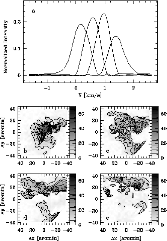
Figure 5: Result of the PMF factorisation of ¹²CO(1–0) observations with four spectral components. The spectral profiles of the components are shown in the first frame. The other frames show the intensity distribution of the components over the observed map. The component maps are in the order of increasing radial velocity of the component

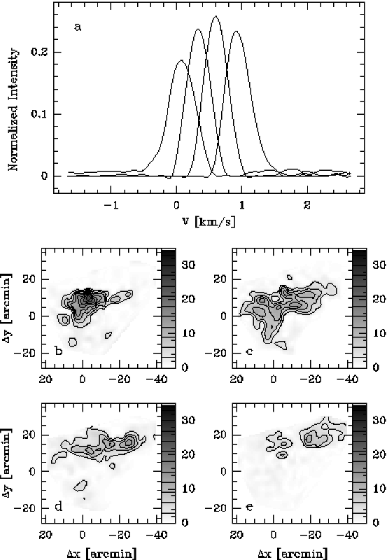
Figure 6: Result of the PMF factorisation of ¹³CO(1–0) observations with four components

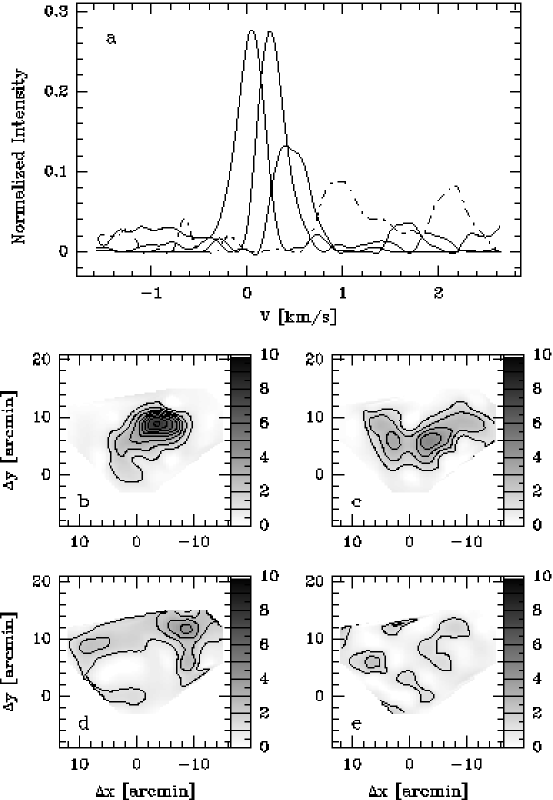
Figure 7: Result of the PMF factorisation of C¹⁸O(1–0) observations with four components. The last component is mostly noise and is drawn with dashed line

3.2 Cloud kinematics and environmental effects

We analyse the kinematic structure of L1642 using the PMF results shown in Figs. 5-7. The maps of the kinematic components show an intricate structure. Most of observed CO lines are not pure gaussians, but exhibit small shoulders and slightly flattened tops (see Fig. 1). The possible causes for such line asymmetries are: ejection, contraction, rotation, self absorption, saturation, or superposition of several kinematically separate cloud fragments along the line of sight.

3.2.1 ¹²CO lines

With $r=4$, the first component of PMF decomposition traces the central part of L1642. The second one indicates strong emission south of the centre, extending to the south west edge of the map. This is still visible in the third component. However, the last two components mostly trace emission from the northern part, indicating a velocity gradient towards the north, or possibly the presence of another cloud component at a higher radial velocity. The decomposition shows patchy emission at $\sim$1.25 km s^-1, most notably the prominent clump at (-20$\arcmin$,+20$\arcmin$) embedded in more extended emission at $\sim$0.4 km s^-1. With more components ($r$=5), the $Q$-value improves further by more than 15%, and decompositions show more details of the velocity structure in the northern part. The general kinematic structure is clear, but it cannot be interpreted directly e.g. as simple rotation, contraction or expansion. The smallest-velocity component 1, centred at $\sim$0.2 km s^-1, delineates the maximum CO emission core of the cloud. At higher radial velocities (components 2 and 3) emission in both northern and southern parts of the maps can be seen. The highest-velocity component 4 is only present in the extreme North.

Its velocity difference of $\sim$1.3 km s^-1 with respect to the cloud core corresponds to a distance of $\sim$1 pc travelled in 10⁶ years, a typical timescale for cloud dynamics.

The residual maps of PMF factorizations with $r$=4 (and with $r$=5) are very similar for the two ¹²CO transitions, and both show several clear clumps, most notably at positions (0$\arcmin$, 9$\arcmin$) and (-21$\arcmin$, 21$\arcmin$). There is also a wider area of large residuals between these positions, at around (-10$\arcmin$, +10$\arcmin$), i.e. around the position of the source IRAS 04325-1419, which is associated with an outflow (Liljeström et al. liljestrom89 (1989)).

The study of residuals is a very powerful tool for finding deviating spectra. By subtracting the decomposition from the observation matrix one can not only identify deviating spectra, but also see exactly how the profiles differ. For example, two distinct structures were observed in the PMF residual maps of both ¹²CO(1–0) and ¹²CO(2–1). Around position (0$\arcmin$, 9$\arcmin$) the spectra show clear blueshifted excess ($v\sim$-0.5 km s^-1), while around position (-21$\arcmin$, 21$\arcmin$) the excess is as clearly redshifted ($v\sim$+1.3 km s^-1) (see Fig.8). These residual features are quite strong, with peak ¹²CO(1–0) antenna temperature above 1 K. Corresponding features can even be detected in channel maps. However, the PMF analysis indicates that the emission seen in the -0.5 km s^-1 channel is not a normal tail of the stronger emission at higher velocities. The spectra at the given position have distinctly different profiles.

Figure 8: Observed ¹²CO(1–0) and ¹³CO(1–0) spectra (upper frames) and the residuals (lower frames) of the PMF fit at positions (0$\arcmin$, 9$\arcmin$) and (-21$\arcmin$,21$\arcmin$). The ¹²CO spectra are drawn with thicker lines

3.2.2 ¹³CO lines

The ¹³CO emission is less extended, but it exhibits similar kinematics as ¹²CO. Figure 6 shows the ¹³CO(1-0) decomposition with $r$=4. The maps for the transition $J$=2-1 are again very similar. The first component is concentrated in the cloud centre, while the last one traces emission in the north, in particular the two clumps at (-20$\arcmin$, +20$\arcmin$) and (-5$\arcmin$, +15$\arcmin$), already seen in the ¹²CO maps. On the other hand, the ridge of emission south of the centre is weak in ¹³CO. For ¹³CO(1-0), a change from $r$=1 to $r$=2 decreases $Q$ by 35$\%$, while the drop is only 15$\%$ in the case of ¹³CO(2-1). A similar difference is noted for higher $r$-values. This is caused by the difference in the signal-to-noise ratio, and with $r>3$, some noise ripples appear in the ¹³CO(2-1) components. As in the case of ¹²CO residual maps, the ¹³CO(1-0) maps show significant residual emission, e.g. around position(0$\arcmin$,+9$\arcmin$) (see Fig. 8).

3.2.3 C¹⁸O lines

C¹⁸O probes the deepest and densest parts of L1642. Compared with the previous lines, it is spatially much more concentrated and is restricted to a velocity range between -0.3 and 0.5 km s^-1. The PMF 1-component decomposition of the C¹⁸O(1-0) shows that the emission has a mean velocity of 0.2 km s ^-1 and a width of 0.47 km s^-1. We show in Fig. 7 the decomposition with $r=4$ for completeness, even if decompositions with $r>3$ have some irregular components that are caused mostly by noise. For the two transitions, the maps of the first three components agree with each other and these are therefore likely to be real emission features. At low radial velocities, a core located at (-4$\arcmin$, +9$\arcmin$) is the main feature. At intermediate velocities, two separate clumps appear at (+3$\arcmin$, +5$\arcmin$) and (-4$\arcmin$, +6$\arcmin$). The third component shows some emission north of the core, and, in the maps of both transitions, weak clumps are seen at (-9$\arcmin$, +12$\arcmin$) and (+7$\arcmin$, +9$\arcmin$). The last components have completely different distributions and spectral profiles and, and therefore are unlikely to be related to actual cloud structure. Like residual maps, these ‘noise factors’ can be used to check for systematic errors or artifacts in data. For example, in the case of C¹⁸O(2-1), the fourth spectral component is almost flat and positive, suggesting bad baseline fits in a few spectra. The two IRAS sources do not coincide with the main peak of the C¹⁸O emission, but are located inside the western clump seen in the third component map, i.e. around velocity $\sim$0.3 km s^-1.

In addition to the clumps already mentioned, there are separate patches of emission that are seen in the second and the third component maps. They can be either independent clumps or parts of a more continuous density distribution containing gas motions along the line of sight. The latter hypothesis seems more likely, because the features do not have a clear counterpart on peak intensity and line area maps.

3.2.4 Summary of kinematics and environmental effects

To summarise, PMF (with increasing $r$) provides a hierarchical view of the cloud kinematics. Firstly, the main cloud is distinguished from the emissions in the north. Secondly, kinematic substructures appear in the northern part, and finally, kinematic substructures are identified inside the central area of L1642. The northern part is likely to belong to L1642, since the velocity difference is less than the typical velocity dispersion of molecular clouds (the typical cloud-to-cloud velocity dispersion is 7$\pm$1.5 km s^-1, according to Blitz and Fich, blitz83 (1983)). The ¹²CO observations show a systematic velocity structure with the main emission at $\sim$0.2 km s^-1 (a velocity close to that of the C¹⁸O core), and fainter and patchy emission with velocities up to 1.6 km s^-1 extending to the north and to the south.

In the PMF decompositions of the ¹²CO lines the first component shows the compact core. The second component shows almost a ring-like structure at $\sim$0.5 km s^-1 higher radial velocity. This is illustrated in Fig. 9a where we have overlayed the contours of the first two PMF components. Similar structure is seen in the decomposition of the ¹³CO(1-0) observations (see Fig. 9b). This suggests some kind of an expansion. At higher velocities, no emission is seen towards the centre of the cloud. Therefore, the structure cannot be spherically symmetric, but it could be an incomplete expanding shell, the far side of which is missing.

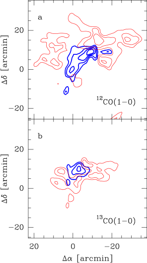
Figure 9: The spatial distributions of the first two PMF components in the case of the ¹²CO(1-0) and the ¹³CO(1-0) observations. The blue and red contours correspond to the first and the second PMF component, respectively, as shown in Figs. 5 and 6. The contour levels are 40, 50, and 55 for the first and 20, 25, and 30 for the second ¹²CO component, and 14, 19, and 24 for the first and 8.5 and 11.5 for the second ¹³CO component. The units are the same as used in Figs. 5 and 6.

The L1642 cloud is the head of a large cometary structure with a tail extending more than 5 degrees in the north eastern direction. The tail is seen very clearly, e.g. in the 100$\mu$m IRAS map. Furthermore, HI data shows a velocity gradient along the tail, with increasing velocity towards the north-east (Taylor et al. taylor82 (1982)). This suggests that the first PMF component represents the very head of the whole structure, and gas in the head is flowing relative to the rest of the structure, not only towards the south-west but also more towards us. The second PMF component would correspond to more diffuse material being left behind by the moving cloud core. In the north-eastern corner, the spatial separation of the third and fourth PMF components indicates a velocity gradient across the tail. This velocity gradient closely agrees with the HI velocity structure (Liljeström & Mattila liljestrom88 (1988); Taylor et al. taylor82 (1982)) indicating that the atomic and molecular gas components are well mixed in the cloud.

In projection on the sky, L1642 is located in the direction of the edge of the Orion-Eridanus Bubble, and we must consider the possibility of their interaction. ¿From multi-wavelength analysis, Reynolds and Odgen (reynolds79 (1979)) have shown that the Orion-Eridanus Bubble is an expanding cavity (expansion velocity $\sim$15 km s^-1) full of warm ionised gas surrounded by an expanding HI shell. X-ray enhancements have been measured and attributed to hot gas flowing out from the bubble through a chimney or a hole where L1642 would be located (Heiles et al. heiles99 (1999)). From HI data (Brown et al. brown95 (1995)), the bubble velocities range between -40 and +40 km s^-1. The largest spatial extension occurs between -1 and +8 km s^-1, which is the most probable range for the systematic velocity of the bubble. L1642 falls in the velocity range of the Orion-Eridanus Bubble, which suggests that it could have been swept up and hence shaped by the bubble. This would favour the hypothesis that the tail is formed as a stationary cloud embedded in moving interstellar medium. On HI maps (Brown et al. brown95 (1995)), L1642 appears isolated for velocities between -1.5 to 2.5 km s^-1. At these velocities, the bubble edges delineate an ‘empty space’ roughly centered on L1642. More precisely, L1642 is kinematically disconnected from the filaments at $l\sim$210$\degr$ which have velocities less than -3 km s^-1.

4 Correlations of the line intensities

We use the multi-transition information to examine the excitation conditions of L1642. There is a good correlation between the integrated line intensities of the $J=$2–1 and $J=$1–0 transitions (Fig. 10). The following relations are obtained for the line areas:

$$W[^{12}{\rm CO(2-1)}] =(0.75\pm 0.06)\,\,W[^{12}{\rm CO(1-0)}]$$

$$-(0.12\pm 0.40)$$

$$W[^{13}{\rm CO(2-1)}] =(0.71\pm 0.01)\,\,W[^{13}{\rm CO(1-0)}]$$

$$-(0.01\pm 0.19)$$

These relations are in agreement with other high latitude clouds (e.g. Ingalls et al. ingalls00 (2000)). The ¹²CO/¹³CO ratio is much smaller than the typical relative abundance of the species, which is a natural consequence of ¹²CO being optically thick.

Figure 10: Correlation between ¹²CO $J=$2–1 and $J=$1–0 line areas

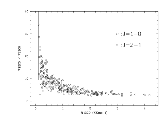
Figure 11: W[¹²CO]/W[¹³CO] versus W[¹³CO]

The decrease of $W[^{12}$CO]/W[¹³CO] versus W[¹³CO] (Fig. 11) is caused by the saturation of the CO line. The few high ratio points at low $W[^{13}$CO] are attributed to the case in which both isotopes are optically thin and the asymptotic value of about 3 is reached when ¹³CO becomes optically thick. These small ratios are found in the central parts of the cloud.

The mean value of the ratio $W$[¹³CO(1-0)]/$W$[C¹⁸O(1-0)] is 7.2$\pm$0.3. Within a central region of some 10$\arcmin$$\times$15$\arcmin$ the ratio decreases, presumably due to ¹³CO saturation, below the normally assumed isotopic abundance ratio of 5.5. On the other hand, everywhere in the outer region of the area covered by C¹⁸O observations the ratio increases to almost 10. Although ¹³CO emission is still not completely optically thin, the observed variation also indicates a change in the relative abundance of the two species. The ¹³CO/C¹⁸O ratio is enhanced to values $>$5.5 by ¹³CO fractionation. The average ratio for the corresponding $J=$2–1 lines is 6.8$\pm$2.2.

5 Column density distribution and mass of L1642

5.1 LTE-analysis

In order to calculate the column density, one must first determine the excitation temperature throughout the cloud. The standard methods assume LTE conditions, and either ¹²CO is assumed to be optically thick, or the optical depth ratio of two isotopic lines is assumed equal to the terrestrial abundance ratio (the assumed ¹²CO to ¹³CO abundance ratio is $\sim$89). In addition, an identical excitation temperature is usually assumed for both isotopes.

In our case, both methods agree up to distances of $\sim$30$\arcmin$ from the cloud centre (the adopted cloud center is: -5$\arcmin$, +10$\arcmin$), after which the ¹³CO antenna temperature values are affected by noise.

The excitation temperature has a nearly constant value from cloud centre to edge (Fig. 12).

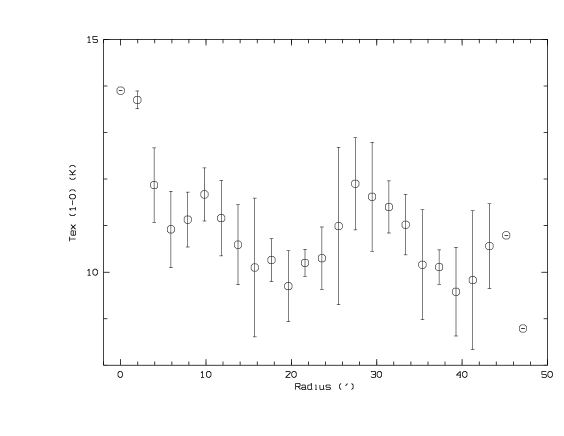
Figure 12: Excitation temperature $T_{\rm ex}$(1–0), calculated from ¹³CO/¹²CO peak antenna temperature ratio, versus radius. Error bars reflect dispersion in each distance bin

In the central part of the cloud, ¹²CO and ¹³CO emission lines are certainly optically thick, and hence the derived temperature may not be representative of the bulk of the cloud. The best temperature estimate for the cloud centre is obtained from the ¹³CO/C¹⁸O ratio which gives a value of $T_{\rm ex}$=8 K. Based on the optically thick ¹²CO emission, the mean temperature estimate is $T_{\rm ex}$=10.7 K.

The column densities and the cloud mass were estimated based on the ¹³CO data. The estimates are derived from the $J$=1–0 line, since according to radiative transfer models (see Appendix B.2) this gives more reliable estimates than the $J$=2–1 transition.

For LTE calculations, we assume a constant excitation temperature of 10K. Figure 13 shows the H₂ column density map derived from ¹³CO(1–0). The adopted conversion factor is N(H₂)/ N(¹³CO)=1 10⁶. IRAS 04237-1419 is close to the column density maximum, while IRAS 04325-1419 is located half way to the edge of the central core. The H₂ column density was averaged in concentric rings of angular radius $r$ from the centre, and the resulting radial column density distribution is shown in Fig. 14. The vertical error bars represent the dispersion of the values averaged at each radius. An $r^{-1}$ distribution is obtained in the outer parts of the ¹³CO cloud ($r>$5.6$\arcmin$), but the distribution in the core ($r<$5.6$\arcmin$) is significantly flatter. Such behaviour is commonly observed in cloud cores (Bacmann et al.,bacmann00 (2000); Ward-Thompson et al., ward94 (1994), ward99 (1999)), and is in good agreement with both the previous ¹³CO observations of L1642 (Liljeström, liljestrom91 (1991), see her Fig. 7) and the density profile of dust (Laureijs et al. laureijs87 (1987)).

The cloud mass can be calculated according to

$$M(M_{\odot})=5.74\,10^{-20}\,d_{100pc}^{2}\int\int N(H_{2})\cos\delta\,d\delta\,d\alpha,$$ (4)

where $d_{100pc}$=$d$/100 pc, with $d$ the distance of the cloud. Within the boundary $T_{\rm R}^{\ast}(^{13}{\rm CO}(1-0))\geq 1$ K, corresponding to $H({\rm H}_{2})\geq 6\times 10^{20}$ cm^-2, we obtain from the $N$(H₂) map as shown in Fig. 13 $M=(30\pm 10)\,M_{\odot}\,d_{100pc}^{2}\sim 59\,M_{\odot}$ (assuming $d$=140 pc).

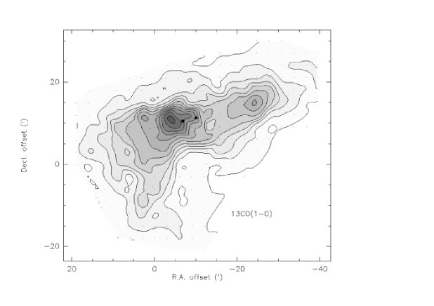
Figure 13: Map of H₂ column density derived from ¹³CO(1-0) lines assuming LTE. The contours range from 1.0 10²⁰ to 5.6 10²¹ cm^-2 by 5.0 10²⁰ cm^-2. The filled square and the triangle indicate the positions of IRAS 04237-1419 and IRAS 04325-1419

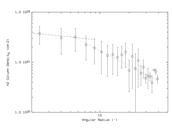
Figure 14: The profile of the H₂ column density derived from ¹³CO(1-0) observations. The dotted lines are for r^-1 trends and dashed lines for r^-0.2. The centre is at $\Delta\alpha$=-5$\arcmin$, $\Delta\delta$=+10$\arcmin$ (see Fig. 13)

5.2 Spherically symmetric non-LTE models

In reality, the excitation temperature is not likely to be constant over the whole line of sight. This may lead to erroneous results in the normal LTE analysis, especially at low temperatures (e.g. Padoan et al. padoan00 (2000)). For this reason, we compared the LTE results, as described above, with non-LTE radiative transfer calculations. The comparison gives an estimate for the uncertainty of the results. Precise determination of the cloud mass requires detailed knowledge of the density and temperature distributions.

The ¹³CO observations were modelled with a spherically symmetric cloud with radial density distribution $n\sim r^{-2.0}$, except for the central 10% of the cloud radius for which constant density was adopted. The density contrast between the centre and the cloud surface was set to 20. The radiative transfer problem was solved with a Monte Carlo method (Juvela juvela97 (1997)), and the results were compared with observed spectra which were averaged over concentric annuli. The density and the size of the model cloud were varied in order to find parameter values that best reproduced the observations. A value of 1.0$\cdot$10^-6 was assumed for the fractional abundance of ¹³CO.

Isothermal models with $T_{\rm kin}$ between 8 and 14 K were first considered. The $\chi^{2}$ values were practically independent of the temperature and it is clear that the temperature cannot be well constrained based on ¹³CO observations alone. The mass estimates ranged from 82 M_☉ at 8 K to $\sim$65 M_☉ at 14 K. The intensity ratio between the 2-1 and 1-0 lines was generally too low and, as expected for a microturbulent model, the line profiles toward the centre positions were strongly self-absorbed.

We further studied a set of models in which the kinetic temperature increase linearly with the radius. These did not lead to significantly better fits but the mass estimates were slightly lower and close to the LTE values. For a model where $T_{\rm kin}$ increases from 9 K in the centre to 14 K on the cloud surface, the estimated mass was 61 $M_{\sun}$ and the central density was 1.2$\cdot$10⁴ cm³. For this model the fitted spectra are shown in Fig. 15.

As can be seen the spherically symmetric models do not provide a good fit to the observations. At the centre position the observed spectra are clearly asymmetric and when observations are averaged over concentric annuli the presence of different velocity components or gradients leads to artificial line broadening or even multiple peaks in the averaged profiles. Such effects can be taken into account only in three-dimensional models (see Sect. 5.3 add Appendix B). The main shortcoming of the spherically symmetric models is, however, the low line ratio between the $J$=2-1 and $J$=1-0 transitions. This could indicate either a much higher kinetic temperature, significant foreground absorption or more likely density inhomogeneities inside the source.

Figure 15: Spectra from a spherically symmetric model cloud (solid lines) and observed spectra (histograms) averaged over different annuli centred at the position 4h35m13.6s -14$\degr$15$\arcmin$28$\arcsec$. In the model the kinetic temperature increased linearly from 9 K in the centre to 14 K on the cloud surface. The radius of the annulus is given in each frame. Thick lines represent ¹³CO(1-0) and thin lines ¹³CO(2-1) spectra.

The observed average intensity ratio ¹³CO(2-1)/¹³CO(1-0) is 0.69 (the average of observations with W(¹³CO(1-0))$>$1 K km s^-1). Assuming LTE conditions, constant excitation along the line of sight, and an excitation temperature of $T_{\rm ex}$=10 K (Fig. 12), such a ratio would imply an optical depth of ¹³CO(2-1)$\approx$2. The ¹³CO molecule is, however, not thermalized. In our calculations, the excitation temperature of the 2–1 transition is always clearly below that of the transition 1–0. For example, in the centre of the model cloud with $T_{\rm kin}$=12K the difference is almost three degrees. At higher densities ¹³CO would become less subthermally excited and the ratio ¹³CO(2-1)/¹³CO(1-0) would increase. Therefore, the observed high line ratios may indicate that the cloud is inhomogeneous and ¹³CO is partly thermalized in spite of the low average density.

5.3 Three-dimensional non-LTE models

The line profiles from a real, turbulent cloud are seldom as clearly self-absorbed as in the microturbulent models. The cloud was therefore also modelled with fully three-dimensional models. In these isothermal models, the general density distribution was based on the LTE column density maps. Details of the calculations are given in Appendix B.1. The best fit was obtained at a significantly lower temperature than for the spherical homogeneous models, $T_{\rm kin}$=8 K, leading to a mass estimate of 70 $M_{\sun}$. However, the temperature cannot be accurately determined, and for the model with $T_{\rm kin}$=14 K, the average line ratio, ¹³CO(2-1)/¹³CO(1-0)=0.63, is still reasonably close to the observed value of 0.69. For any given temperature, the predicted mass values were only slightly lower than in the spherical models.

We applied a standard LTE analysis to the spectra produced by the 3D models. This analysis showed that, in the parameter range considered here, the LTE column density estimates based on the 1–0 are reliable (see Appendix B.2). The mass estimate from the LTE-calculations are indeed consistent with the 3-D modelling, when a kinetic temperature of $T_{\rm kin}\sim 12\,$K is assumed.

5.4 Dynamical state of the cloud core

We investigate the dynamical state of L1642, following the method by Liljeström (liljestrom91 (1991)), who estimated the ratio $\frac{\sigma_{\rm gas}}{\sigma_{\rm vir}}$ where $\sigma_{\rm gas}$ and $\sigma_{\rm vir}$ are the velocity dispersion of the gas derived from observation and the virialized velocity dispersion of the mean gas particle, respectively. The effective radius of the cloud is $R_{\rm eff}=0.97\,d_{100pc}$ pc ($R_{\rm eff}=\sqrt{ab}$; $a$=semi-major axis, $b$=semi-minor axis). A value of $\sigma_{\rm gas}$=0.17 km s^-1 is obtained from the ¹³CO line width (corrected for instrumental and line opacity broadening). Adopting $T_{\rm kin}$=12 K and assuming $d$=140pc, we find $\sigma_{\rm vir,1-dim}$=0.21$\pm$0.02 and hence a ratio of $\frac{\sigma_{\rm gas}}{\sigma_{\rm vir}}$=0.81$\pm$0.08 for a homogeneous sphere. For a centrally condensed sphere with $n\propto r^{-1}$, we obtain ${\sigma_{\rm vir}}$=0.19$\pm$0.02 and $\frac{\sigma_{\rm gas}}{\sigma_{\rm vir}}$=0.89$\pm$0.08. The values are very close to 1, suggesting that the cloud is probably in virial equilibrium. Wed note, that ¹³CO traces only some 80% of the total cloud mass (e.g. Falgarone and Puget, falgarone88 (1988)), while another 20% is in more diffuse cloud medium.

6 Conclusions

We have presented ¹²CO, ¹³CO and C¹⁸O $J$=1–0 and $J$=2–1 line observations of the translucent high latitude cloud L1642. The main results of this study are summarized as follows:

- Besides the conventional channel maps, we have also applied the Principal Component Analysis (PCA) and Positive Matrix Factorization (PMF). The PMF method was found to produce an easily understandable, compressed presentation of the data that preserved all the important morphological and kinematic features of the cloud.

- The morphological and kinematic analysis has shown a main structure at a velocity of 0.2 km s^-1 with an incomplete ring structure around it at larger velocities. Fainter emission extends to the north with velocities up to 1.6 km s^-1.

This structure suggests an incomplete expanding shell, the front side of which is seen in the main component.

An elongated morphology in the line of sight direction is also suggested by the kinematics.

- In C¹⁸O, only two spatially well separated clumps can be distinguished. These structures do not coincide with the two embedded IRAS sources, which are offset by 5–7$\arcmin$ from the main peak.

- We confirm that L1642 follows an $r^{-1}$ density distribution in its outer parts and a flatter distribution with $n\propto r^{-0.2}$ for the core. The cloud is probably in virial equilibrium.

- The LTE estimate of the cloud mass is 59 $M_{\sun}$.

- We performed three-dimensional radiative transfer modelling of the ¹³CO observations and obtained a cloud mass estimate of $\sim$70 $M_{\sun}$. The cloud temperature is, however, not well constrained, leading to large uncertainties in the mass estimates.

Appendix A Alternative methods for the study of cloud kinematics

A.1 Channel maps

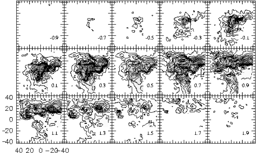
Figure 16: ¹²CO(1–0) channel maps. The velocity (in  km s^-1) is indicated on each panel. The contour interval is 0.3 K km s^-1 and the first contour is at 0.2 K km s^-1

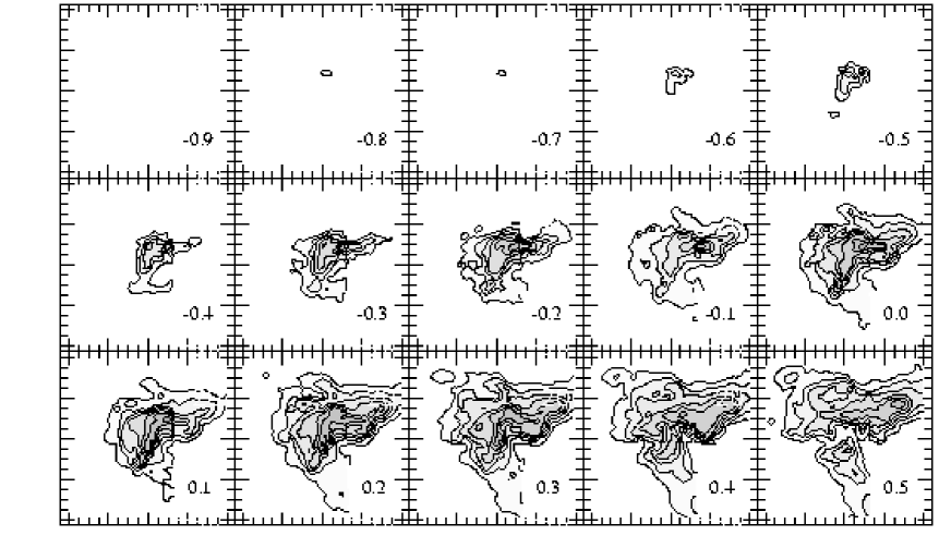
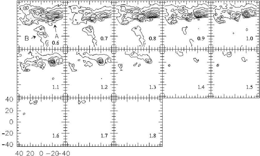
Figure 17: ¹²CO(2–1) channel maps. The velocity (in  km s^-1) is indicated on each panel. The contour interval is 0.2 K km s^-1 and first contour is at 0.2 K km s^-1. On this figure, structures A and B, mentioned in the text, are indicated on the 0.6 km s^-1 channel

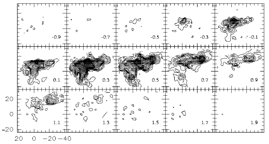
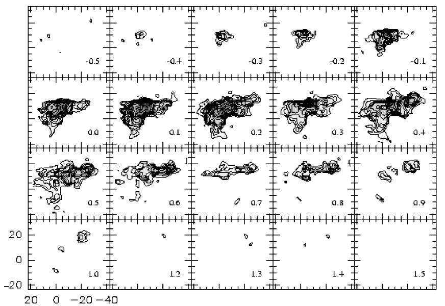
Figure 18: ¹³CO(1–0) (upper) and ¹³CO(2–1) (lower) channel maps. The velocity (in  km s^-1) is indicated on each panel. The contour interval is 0.1 K km s^-1 for 1–0 and 0.05 K km s^-1 for 2–1, both starting at 0.1 K km s^-1

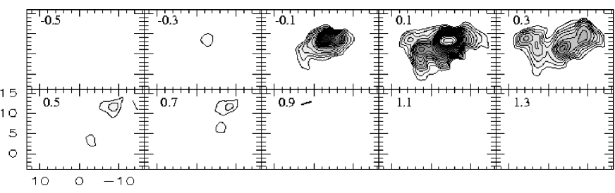
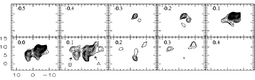
Figure 19: C¹⁸O(1–0) (upper) and C¹⁸O(2–1) (lower) channel maps. The velocity (in  km s^-1) is indicated on each panel. The contour interval is 0.03 K km s^-1 for 1–0 and 0.02 K km s^-1 for 2–1, the lowest contour lying at 0.1 K km s^-1

The ¹²CO, ¹³CO and C¹⁸O channel maps are shown in Figs. 16 to 19. In ¹²CO, the first significant emission appears at -0.5 km s^-1 around position (-3$\arcmin$, +10$\arcmin$) and, as the velocity increases, emission extends towards both south and west. Above -0.1 km s^-1, the general morphology remains the same with only small additional patches appearing. These suggest the presence of small internal motions and clumpy structure. Finally, above 0.5 km s^-1, the cloud breaks up into two separate structures. The first one (structure A; see Fig. 17) is elongated in the east-west direction and is located around $\Delta y\sim$20$\arcmin$. The second one (structure B) extends from the centre towards the south.

Structure A remains smooth between 0.6 and 0.9 km s^-1. At higher velocity, it fragments with persistent clumps at (-20$\arcmin$, +20$\arcmin$) and (+32$\arcmin$, +15$\arcmin$). The latter is well identified in ¹²CO(1–0) but is less clear in ¹²CO(2–1). The velocity of these clumps is $\sim$1.2 km s^-1. Structure B fades after 1 km s^-1, the mean velocity being $\sim$0.8 km s^-1. At higher velocities, the main structure is a faint elongated emission emanating from the (-20$\arcmin$, +20$\arcmin$) clump.

Fig. 20 shows the velocity diagram for ¹²CO(1–0) observations along the line between positions (40$\arcmin$,-40$\arcmin$) and (-40$\arcmin$,40$\arcmin$). The average velocity increases from $\sim$0.3 km s^-1 in the south to $\sim$1 km s^-1 at the northern end where the velocity increases all the way to the edge of the map. The three preeminent clumps at $\sim$(0$\arcmin$, 0$\arcmin$), (-10$\arcmin$, +10$\arcmin$) and (-20$\arcmin$, +20$\arcmin$) are visible as separate maxima. However, only the last one (at offset 30$\arcmin$ in Fig. 20) is clearly separated from the main cloud based on its radial velocity. The gradual change between offsets 15$\arcmin$ and 30$\arcmin$ does not necessarily require a continuous velocity gradient but could be caused by the superposition of emission at two separate velocities. The range of velocities is large, both at the location of the northern clump at (-20$\arcmin$, +20$\arcmin$) (offset +30$\arcmin$) and in the south (offset -15$\arcmin$). However, the largest dispersion is found at offset $7\arcmin$ where the emission extends to high positive radial velocities, especially compared with the velocity of the main emission. The location is some 5$\arcmin$ from IRAS 04325-1419, the source of a known outflow (Liljeström et al. liljestrom89 (1989)).

Figure 20: Velocity diagram of ¹²CO(1–0) observations along the line from position (40$\arcmin$,-40$\arcmin$) to (-40$\arcmin$,40$\arcmin$).

The ¹³CO emission is less extended, but it exhibits similar kinematics as ¹²CO. In ¹³CO(2–1), map emission clumps are clearly seen around (+6$\arcmin$, +12$\arcmin$), (-6$\arcmin$, +11.5$\arcmin$) and (+9$\arcmin$, -2$\arcmin$). The (-20$\arcmin$, +20$\arcmin$) emission clump is still dominant, with a mean velocity at around 0.8 km s^-1.

C¹⁸O probes the deepest and densest parts of L1642. Compared with the ¹²CO and ¹³CO lines, it is spatially much more concentrated and is restricted to a velocity range between -0.3 and 0.5 km s^-1. The emission mostly occurs around $\sim$0.15 km s^-1. Two main parts can be distinguished around $\Delta x\sim$-5$\arcmin$ (part A) and $\Delta x\sim$3$\arcmin$ (part B) (see Fig. 19). Both have several patches appearing at different velocities: in A at (-4$\arcmin$, +9$\arcmin$) ($V_{\rm lsr}\sim$-0.1 km s^-1), (-6$\arcmin$, +9$\arcmin$) ($V_{\rm lsr}\sim$0.1 km s^-1), (-4$\arcmin$, +6$\arcmin$) ($V_{\rm lsr}\sim$0.15 km s^-1) and (-4$\arcmin$, +3.5$\arcmin$) ($V_{\rm lsr}\sim$0.25 km s^-1), and in part B at (+2$\arcmin$, +6$\arcmin$) ($V_{\rm lsr}\sim$0.1 km s^-1) and (+6$\arcmin$,+9$\arcmin$) ($V_{\rm lsr}\sim$0.3 km s^-1). These could either be independent clumps or velocity cuts of a continuous density distribution where there are gas motions along the line of sight. The latter hypothesis is more likely, because the features do not have a clear counterpart on peak intensity and line area maps.

A.2 Principal component analysis

The spectral data consist of an ensemble of $n$ objects (profiles) each with $p$ attributes (intensity at each velocity channel) and can thus be formally represented as an $n\times p$ matrix $X$. The projection of the data onto an arbitrary axis $u_{\alpha}$ is given by $y_{\alpha}$ = $Xu_{\alpha}$. The principal component analysis (PCA; Murtagh & Heck MH87 (1987)) determines a set of orthogonal axes $u_{\alpha}$, such that the projection of $X$ upon each consecutive $u_{\alpha}$ always maximises the variance along that axis. Mathematically, the base is determined by computing the eigenvectors $u_{\alpha}$ of the covariance matrix. The method gives an objective way of determining the characteristic radial velocities of structures which may not even be discernible upon visual inspection.

The relative importance, $C_{\alpha}$, of the axis $\alpha$ is defined as $C_{\alpha}=\frac{\lambda_{\alpha}}{\sum_{\alpha}\lambda_{\alpha}}$, i.e. the eigenvalue $\lambda_{\alpha}$ indicates the percentage of the variance of the observed variables explained by the corresponding principal component. Usually two or three factorial axes with the highest $C_{\alpha}$ value are enough to describe the data. Further details about the application of PCA to the study of the interstellar medium can be found in Heyer and Schloerb (heyer97 (1997)), Ábraham et al. (abraham00 (2000)) and Ungerechts et al. (ungerechts97 (1997)).

PCA was applied independently to ¹²CO(1–0), ¹²CO(2–1), ¹³CO(1–0), ¹³CO(2–1), C¹⁸O(1–0) and C¹⁸O(2–1) data cubes. For ¹³CO and C¹⁸O lines, the eigenvectors are very irregular. Normal PCA analysis does not take into account error estimates, and a good signal-to-noise ratio is important, especially as PCA is computed using normalised profiles. Therefore, we limited the PCA analysis to the ¹²CO(1-0) data.

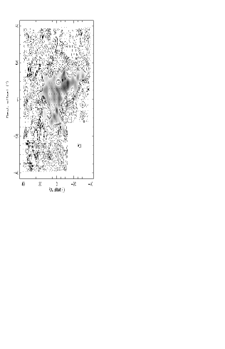
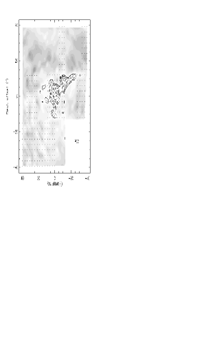
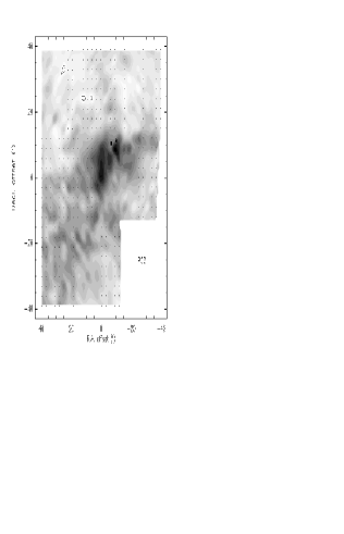
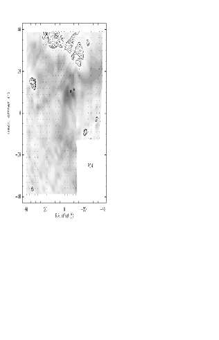
Figure 21: Eigenimages of the four first principal components calculated from the ¹²CO(1–0) data. Negative contours are dashed (contour spacing 0.1), greyscale represents positive values (for PC1 contour spacing is 0.05 else it is 0.2) and the full line is the zero level isocontour

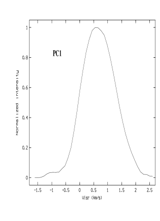
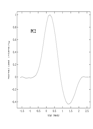
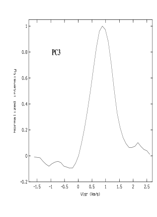
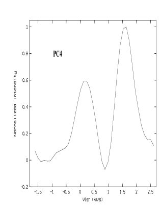
Figure 22: Eigenvectors used to generate the eigenimages shown in Fig. 21

From ¹²CO(1–0) data a 648$\times$40 matrix was constructed containing 648 observed spectra with 40 velocity channels. The velocity range is [-1.6,+2.6] km s^-1 with a channel width of 0.1 km s^-1. Before PCA analysis, the data are standardised, i.e. each spectrum is mean-centred and normalised with its standard deviation.

Figures 21 and 22 show our results. The principal components 1-4 account for 71%, 13%, 7% and 3% of the total variance, respectively. Together, these represent 95% of the total variance in our data. The remaining components are mostly pure noise and are discarded. The importance of the first component shows that the spectra are not independent from each other. As expected, there is a rather continuous variation of line morphology throughout the cloud.

The first principal component, PC1, represents the average spectral profile and the associated map shows the clumpy distribution of the main cloud. The emission corresponds to the structures seen in channel maps at $\sim$0.5 km s^-1. The first eigenvector is roughly gaussian, with position $\sim$0.6 km s^-1 and width 1.4 km ${\rm s}^{-1}$. The following PCs describe successive corrections to the first approximation given by PC1. Looking at the profiles, PC2 suggests a shift in velocity and PC4 a change in the linewidth. PC3 indicates either a small change in the radial velocity or, more likely, the presence of some narrower spectra.

PC2 mainly indicates velocity variations inside central region of L1642 and separates this from the northern part of the field. The eigenvector indicates that these sub-structures are around 0.2 km s^-1 while the northern part has a mean velocity of 1.2 km s^-1. PC3 indicates a region of emission around (0$\arcmin$, 0$\arcmin$) and (-9$\arcmin$, +8.5$\arcmin$) with a velocity around 0.8 km s^-1. Finally, PC4 shows substructures in the core at velocity $\sim$0.1 km s^-1 especially around (-2.5$\arcmin$, +9$\arcmin$), (-8, +17$\arcmin$) and (-8.5$\arcmin$, +9$\arcmin$). The map of PC4 resembles the channel maps between 1.5 and 1.8 km s^-1. The northern part appears patchy, but it is difficult to say if the structure is caused by real clumps or is simply due to noise fluctuations.

The PCA analysis follows a hierarchical scheme: first, it shows the central part of L1642 (0.6 km s^-1), secondly, it discriminates this from the northern part (1.2 km s^-1). Next it reveals additional velocity structure inside L1642 itself (0.2, 0.8 km s^-1), and finally fainter emission at more positive velocity in the extreme north ($\sim$1.5 km s^-1).

A.3 Comparison of the analysis methods

Channel maps are the standard method for analysing kinematic information of molecular line maps. The presentation is mostly limited by the noise. If the channel width is kept constant, the noise will dominate in the line wings. If, on the other hand, noise is suppressed by integration over larger velocity intervals, one loses all information of smaller velocity structures. Furthermore, the signal level varies significantly over the map, and the selection of integration intervals and contour levels is necessarily a compromise. However, one can visually recognise continuous regions of emission even when noise is quite significant. Channel maps do not provide direct information on the spectral profiles because each channel is treated completely separately. This information is obtained indirectly by looking at the maps of consecutive velocity channels.

Both PCA and PMF present the observations as a linear combination of basic spectral components which are extracted from the data. The methods carry out a global fit, and can therefore discern features that are too weak to be detected in any individual spectrum but which are repeated in many observations. When the intensities of the spectral components are determined for a given spectrum, the fit is done using all the relevant channels. The methods are therefore most useful in the case of spectra with low signal-to-noise ratios. The spectral features cannot, of course, be separated unless their relative intensities change over the map. PCA and PMF decompositions compress the information contained in the observation matrix to be presented with just a few components. The result should therefore be easier to interpret. In the case of PCA, however, this is complicated by negative values present both in the profiles and in the component maps.

In the case of our L1642 observations, the three methods agree in the main features. Comparison of the different methods shows that the PMF method is especially able to produce a presentation that is at the same time compact and easy to interpret. For example, a PMF decomposition with $r$=4 reproduces practically all of the structure visible in the very complex channel maps of ¹²CO. Because of the lower signal-to-noise ratio, only three components could be detected in the C¹⁸O data. When the rank of the factorization is lower than the rank of the observation matrix, the presentation is not exact. However, if $r$ is sufficiently large, the fit residuals mostly consist of noise. The study of residuals of the PCA or PMF fits is a very powerful tool for finding deviating spectra (see Sect 3.1). Residuals identify abnormal spectra and show how their profiles differ from the average behaviour.

In channel maps, one has the tendency to interpret intensity variations of separate components as continuous velocity gradients. PMF and PCA explicitly assume that the emission is the sum of components at fixed radial velocities. Velocity gradients are approximated as the sum of two or more spectral components at different velocities, and with gradual changes in the weights of the components. In the northern part of L1642, the channel maps of ¹²CO $J$=1–0 and $J$=2–1 suggest a small velocity gradient towards the north. PMF decomposition with $r$=4 presents the northern part with just one velocity component. With $r$=5, the emission is divided into two components, suggesting the presence of a velocity gradient. With higher $r$, the emission is not divided any further. Within the noise limits the observations are, therefore, consistent with both a small velocity gradient and the presence of two separate emission components.

Appendix B Three-dimensional radiative transfer model

B.1 Mass estimates

The ¹³CO $J$=1–0 and $J$=2–1 observations of L1642 were modelled with a fully three-dimensional model that consisted of 46³ cells arranged on a Cartesian grid. Along two dimensions, the column density distribution follows the distribution obtained from the LTE calculations, and this fixes the size of the model. Along the third dimension (i.e. along the line-of-sight), the density distribution is assumed to be gaussian, with the extent of the cloud similar along the line-of-sight as in the plane of the sky. In the model, the linewidths are caused in roughly equal parts by microturbulence within cells and macroscopic turbulence between cells. The mean velocity of cells on each line-of-sight was shifted according to the velocity of the observed ¹³CO(1–0) line. This enables direct comparison with the observed spectra, but also creates velocity gradients that have a small effect on the excitation. The density distribution was modified according to a volume filling factor, $f$, by reducing the density by two orders of magnitude in a randomly selected fraction 1-$f$ of the cells. This is only a crude approximation of the true cloud structure, but such a model has already been shown to reproduce some of the effects caused by density inhomogeneities (see e.g. Park, Hong, & Minh park96 (1996); Juvela juvela97 (1997)). The three-dimensional model is fundamentally different from the one-dimensional models discussed in Sect. 5, and the comparison of the results should give a good idea of the overall uncertainty of the mass estimates.

The parameter $f$ was varied between 0.1 and 1.0, and model calculations were carried out for $T_{\rm kin}$=8-14 K. The best fit with observations was obtained with $T_{\rm kin}$=8 K, $f=$0.4 and peak density of 1.7$\times 10^{4}$ cm^-3. The total mass of the model cloud was 70 $M_{\sun}$, very similar to the values obtained with spherically symmetric models. The $\chi^{2}$-value of the fit was less than 10% higher at 12 K suggesting that the temperature is not well constrained. Since the cloud size was fixed, the mass decreases when the assumed temperature increases: for $T_{\rm kin}$=14 K it is 37 $M_{\sun}$. The volume filling factor of the best fitting models increases with temperature, and was already 1.0 at 14 K. The $f$-parameter had surprisingly little effect on the results, particularly at higher temperatures. However, because of the macroturbulence, all models contained equal amount of inhomogeneity in the velocity space.

B.2 Comparison of true and LTE column densities

In order to further investigate the errors introduced by the LTE assumption, we computed LTE column density estimates based on 3D cloud models with $T_{\rm kin}$=10 K and volume filling factors $f$=1.0 and $f$=0.1. The model parameters were adjusted so that the model approximately reproduced the ¹³CO observations of L1642. Spectra were calculated for the ¹²CO(1–0) and ¹³CO(1–0) lines, and LTE analysis of the line ratios of the calculated lines resulted in average excitation temperatures of $T_{\rm ex}=$8.9 K for the model with $f$=1.0 and $T_{\rm ex}=$8.4 K for the model with $f$=0.1. LTE column densities were computed based on these average excitation temperatures and the calculated ¹³CO(1–0) spectra. In Fig. 23, the LTE column densities are plotted against the known, true column densities in the models.

For column densities derived from the ¹³CO(1–0) line, the LTE calculations are quite accurate. In the case of $f$=0.1, the scatter is larger because of the inhomogeneity of the cloud, and at high column densities the LTE-estimates may be slightly biased towards low values. The LTE estimate is not very sensitive to the assumed excitation temperature, and even a change of 2 K in the value of $T_{\rm ex}$ has little effect on the derived values. The volume-averaged, true excitation temperatures obtained from the radiative transfer models are close to 5 K, i.e. clearly below the LTE estimates of 8–9 K. However, the large difference is mostly caused by low-density gas at the edges of the cloud, and the bulk of emission comes from denser regions which are much closer to thermalization.

We also plot in Fig. 23 LTE estimates of the column density derived from the model-calculated $J=$2–1 lines, assuming excitation temperatures that are 1 K lower than for the $J=$1–0 line. The column density values are seen to be too low by up to a factor of two. In the case of $f$=0.1, the density of the remaining clumps is higher, and since the gas is closer to thermalization, the LTE estimates are also closer to the true column density values. The results are more sensitive to the value of $T_{\rm ex}$ than in the case of the $J=$1–0 line. The column density values increase if one assumes a lower excitation temperature. However, the LTE estimates of the excitation temperature are less than 1 K lower than for the $J=$1–0 transition, and the same applies to the average excitation temperature in the numerical models. The results show that the column density estimates based on the $J=$2–1 transition are inherently more uncertain than those derived from the $J=$1–0 observations.

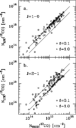
Figure 23: Comparison of LTE column density estimates and the true, beam averaged column densities in three-dimensional model clouds with $T_{\rm kin}$=10 K and volume filling factors 1.0 and 0.1. The lines indicate relations 1.0$\times N_{\rm TRUE}$ and 0.5$\times N_{\rm TRUE}$

References

- (1) Ábrahám P., Balázs L.G., Kun M. 2000, A&A 354, 645
- (2) Bacmann A., André P., Puget J.L., et al. 2000, A&A 361, 555
- (3) Blitz L., Fich M. 1983, in Kinematics, dynamics and structure of the Milky Way, Dordrecht, D. Reidel Publishing Co., page 143.
- (4) Booth R.S., Delgado G., Hagström, M., et al. 1989, A&A 216, 315
- (5) Brown A.G. Hartmann D., Burton W.B. 1995, A&A 300,903
- (6) Falgarone E., Puget J.-L., Perault M. 1992, A&A 257, 715
- (7) Falgarone E., Phillips T.G., Walker C.K. 1991, A&A 378, 186
- (8) Falgarone E., Puget J.-L., 1988, in Galactic and Extragalactic Star Formation, eds. R.E. Pudritz, M. Fich, Kluwer, Dordrecht, P. 195
- (9) Guelin M., Cernicharo J., 1988, in Molecular Clouds in the Milky Way and external galaxies, Springer-Verlag
- (10) Hearty T., Fernández M., Alcalá J.M., Covino E., Neuhäuser R. 2000, A&A 357, 681
- (11) Heiles C., Haffner M., Reynolds R., 1999, ASP conf. Series 168, 211
- (12) Heyer M.H., Schloerb F.P. 1997, ApJ 475, 173
- (13) Ingalls J., Bania T., Lane A., et al., 2000, ApJ 535, 211
- (14) Juvela M. 1997, A&A 322, 943
- (15) Juvela M., Lehtinen K., Paatero P. 1996, MNRAS 280, 616
- (16) Kuntz K.D., Snowden S.L., Verter F. 1997, ApJ 484, 245
- (17) Langer W.D., Wilson R.W., Goldsmith P.F., Beichman C.A., 1989, ApJ 337, 355
- (18) Laureijs R.J., Mattila K., Schnur G. 1987,A&A 184, 269
- (19) Liljeström T., Mattila K. 1988, A&A 196, 243
- (20) Liljeström T., Mattila K., Friberg P. 1989, A&A 210, 337
- (21) Liljeström T. 1991, A&A 244,483
- (22) Murtagh F., Heck A., 1987, Multivariate Data Analysis. Ap. Sp. Sc. Lib., Dordrecht: Reidel, p. 13
- (23) Paatero P. 1999, Journal of Comp. and Graph. Stat., vol. 8, 854
- (24) Padoan P., Juvela M., Bally J., Nordlund Å2000, ApJ 529, 259
- (25) Park Y.S., Hong S.S., Minh Y.C. 1996, A&A 312, 981
- (26) Reipurth B., Heathcote S. 1990, A&A 229, 527
- (27) Reynolds R.J., Odgen P.M. 1979, ApJ 229, 942
- (28) Sandell G., Reipurth B., Gahm G. 1987, A&A 181, 283
- (29) Sfeir D.M., Lallement R., Crifo F., Welsh B.Y. 1999, A&A 346, 785
- (30) Taylor M., Taylor K., Vaile R., 1982, Proc. ASA 4, 440
- (31) Ulich B.L., Haas R.W. 1976, ApJS 30, 247
- (32) Ungerechts H., Bergin E.A., Goldsmith P.F., et al. 1997, ApJ 482, 245
- (33) Ward-Thompson D., Scoot P.F., Hills R.E., André P. 1994, MNRAS 268, 276
- (34) Ward-Thompson D., Motte F., André P. 1999, MNRAS 305, 143