Local and Global Variations of The Fine Structure Constant

Abstract

Using the BSBM varying-alpha theory, with dark matter dominated by magnetic energy, and the spherical collapse model for cosmological structure formation, we have studied the effects of the dark-energy equation of state and the coupling of alpha to the matter fields on the space and time evolution of alpha. We have compared its evolution inside virialised overdensities with that in the cosmological background, using the standard ($\Lambda=0$) $CDM$ model of structure formation and the dark-energy modification, $wCDM$. We find that, independently of the model of structure formation one considers, there is always a difference between the value of alpha in an overdensity and in the background. In a $SCDM$ model, this difference is the same, independent of the virialisation redshift of the overdense region. In the case of a $wCDM$ model, especially at low redshifts, the difference depends on the time when virialisation occurs and the equation of state of the dark energy. At high redshifts, when the $wCDM$ model becomes asymptotically equivalent to the $SCDM$ one, the difference is constant. At low redshifts, when dark energy starts to dominate the cosmological expansion, the difference between alpha in a cluster and in the background grows. The inclusion of the effects of inhomogeneity leads naturally to no observable local time variations of alpha on Earth and in our Galaxy even though time variations can be significant on quasar scales. The inclusion of the effects of inhomogeneous cosmological evolution are necessary if terrestrial and solar-system bounds on the time variation of the fine structure ’constant’ are to be correctly compared with extragalactic data.

1 Introduction

Studies of the time and spatial variations of the fine structure ’constant’, $\alpha$, are motivated primarily by recent observations of small variations in relativistic atomic structure in quasar absorption spectra (Murphy et al., 2001, 2003; Webb et al., 2001, 1999). Three data sets, containing observations of the spectra of 128 quasars continue to suggest that the fine structure ’constant’, was smaller at redshifts $z=0.2-4.2$ than the current terrestrial value $\alpha_{0}=7.29735308\times 10^{-3}$, with $\Delta\alpha/\alpha\equiv\{\alpha(z)-\alpha_{0}\}/\alpha_{0}=-0.57\pm 0.11\times 10^{-5}$ (Murphy, Flambaum & Webb, 2003). If this interpretation of these observations proves correct then there are important consequences for our understanding of the forces of nature at low energies as well as for the question of the links between couplings in higher dimensions and the three-dimensional shadows that we observe (Barrow, 2002) . Any slow change in the scale of the extra-dimensions would be revealed by measurable changes in our four-dimensional “constants”. Further observational tests may help to provide independent tests of the quasar data (Darling, 2003). Attempts to generalise the standard model by including scalar fields which carry the space-time variation of the fine structure ’constant’ could have important connections with the dark energy that is currently accelerating the expansion of the universe (Parkinson, Bassett, & Barrow, 2003; Wetterich, 2003) and also create potentially detectable violations of the weak equivalence principle (Dvali & Zaldarriaga, 2002; Olive & Pospelov, 2002; Damour & Polyakov, 1994; Nordtvedt, 2002).

Several theories have been proposed to investigate the implications of a varying fine structure ’constant’. Some based on grand unification theories (Langacker, Segre & Strassler, 2002; Dent & Fairbairn, 2003; Fritzsch, 2002; Calmet & Fritzsch, 2002a, b; Marciano, 1984; Banks, Dine & Douglas, 2002; Armendariz-Picon, 2002), some with extra-dimensions (Brax et al., 2003; Palma et al., 2003; Youm, 2002; Dent, 2003; Paccetti Correia , Schmidt & Tavartkiladze, 2002), others in four dimensions (Bekenstein, 1982, 2003; Barrow, Sandvik & Magueijo, 2002a, b; Barrow, Magueijo & Sandvik, 2002b; Sandvik, Barrow & Magueijo, 2002; Barrow & Mota, 2002; Huang & Li, 2002; Kostelecky, Lehnert & Perry, 2002) and even in two dimensional black holes (Vagenas, 2003). All these models need to satisfy the present constraints on the variations in $\alpha$. These constraints can be divided into two main groups: local and astro-cosmological. The local constraints derive from experiments in our local bound gravitational system: the Oklo natural reactor $(z=0.14)$, where $\left|\frac{\Delta\alpha}{\alpha}\right|\leq 10^{-7}$ (Fujii et al, 2000; Damour & Dyson, 1996; Fujii, 2003; Shlyakhter, 2003). However, the use of an equilibrium neutron spectrum in this analyses has recently been criticised by (Lamoreaux, 2003). More realistic modelling leads to a best fit of the data to non-zero shift $\Delta\alpha/\alpha=4.5\times 10^{-8}$. ; the intra solar-system decay rate ${}^{187}\mathrm{Re}~{}\rightarrow~{}^{187}\mathrm{Os}$, $(z=0.45)$, where $\left|\frac{\Delta\alpha}{\alpha}\right|\leq 10^{-7}$ (Olive et al., 2002; Fujii & Iwanoto, 2003; Olive et al., 2003); and the stability of terrestrial atomic clocks $(z=0)$, where $\left|\frac{\dot{\alpha}}{\alpha}\right|<4.2\times 10^{-15}~{}\mathrm{yr}^{-1}$ (Marion et al., 2002). Other limits arise from weak equivalence experiments (Dvali & Zaldarriaga, 2002; Olive & Pospelov, 2002; Damour & Polyakov, 1994; Nordtvedt, 2002; Magueijo, Barrow & Sandvik, 2002) but the limits they provide are more model dependent. In addition to the the above-mentioned positive signal from quasar absorption spectra, the astro-cosmological constraints are: the cosmic microwave background radiation $(z=10^{3})$, where $\left|\frac{\Delta\alpha}{\alpha}\right|<10^{-2}$ (Martins et al., 2003; Avelino et al., 2000; Battye, Crittenden & Weller, 2001; Hannestad, 1999; Kaplinghat, Scherrer & Turner, 1999) and Big Bang nucleosynthesis $(z=10^{8}-10^{10})$, where $\left|\frac{\Delta\alpha}{\alpha}\right|\leq 2\times 10^{-2}$ (Martins et al., 2003; Avelino et al., 2000; Battye, Crittenden & Weller, 2001). Other emission-line studies (Bahcall, Steinhardt, & D.Schlegel, 2003) give weak bounds of $\frac{\Delta\alpha}{\alpha}\leq-2\pm 1.2\times 10^{-4}$ which are comparable to the earlier limits of refs. (Cowie & Songaila, 1995; Ivanchik, Potekhin & Varshalovich, 1999; Levshakov, 1994).

There is a potential discrepancy between local and astro-cosmological constraints; in particular, between the constraint of $\Delta\alpha/\alpha\leq 10^{-7}$ at redshift $0\leq z\leq 0.45$, coming from the $\beta$-decay in meteoritic samples (Olive et al., 2002, 2003), and the explicit variation in $\alpha$ of $\Delta\alpha/\alpha\approx 10^{-6}$ at $0.2\leq z\leq 4.2$, coming from the low-redshift end of the quasar absorption spectra (Murphy, Webb & Flambaum, 2003; Murphy et al., 2001, 2003; Webb et al., 2001, 1999). A successful theory of varying $\alpha$ needs to explain this difference. This is a challenge. Models which use a very light scalar field, to drive variations in $\alpha$, need an extreme fine tuning in order to satisfy the phenomenological constraints coming from geochemical data (Oklo, $\beta$-decay), the present equivalent principle tests, and the quasar absorption spectra, simultaneously (Damour, 2003). The presence of the dark energy plays an important role in any potential reconciliation because in simple scalar theories (Sandvik, Barrow & Magueijo, 2002) any variation of $\alpha$ turns off as the universe starts to accelerate.

A solution to this problem was proposed by us in (Mota & Barrow, 2003), where numerical simulations were shown to display behaviour for the evolution of $\alpha$ inside an overdensity that differs from that in the background universe, during the formation of non-linear large-scale structures. All previous studies of the variation of ’constants’ in cosmology had neglected the effects of inhomogeneity in the Universe and the fact that our local observational constraints on varying constants are made within non-expanding matter overdensities. We found that the fine structure ’constant’ evolves differently inside virialised clusters compared to the background universe. Specifically, $\alpha$ becomes a effectively time-independent inside a gravitationally bound overdensity after its virialisation. The fact that local $\alpha$ values ’freeze in’ at virialisation, means we would observe no time variations in $\alpha$ on Earth, or elsewhere in our Galaxy, even though time-variations in $\alpha$ might still be occurring on extragalactic scales at a detectable level. For a typical galaxy cluster, the value of $\alpha$ today will be the value of $\alpha$ at the virialisation time of the cluster. Hence, the local constraints on time variations in the fine structure ’constant’, can easily give a value that is $10-100$ times smaller than is inferred on extra-galactic scales from quasar absorption spectra.

The reason why the growth and gravitational binding of matter inhomogeneities affects the evolution of $\alpha$ is simple. Any varying-$\alpha$ theory implies the existence of a scalar field carrying the variations in $\alpha$. This field is coupled to some selection of the matter fields, depending upon their interactions (Parkinson, Bassett, & Barrow, 2003; Anchordoqui & Goldberg, 2003; Wetterich, 2003). Due to this coupling, any inhomogeneities of the latter will then affect the evolution of $\alpha$. This effect is not only important in the non-linear regime of large-scale structure formation (Barrow & O’Toole, 1999). Even in the linear regime of cosmological perturbations, when these are small, $\frac{\delta\alpha}{\alpha}$ grows and tracks $\frac{\delta\rho_{m}}{\rho_{m}}\propto t^{2/3}$ during the dust-dominated era on scales smaller than the Hubble radius (Barrow & Mota, 2003). It is therefore important to study the cosmological evolution of the fine structure ’constant’ taking into account a more realistic universe, where matter inhomogeneities grow and lead to the formation of bounded objects.

The dependence of the fine structure constant on the density of the matter fields leads to spatial variations of $\alpha$. Spatial variations imply the existence of ’fifth force’ effects. The fifth force induces an anomalous acceleration which depends on the material composition of the test particle, and so violates the weak equivalence principle (WEP). This is a general feature of any varying-$\alpha$ theory but he magnitude of the WEP violations is model dependent. In the case of the Bekenstein-Sandvik-Barrow-Magueijo (BSBM) model, such violations are within the current WEP experiments (Barrow, Magueijo & Sandvik, 2002a). In particular, it was shown in (Magueijo, Barrow & Sandvik, 2002) that spatial variations of $\alpha$ in the vicinity of compact massive objects may well be within an order of magnitude below the existing experimental bounds (see appendix B).

There are two main features which affect the evolution of the fine structure ’constant’ in a universe where large scale structures are formed. The most obvious, is the coupling between the scalar field, which drives variations in $\alpha$, and the matter fields. The second is the dependence of non-linear models of structure formation on the equation of state of the universe, and in particular that of the dark energy (Lahav et al., 1991; Wang & Steinhardt, 1998). In this paper we will study the dependence of $\alpha$ on these two quantities in the BSBM varying-$\alpha$ model. In this theory, variations in $\alpha$ are driven by the electromagnetically-coupled matter fields and the effects of inhomogeneity are large. In the next section we briefly summarise the BSBM model (Sandvik, Barrow & Magueijo, 2002) and the spherical collapse model for the development of non-linear cosmological inhomogeneities. In section three, we investigate the dependence of the fine structure ’constant’ on the equation of state of the dark energy. In section four, we show how spatial variations in $\alpha$ may occur due to possible spatial variations in the coupling of $\alpha$ to the matter fields. We summarise our conclusions in section five.

2 The BSBM Theory and the Spherical-Infall Model

2.1 The Background

We will study space-time variations of $\alpha$ in the BSBM theory (Sandvik, Barrow & Magueijo, 2002), which assumes that the total action is given by:

$$S=\int d^{4}x\sqrt{-g}\left(\mathcal{L}_{g}+\mathcal{L}_{matter}+\mathcal{L}_{\psi}+\mathcal{L}_{em}e^{-2\psi}\right)$$ (1)

In this varying-$\alpha$ theory, the quantities $c$ and $\hbar$ are taken to be constant, while $e$ varies as a function of a real scalar field $\psi(x^{\beta}),$ with $e=e_{0}e^{\psi}$, $\mathcal{L}_{\psi}={\frac{\omega}{2}}\partial_{\mu}\psi\partial^{\mu}\psi$, $\omega$ is a coupling constant, and $\mathcal{L}_{em}=-\frac{1}{4}f_{\mu\nu}f^{\mu\nu}$; $\mathcal{L}_{matter}$ is the Lagrangian of the matter fields. The gravitational Lagrangian is as usual $\mathcal{L}_{g}=-\frac{1}{16\pi G}R$, with $R$ the Ricci curvature scalar, and we have defined an auxiliary gauge potential by $a_{\mu}=\epsilon A_{\mu}$ and a new Maxwell field tensor by $f_{\mu\nu}=\epsilon F_{\mu\nu}=\partial_{\mu}a_{\nu}-\partial_{\nu}a_{\mu}$, so the covariant derivative takes the usual form, $D_{\mu}=\partial_{\mu}+ie_{0}a_{\mu}$. The fine structure ’constant’ is then given by $\alpha\equiv\alpha_{0}e^{2\psi}$ with $\alpha_{0}$ the present value measured on Earth today.

The background universe will be described by a flat, homogeneous and isotropic Friedmann metric with expansion scale factor $a(t)$. The universe contains pressure-free matter, of density $\rho_{m}$ $\propto a^{-3}$ and a dark-energy fluid with a constant equation of state parameter, $w_{\phi}=p_{\phi}/\rho_{\phi}$, and an energy-density $\rho_{\phi}\propto a^{-3(1+w_{\phi})}$. In the case where dark energy is the cosmological constant $\Lambda$, $\rho_{\phi}\equiv\rho_{\Lambda}\equiv$ $\Lambda/(8\pi G)$ and $w_{\phi}=-1$. Varying the total Lagrangian, we obtain the Friedmann equation ($\hbar=c\equiv 1$):

$$H^{2}=\frac{8\pi G}{3}\left(\rho_{m}\left(1+\left|\zeta\right|e^{-2\psi}\right)\ +\rho_{\psi}+\rho_{\phi}\right),$$ (2)

where $H\equiv\dot{a}/a$ is the Hubble rate, $\rho_{\psi}=\frac{\omega}{2}\dot{\psi}^{2},$ and $\zeta=\mathcal{L}_{em}/\rho_{m}$ is the fraction of the matter which carries electric or magnetic charges. The value (and sign) of $\zeta$ for baryonic and dark matter has been disputed (Dvali & Zaldarriaga, 2002; Olive et al., 2002; Sandvik, Barrow & Magueijo, 2002). It is the difference between the percentage of mass in electrostatic and magnetostatic forms. As explained in (Sandvik, Barrow & Magueijo, 2002), we can at most estimate this quantity for neutrons and protons, with $\zeta_{n}\approx\zeta_{p}\sim 10^{-4}$. We may expect that for baryonic matter $\zeta\sim 10^{-4}$, with composition-dependent variations of the same order. The value of $\zeta$ for the dark matter, for all we know, could be anything between -1 and 1. Superconducting cosmic strings, or magnetic monopoles, display a negative $\zeta$, unlike more conventional dark matter. It is clear that the only way to obtain a cosmologically increasing $\alpha$ in BSBM is with $\zeta<0$, i.e with unusual dark matter, in which magnetic energy dominates over electrostatic energy.

The term $\left|\zeta\right|e^{-2\psi}$ represents an average of the (always positive) energy density contribution from the non-relativistic matter which interacts electromagnetically.

The scalar-field evolution equation is

$$\ddot{\psi}+3H\dot{\psi}=-\frac{2}{\omega}\ e^{{-2\psi}}\zeta\rho_{m}.$$ (3)

In this article, we consider that the scalar field responsible for the variations of $\alpha$ is coupled to dark matter and to baryons. Both species are included in the $\zeta\rho_{m}$ terms. The coupling to dark matter appears in general in any dilaton type theory, like string theory, where a scalar field is coupled to all the terms in the Lagrangian, but not necessarily in the same way. In the case of BSBM models, the coupling is motivated by certain classes of dark-matter models and their supersymmetric versions Olive & Pospelov (2002). The coupling between $\alpha$ and dark-matter could permit dark-matter-photon interactions of which would be mediated by the scalar field. Due to the “invisible” nature of dark matter, its coupling to $\alpha$ is tightly constrained. In the case of BSBM models several constraints were imposed on $\zeta$ in (Olive & Pospelov, 2002). Other motivations and consequences of this coupling are investigated in Boehm et al. (2002), where dark-matter-photon interactions are constrained using the CMBR anisotropies and the matter power spectrum. In Boehm et al. (2002) the cross section associated to the dark-matter - photon interaction is constraint to be $\sigma_{\gamma-DM}/m_{DM}\leq 10^{-6}\sigma_{th}/(100\,GeV)\approx 6\times 10^{-33}cm^{2}\,GeV^{-1}$, where $\sigma_{\gamma-DM}$ is the dark-matter-photon cross section, $m_{DM}$ is the dark-matter particle mass and $\sigma_{th}$ is the Thomson cross section. Since in our case $\sigma_{th}\sim\alpha^{2}\sim\alpha_{0}^{2}e^{4\psi}$, then an approximate constraint to the coupling between the scalar field and dark-mater can be set imposing that $\sigma_{\psi-DM}\sigma_{\psi-\gamma}\leq\sigma_{\gamma-DM}$, where $\sigma_{\psi-DM}\sim\zeta^{2}e^{-4\psi}/\omega^{2}$ and $\sigma_{\psi-\gamma}\sim e^{-4\psi}$. Roughly giving $|\zeta|\leq 10^{-3}\alpha_{0}\sim 10^{-6}$, when assuming the “usual” $m_{DM}\sim 100\,GeV$. In this article we will use $|\zeta|\sim 10^{-8}$ as a reference value. In reality, as we show in section 4, the cosmological evolution of the fine structure constant is independent of value of $|\zeta|$ due to a degeneracy between the initial condition for $\psi$ and the coupling to the matter fields. The independence of our results with respect to the value of $\zeta/\omega$ give us the freedom to make the coupling to dark matter as small as desired. For instance, we are free to make the cross section photon - scalar field - dark matter smaller enough to satisfy all the constraints coming from the “invisible” nature of dark-matter. In a similar way, we are free to constraint the value of $\zeta/\omega$ in order to avoid problems associated with the so called self-interacting dark matter, which could radiate and cool, due to its ’magnetic’ nature. All these features could be combined to constraint the value of $\zeta$. However that would be a lengthy and a highly model-dependent analysis, and will be considered by the authors elsewhere.

2.2 The Density Inhomogeneities

In order to study the behaviour of the fine structure ’constant’ inside overdensities we will use the spherical-infall model (Padmanabhan, 1995). This will describe how the field in the overdensity breaks away from the field in background expansion. The overdense sphere behaves like a spatially closed sub-universe. The density perturbations need not to be uniform within the sphere: any spherically symmetric perturbation will evolve within a given radius in the same way as a uniform sphere containing the same amount of mass. Similar results could be obtained by performing the analysis of the BSBM theory using a spherically symmetric Tolman-Bondi metric for the background universe with account taken for the existence of the pressure contributed by the dark energy and the $\psi$ field. In what follows, therefore, density refers to mean density inside a given sphere.

Consider a spherical perturbation with constant internal density which, at an initial time, has an amplitude $\delta_{i}>0$ and $|\delta_{i}|\ll 1$. At early times the sphere expands along with the background. For a sufficiently large $\delta_{i},$ gravity prevents the sphere from expanding. Three characteristic phases can then be identified. Turnaround: the sphere breaks away from the general expansion and reaches a maximum radius. Collapse: if only gravity is significant, the sphere will then collapse towards a central singularity where the densities of the matter fields would formally go to infinity. In practice, pressure and dissipative physics intervene well before this singularity is reached and convert the kinetic energy of collapse into random motions. Virialisation: dynamical equilibrium is reached and the system becomes stationary: there are no more time variations in the radius of the system, $R$, or in its energy components. This phase determines the final pattern of variations in $\alpha,$ which becomes a constant inside the virialised region, otherwise the system would be unable to virialise (Mota & Barrow, 2003). Meanwhile, depending upon the equation of state of the dominant matter field, $\alpha$ can continue to change in the cosmological background. This behaviour naturally creates a situation where time variation of $\alpha$ on large cosmological scales is accompanied by unchanging behaviour locally within galaxies and our solar system. It would explain the apparent discrepancy between the results of the quasars absorption spectra observations and the $\beta$-decay rate deductions from meteorite data (Olive et al., 2002).

The evolution of a spherical overdense patch of scale radius $R(t)$ is given by the Friedmann acceleration equation:

$$\frac{\ddot{R}}{R}=-\frac{4\pi G}{3}\left(\rho_{cdm}\left(1+\left|\zeta\right|e^{-2\psi_{c}}\right)+4\rho_{\psi_{c}}+(1+3w_{\phi_{c}})\rho_{\phi_{c}}\right),$$ (4)

where $\rho_{cdm}$ is the density of cold dark matter in the cluster, $\rho_{\phi_{c}}$ is the energy density of the dark energy inside the cluster and $\rho_{\psi_{c}}\equiv\frac{\omega}{2}\dot{\psi}_{c}^{2}$, where $\psi_{c}$ represents the scalar field inside the overdensity. We have also used the equations of state $p_{\psi_{c}}=\rho_{\psi_{c}}$, $p_{cdm}=0$ and $p_{\phi_{c}}=w_{\phi_{c}}\rho_{\phi_{c}}$.

In the cluster, the evolutions of $\psi_{c}$, $\rho_{cdm}$ and $\rho_{\phi_{c}}$ are given by

$$\ddot{\psi_{c}}+3\frac{\dot{R}}{R}\dot{\psi_{c}} = -\frac{2}{\omega}e^{-2\psi_{c}}\zeta\rho_{cdm},$$ (5)

$$\dot{\rho}_{cdm} = -3\frac{\dot{R}}{R}\rho_{cdm},$$ (6)

$$\dot{\rho}_{\phi_{c}} = -3\frac{\dot{R}}{R}\left(1+w_{\phi_{c}}\right)\rho_{\phi_{c}}.$$ (7)

We will evolve the spherical overdensity from high redshift until its virialisation occurs. According to the virial theorem, equilibrium will be reached when $T=\frac{1}{2}R\frac{\partial U}{\partial R}$; $T$, is the average total kinetic energy, and $U$ is the average total potential energy in the sphere. Note that we obtain the usual $T=\frac{n}{2}U$ condition, for any potential with a power-law form ($U\propto R^{n}$), which includes our case. It is useful to write the condition for virialisation to occur in terms of the potential energies associated the different components of the overdensity. The potential energy for a given component ${}^{\prime}x^{\prime}$ can be calculated from its general form in a spherical region (Landau & Lifshitz, 1975):

$$U_{x} = 2\pi\int_{0}^{R}\rho_{tot}\phi_{x}r^{2}dr,$$ (8)

$$\phi_{x}\left(r\right) = -2\pi G\rho_{x}\left(R^{2}-\frac{r^{2}}{3}\right),$$ (9)

where $\rho_{tot}$ is the total energy density inside the sphere, $\phi_{x}$ is the gravitational potential due to the $\rho_{x}$ density component.

In the case of a $\Lambda CDM$ model, the potential energies inside the cluster are:

$$U_{G} = -\frac{3}{5}GM^{2}R^{-1},$$ (10)

$$U_{\Lambda} = -\frac{4}{5}\pi G\rho_{\Lambda}MR^{2},$$ (11)

$$U_{\psi_{c}} = -\frac{3}{5}GMM_{\psi_{c}}R^{-4},$$ (12)

where $U_{G}$ is the potential energy associated with the uniform spherical overdensity, $U_{\Lambda}$ is the potential associated with $\Lambda,$ and $U_{\psi_{c}}$ is the potential associated with $\psi_{c}.$ $M=M_{cdm}+M_{\psi_{c}}$ is the cluster mass, with

$$M_{cdm} = \frac{4\pi}{3}\rho_{cdm}(1+|\zeta|e^{-2\psi_{c}})R^{3},$$ (13)

$$M_{\psi_{c}} = \frac{4\pi}{3}\rho_{\psi_{c}}R^{6}.$$ (14)

The virial theorem will be satisfied when

$$T_{vir}=-\frac{1}{2}U_{G}+U_{\Lambda}-2U_{\psi_{c}},$$ (15)

where $T_{vir}$ $=\frac{1}{2}M\bar{v}_{vir}^{2}$ is the total kinetic energy at virialisation and $\bar{v}_{vir}^{2}$ is the mean-square velocity of the components of the cluster.

Using the virial theorem (15) and energy conservation at the turnaround and cluster virialisation times, we obtain an equilibrium condition only in terms of the potential energies:

$$\frac{1}{2}U_{G}(z_{v})+2U_{\Lambda}(z_{v})-U_{\psi_{c}}(z_{v})=U_{G}(z_{ta})+U_{\Lambda}(z_{ta})+U_{\psi_{c}}(z_{ta}),$$ (16)

where $z_{v}$ is the redshift of virialisation and $z_{ta}$ is the redshift at the turnaround of the over-density at its maximum radius, when $R=R_{max}$ and $\dot{R}\equiv 0$. In the case where $\zeta=0$ and $\psi=\dot{\psi}=0$ we reduce to the usual virialisation condition for $\Lambda CDM$ models with no variation of $\alpha$ (Lahav et al., 1991; Wang & Steinhardt, 1998). The generalisation from the cosmological constant case to a dark-energy fluid with a general equation of state $w_{\phi}$ is straightforward. One just needs to note that the potential energy associated to the dark-energy fluid is

$$U_{\phi_{c}}=-\frac{3}{5}GM_{\phi_{c}}MR^{2-3\left(1+w_{\phi_{c}}\right)},$$

where $M_{\phi_{c}}$ is mass associated of that fluid, which is given by

$$M_{\phi_{c}}=\frac{4\pi}{3}\rho_{\phi_{c}}R^{3\left(1+w_{\phi_{c}}\right)}.$$

2.3 Setting the Initial Conditions

The behaviour of the fine structure ’constant’ during the evolution of a cluster can now be obtained numerically by evolving the background Friedmann equations (2) and (3) together with the cluster evolution equations (4)-(7) until the virialisation condition holds. In order to satisfy the constraints imposed by the observations, we need to set up initial conditions for the evolution. Since the Earth is now inside a virialised overdense region, the initial condition for $\psi$ is chosen so as to obtain our measured laboratory value of $\alpha$ at virialisation, $\alpha_{c}(z_{v})\equiv\alpha_{v}=\alpha_{0}$. But, since the redshift at which our cluster has virialised is uncertain, we will choose a representative example where virialisation occurs over the range $0<z_{v}<5$. This is just for illustrative purposes, since in reality, the initial condition for $\psi$ needs to be fixed only once, for our Galaxy. Hence, $\alpha$ in other clusters will have a lower or higher value (with respect to $\alpha_{0}$) depending on their $z_{v}$ values (Mota & Barrow, 2003).

After we have set $z_{v}$ for Earth, another constraint we need to satisfy is given by the quasar observations (Murphy, Webb & Flambaum, 2003). This means that when comparing the value of the fine structure ’constant’ on Earth, at its virialisation, $\alpha_{v}=\alpha_{0}$, with the value of the fine structure ’constant’ of another region at some given redshift in the range accessed by the quasar spectra, $3.5\geq z\geq 0.5$, we need to obtain $\Delta\alpha/\alpha\equiv(\alpha(z)-\alpha_{v})/\alpha_{v}\approx-5.4\times 10^{-6}$. This raises the question as to the location of the clouds where the quasar absorption lines are formed: are they in a region which should be considered as part of the background or in an overdensity with somewhat lower contrast than exists in our Galaxy? Unfortunately, this question cannot be answered because we do not know the density of the clouds, only the column density. Nevertheless, these clouds are much less dense than the solar system. Because of this, it is a very good approximation to assume that the clouds possess the background density.

Thus, the initial conditions for $\psi$ are chosen so as to obtain our measured laboratory value of $\alpha$ at virialisation $\alpha_{c}(z_{v})=\alpha_{0}$ and to match the latest observations (Murphy, Webb & Flambaum, 2003) for background regions at $3.5\geq|z-z_{v}|\geq 0.5$.

Here we may also wonder about possible measurements of $\alpha$ in Lyman-alpha systems and whether similar considerations should be applied because of local variations in density compared to this in the solar system. Assuming that the density of the Lyman-alpha systems are much smaller than the Earth, we would expect to find a difference in $\alpha$ with respect to the value measured on Earth. This difference could even be of the same order as the one found in the quasar spectra. However, this is dependent on the density of the clouds and redshift we are making the measurements. Unfortunately we do not know the local density, only the column density along the line of sight. In order to make some numerical predictions, we would need to create a model populated with clouds of different density but there are too many variables to make a reliable estimate of the effects at present. In the future it may be possible, with the accumulation of very large archives of data, to exploit the known differences in column density in the different types of system where the absorption lines are forms to search for correlations with column density. The damped Lyman-alpha and Lyman-limit systems in the quasar absorption-system data sets have column densities of order or exceeding $2\times 10^{17}cm^{-1}$ and $2\times 10^{20}cm^{-1}$ respectively. Again, rigorous exploitation of any perceived systematic trend in alpha between systems of different column density would require the construction of a HI density model in the vicinity of the absorption system.

3 The Dependence on the Dark-Energy Equation of Sate

Non-linear models of structure formation will present different features depending on the equation of state of the universe (Lahav et al., 1991; Wang & Steinhardt, 1998). The main difference is the way the parameter $\Delta_{c}=\rho_{cdm}(z_{c})/\rho_{b}(z_{v})$ evolves with the redshift. The evolution of $\Delta_{c}$ depends on the equation of state of the dark-energy component which dominates the expansion dynamics. For instance, in a $\Lambda CDM$ model, the density contrast, $\Delta_{c}$ increases as the redshift decreases. At high redshifts, the density contrast at virialisation becomes asymptotically constant in standard ($\Lambda=0$) $CDM$, with $\Delta_{c}\approx 178$ at collapse or $\Delta_{c}\approx 148$ at virialisation. This behaviour is common to other dark-energy models of structure formation ($wCDM$), where the major difference is in the magnitude and the rate of change of $\Delta_{c}$ at low redshifts.

The local value of the fine structure ’constant’ will be a function of the redshift and will be dependent on the density of the region of the universe we measure it, according to whether it is in the background or an overdensity (Mota & Barrow, 2003). The density contrast of the virialised clusters depends on the dark-energy equation of state parameter, $w_{\phi}$ . Hence, the evolution of $\alpha$ will be dependent on $w_{\phi}$ as well.

What difference we would expect to see in $\alpha$ if we compared two bound systems, like two clusters of galaxies? And how does the difference depend on the cosmological model of structure formation? These questions can be answered by looking at the time and spatial variations of $\alpha$ at the time of virialisation. The space variations will be tracked using a ’spatial’ density contrast,

$$\frac{\delta\alpha}{\alpha}\equiv\frac{\alpha_{c}-\alpha_{b}}{\alpha_{b}}$$ (17)

which is computed at virialisation (where $\alpha_{c}(z=z_{v})=\alpha_{v}$). We assume there are no changes after this time.

Since the main dependence of $\alpha$ is on the density of the clusters and the redshift of virialisation, we will only study dark-energy models where $w_{\phi}$ is a constant. Any effect contributed by a time-varying equation of state should be negligible, since the important feature is the average equation of state of the universe. This may not be the case for the models where the scalar field responsible for the variations in $\alpha$ is coupled to dark energy (Parkinson, Bassett, & Barrow, 2003; , 2003; Anchordoqui & Goldberg, 2003).

In order to have a qualitative behaviour of the evolution of the fine structure ’constant’, at the virialisation of an overdensity, we will then compare the standard Cold Dark Matter model, $SCDM$, to the dark-energy Cold Dark Matter, $wCDM$, models. In particular, we will examine the representative cases of $w_{\phi}=-1,-0.8,-0.6$. All models will be normalised to have $\alpha_{v}=\alpha_{0}$ at $z=0$ and to satisfy the quasar observations (Murphy, Webb & Flambaum, 2003), as discussed above. This normalisation, although unrealistic (Earth did not virialise today), give us some indication of the dependence of the time and spatial evolution in $\alpha$ on the different models. In reality, this approximation will not affect the order of magnitude of the spatial and time variations in $\alpha$ for the cases of virialisation at low redshift (Mota & Barrow, 2003).

3.1 Time-shifts and the evolution of $\alpha$

The final value of $\alpha$ inside virialised overdensities and its evolution in the background is shown in Figures 1 and 2, respectively. From these plots, a feature common to all the models stands out: the fine structure ’constant’ in the background regions has a lower value than inside the virialised overdensities. Also, its eventual local value depends on the redshift at which the overdensity virialises.

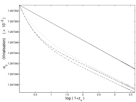
Figure 1: Value of $\alpha$ inside clusters as a function of $\log(1+z_{v})$, the epoch of virialisation. Solid line corresponds to the standard ($\Lambda=0$) $CDM$, dashed line is the $\Lambda CDM$, dashed-dotted corresponds to a $wCDM$ model with $w_{\phi}=-0.8$, dotted-line corresponds to a $wCDM$ model with $w_{\phi}=-0.6$. In all the models, the initial condition were set in order to have $\alpha_{c}(z=0)=\alpha_{0}$ and to satisfy $\Delta\alpha/\alpha\approx-5.4\times 10^{-6}$ at $3.5\geq|z-z_{v}|\geq 0.5$.

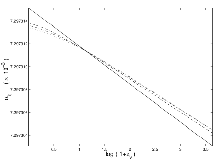
Figure 2: The value of $\alpha$ in the background universe at the epoch of cluster virialisation, $\log(1+z_{v})$. The solid line corresponds to the standard ($\Lambda=0$) $CDM$, dashed line is the $\Lambda CDM$, dashed-dotted line corresponds to a $wCDM$ model with $w_{\phi}=-0.8$, dotted line corresponds to a $wCDM$ model with $w_{\phi}=-0.6$. In all models, the initial condition were set in order to have $\alpha_{c}(z=0)=\alpha_{0}$ and to satisfy $\Delta\alpha/\alpha\approx-5.4\times 10^{-6}$ at $3.5\geq|z-z_{v}|\geq 0.5$.

As expected, the equation of state of the dark energy affects the evolution of $\alpha,$ both in the overdensities and the background. A major difference arises if we compare the $SCDM$ and $wCDM$ models. In a $SCDM$ model, the fine structure ’constant’ is always a growing function, both in the background and inside the overdensities, and the growth rate is almost constant. In a $wCDM$ model, the evolution of $\alpha$ will depend strongly on whether one is inside a cluster or in the background. In the $wCDM$ background, $\alpha_{b}$ becomes constant (independent of the redshift) as the universe enters the phase of accelerated expansion. Inside the clusters, $\alpha_{v}$ will always grow and its value now will depend on the redshift at which virialisation occurred. The cumulative effect of this growth increases as we consider overdensities which virialise at increasingly lower redshift.

These differences arise due to the dependence of the fine structure ’constant’ on the equation of state of the universe and the density of the regions we are measuring it. In a $SCDM$ model, we will always live in a dust-dominated era. The fine structure ’constant’ will then be an ever-increasing logarithmic function of time, $\alpha\propto\ln(t)$ (Sandvik, Barrow & Magueijo, 2002; Barrow & Mota, 2002). The growth rates of $\alpha_{b}$ and $\alpha_{c}$ will be constant, since $\Delta_{c}$ is independent of the redshift in a $SCDM$ model. In a $wCDM$ model, dark energy plays an important role at low redshifts. As we reach low redshifts, where dark energy dominates the universal expansion, $\alpha_{b}$ becomes a constant (Sandvik, Barrow & Magueijo, 2002; Barrow & Mota, 2002), but $\Delta_{c}$ continues to increase, as will $\alpha_{c}$ (Mota & Barrow, 2003). The growth of $\alpha_{v}$ becomes steeper as we go from a dark-energy fluid with $w_{\phi}=-0.6$ to the $\Lambda$-like case of $w_{\phi}=-1$. The intermediate situation is where $w_{\phi}=-0.8$, due to the dependence of $\Delta_{c}$ on $w_{\phi}$.

Similar conclusions can be drawn with respect to the ’time shift’ of the fine structure ’constant’, ($\Delta\alpha/\alpha$), at virialisation, see Figures 3 and 4.

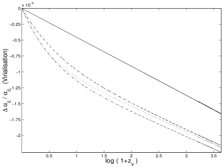
Figure 3: Variation of $\Delta\alpha/\alpha$ inside clusters as a function of the epoch of virialisation, $\log(1+z_{v})$. The solid line corresponds to the standard ($\Lambda=0$) $CDM$, the dashed line is the $\Lambda CDM$, the dashed-dotted line corresponds to a $wCDM$ model with $w_{\phi}=-0.8$, the dotted line corresponds to a $wCDM$ model with $w_{\phi}=-0.6$. In all models, the initial conditions were set in order to have $\alpha_{c}(z=0)=\alpha_{0}$ and to satisfy $\Delta\alpha/\alpha\approx-5.4\times 10^{-6}$ at $3.5\geq|z-z_{v}|\geq 0.5$.

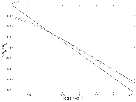
Figure 4: Variation of $\Delta\alpha/\alpha$ in the background at the epoch of cluster virialisation, $\log(1+z_{v})$. The solid line corresponds to the standard ($\Lambda=0$) $CDM$, the dashed line is the $\Lambda CDM$ model, the dashed-dotted line is $w_{\phi}=-0.8$, the dotted line ($w_{\phi}=-0.6$). In all models, the initial conditions were set in order to have $\alpha_{c}(z=0)=\alpha_{0}$ and to satisfy $\Delta\alpha/\alpha\approx-5.4\times 10^{-6}$ at $3.5\geq|z-z_{v}|\geq 0.5$.

3.2 Spatial variations in $\alpha$

Spatial variations in $\alpha$ will be dramatically different when comparing the standard $CDM$ model with the $wCDM$ models. In the $SCDM$ model, the difference between the fine structure ’constant’ in a virialised cluster ($\alpha_{v}$) and in the background ($\alpha_{b}$) will always be the same, $\delta\alpha/\alpha\approx 5.2\times 10^{-6}$, independently of the redshift at which we measure it, Figure 5.

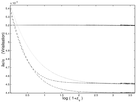
Figure 5: Variation of $\delta\alpha/\alpha$ as a function of $\log(1+z_{v})$. Solid line corresponds to the standard ($\Lambda=0$) $CDM$, dashed line is the $\Lambda CDM$, dashed-dotted line corresponds to a $wCDM$ model with $w_{\phi}=-0.8$, dotted line corresponds to a $wCDM$ model with $w_{\phi}=-0.6$. In all the models, the initial conditions were set in order to have $\alpha_{c}(z=0)=\alpha_{0}$ and to satisfy $\Delta\alpha/\alpha\approx-5.4\times 10^{-6}$ at $3.5\geq|z-z_{v}|\geq 0.5$.

Again, this is because, in a $SCDM$ model, $\Delta_{c}$ is always a constant independent of the redshift at which virialisation occurs. The constancy of $\delta\alpha/\alpha$ is a signature of the $SCDM$ structure-formation model, and it may even provide a means to rule out the $SCDM$ model completely if, when comparing the value of $\delta\alpha/\alpha$ in two different clusters, we do not find the same value, independently of $z_{v}$. A similar result is found for the case of a dark-energy structure formation model at high redshifts where $\delta\alpha/\alpha$ will be constant. This behaviour is expected since at high redshift any $wCDM$ model is asymptotically equivalent to standard $CDM$.

As expected, it is at low redshifts that the difference between $wCDM$ and $SCDM$ emerges. When comparing virialised regions at low redshifts, $\delta\alpha/\alpha$ will increase in a $wCDM$ model as we approach $z=0$. This is due to an increase of the density contrast of the virialised regions, $\Delta_{c}$, and the approach to a constant value of $\alpha_{b}$, see Figure 6.

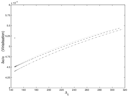
Figure 6: Variation of $\delta\alpha/\alpha$ as a function as a function of $\Delta_{c}$. The single-point corresponds to the standard ($\Lambda=0$) $CDM$, the dashed line is the $\Lambda CDM$, the dash-dot line corresponds to a $wCDM$ model with $w_{\phi}=-0.8$, dotted-line corresponds to a $wCDM$ model with $w_{\phi}=-0.6$. In all the models, the initial conditions were set in order to have $\alpha_{c}(z=0)=\alpha_{0}$ and to satisfy $\Delta\alpha/\alpha\approx-5.4\times 10^{-6}$ at $3.5\geq|z-z_{v}|\geq 0.5$.

In general, the growth will be steeper for smaller values of $w_{\phi}$, although there will be parameter degeneracies between the behaviour of different models, which ensure that there is no simple relation between $\delta\alpha/\alpha$ and the dark-energy equation of state. Note that, independently of the structure formation model we use, $\dot{\alpha}_{c}/\alpha_{c}$ at virialisation is always a decreasing function of time, as shown in Figure 7.

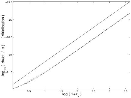
Figure 7: Variation of $log_{10}(\dot{\alpha}/\alpha)$ as a function of $log(1+z_{v})$. Solid line corresponds to the Standard ($\Lambda=0$) $CDM$, dashed-line is the $\Lambda CDM$, dashed-dotted corresponds to a $wCDM$ model with $w_{\phi}=-0.8$, dotted line corresponds to a $wCDM$ model with $w_{\phi}=-0.6$. In all the models, the initial conditions were set in order to have $\alpha_{c}(z=0)=\alpha_{0}$ and to satisfy $\Delta\alpha/\alpha\approx-5.4\times 10^{-6}$ at $3.5\geq|z-z_{v}|\geq 0.5$.

4 The Dependence on the Coupling of $\alpha$-Variation to the Matter Fields

The evolution of $\alpha$ in the background and inside clusters depends mainly on the dominant equation of state of the universe and the sign of the coupling constant $\zeta/\omega,$ which is determined by the theory and the dark matter’s identity. As was shown in (Sandvik, Barrow & Magueijo, 2002; Barrow & Mota, 2002), $\alpha_{b}$ will be nearly constant for an accelerated expansion and also during the radiation era far from the initial singularity (where the kinetic term, $\rho_{\psi}$, can dominate).  Slow evolution of $\alpha$ will occur during the dust-dominated epoch, where $\alpha$ increases logarithmically in time for $\zeta<0$. When $\zeta$ is negative, $\alpha$ will be a slowly growing function of time but $\alpha$ will fall rapidly (even during a curvature-dominated era) for $\zeta$ positive (Sandvik, Barrow & Magueijo, 2002). A similar behaviour is found for the evolution of the fine structure ’constant’ inside overdensities. Thus, we see that a slow change in $\alpha$, cut off by the accelerated expansion at low redshift, that may be required by the data, demands that $\zeta<0$ in the cosmological background.

The sign of $\zeta$ is determined by the physical character of the matter that carries electromagnetic coupling. If it is dominated by magnetic energy then $\zeta<0$, if not then $\zeta>0.$ Baryons will usually have a positive $\zeta$ (although Bekenstein has argued for negative baryonic $\zeta$ in ref. (Bekenstein, 2002), but see (Damour, 2003)), in particular $\zeta\approx 10^{-4}$ for neutrons and protons. Dark matter may have negative values of $\zeta$, for instance superconducting cosmic strings have$\ \zeta\approx-1$.

In the previous section, we have chosen the sign of $\zeta$ to be negative so $\alpha$ is a slowly-growing function in time during the era of dust domination. This was done in order to match the latest observations which suggest that $\alpha$ had a smaller value in the past (Murphy et al., 2001, 2003; Webb et al., 2001, 1999). This is a good approximation, since we have been studying the cosmological evolution of $\alpha$ during large-scale structure formation, when dark matter dominates. However, we know that on sufficiently small scales the dark matter will become dominated by a baryonic contribution for which $\zeta>0.$ The transition in the dominant form of total density, from non-baryonic to baryonic as one goes from large to small scales requires a significant evolution in the magnitude and sign of $\zeta/\omega$. This inhomogeneity will create distinctive behaviours in the evolution of the fine structure ’constant’ and will be studied in more elsewhere. It is clear that a change in the sign of $\zeta/\omega$ will lead to a completely different type of evolution for $\alpha$, although the expected variations in the sign of $\zeta/\omega$ will occur on scales much smaller than those to which we are applying the spherical collapse model here. Hence, we will only investigate the effects of changing the absolute value of the coupling, $|\zeta/\omega|$, for the evolution of the fine structure ’constant’.

From Figure 8 it is clear that the rate of changes in $\alpha_{b}$ and $\alpha_{c}$ will be functions of the absolute value of $\zeta/\omega$. Smaller values of $|\zeta/\omega|$ lead to a slower variation of $\alpha$. A similar behaviour is found for the time variations in $\Delta\alpha/\alpha$, see Figure 9.

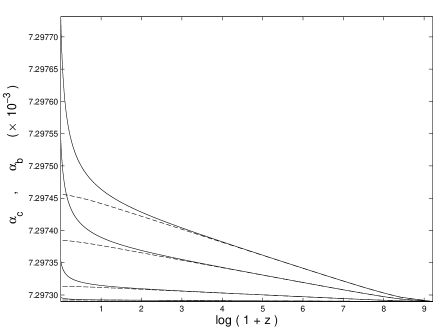
Figure 8: Evolution of $\alpha$ in the background (dashed-line) and inside a cluster (Solid line) as a function of $\log(1+z)$. For $\zeta/\omega=-10^{-8},-4\times 10^{-8},-7\times 10^{-8}$ and $-10^{-9}$. The lower curves correspond to a lower value of $\zeta/\omega$. The initial conditions were set in order to have $\alpha_{c}(z=0)=\alpha_{0}$ and to satisfy $\Delta\alpha/\alpha=-5.4\times 10^{-6}$ at $3\geq|z-z_{v}|\geq 1$, in the case where $\zeta=-7\times 10^{-8}$.

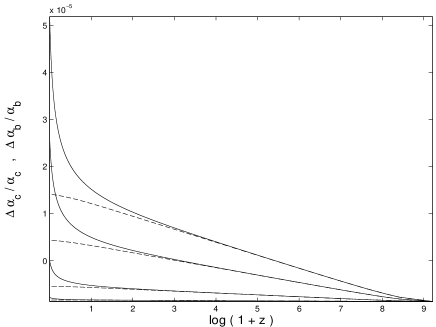
Figure 9: Evolution of $\Delta\alpha/\alpha$ in the background (dashed-line) and inside a cluster (Solid line) as a function of $\log(1+z)$. For $\zeta/\omega=-10^{-8},-4\times 10^{-8},-7\times 10^{-8}$ and $-10^{-9}$. The lower curves correspond to a lower value of $\zeta/\omega$. The initial conditions were set in order to have $\alpha_{c}(z=0)=\alpha_{0}$ and to satisfy $\Delta\alpha/\alpha=-5.4\times 10^{-6}$ at $3\geq|z-z_{v}|\geq 1$, in the case where $\zeta=-7\times 10^{-8}$.

The faster variation in $\alpha$ and $\Delta\alpha/\alpha$ for higher values of $|\zeta/\omega|$ is also a common feature for $\delta\alpha/\alpha$, see Figure 10. This is expected. A stronger coupling to the matter fields would naturally lead to a stronger dependence on the matter inhomogeneities, and in particular on their density contrast, $\Delta_{c}$.

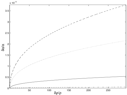
Figure 10: Evolution of $\delta\alpha/\alpha$ as a function $\delta\rho/\rho$. For $\zeta/\omega=-10^{-8},-4\times 10^{-8},-7\times 10^{-8}$ and $-10^{-9}$. The lower curves correspond to a lower value of $\zeta/\omega$. The initial conditions were set in order to have $\alpha_{c}(z=0)=\alpha_{0}$ and to satisfy $\Delta\alpha/\alpha\approx-5.4\times 10^{-6}$ at $3\geq|z-z_{v}|\geq 1$, in the case where $\zeta=-7\times 10^{-8}$.

In reality, the dependence of $\alpha$ on the coupling $\zeta/\omega$ has a degeneracy with respect to the initial condition chosen for $\psi$. This is clear from the scale invariance of equation (3) under linear shifts in the value of $\psi\rightarrow\psi+const$ and rescaling of $\zeta/\omega$ and $t$. It is always possible, to obtain the same evolution (and rate of change) of $\alpha$ and $\Delta\alpha/\alpha$ for any other value of $|\zeta/\omega|$; see for example Tables 1,2,3 and 4, where we have tabulated the shifts $\Delta\alpha/\alpha,\delta\alpha/\alpha,$ and time change, $\dot{\alpha}/\alpha,$ obtained in the clusters and in the background for various numerical choices of $\zeta/\omega$ and virialisation redshift $z_{v}$. The observed Oklo and $\beta$-decay constraints on variations in $\alpha$ are highlighted in italic and boldface, respectively.

$z_{v}$	$\frac{\Delta\alpha}{\alpha}|_{b}\times 10^{-6}$	$\frac{\Delta\alpha}{\alpha}|_{c}\times 10^{-7}$	$\frac{\dot{\alpha}}{\alpha}|_{b}\times 10^{-24}$	$\frac{\dot{\alpha}}{\alpha}|_{c}\times 10^{-22}$	$\frac{\delta\alpha}{\alpha}\times 10^{-6}$
$0.00$	$-5.381$	$0.000$	$0.361$	$1.068$	$5.38$
$\mathit{0.09}$	$\mathit{-5.397}$	$\mathit{\ -1.618}$	$\mathit{\ 0.427}$	$\mathit{\ 1.128}$	$\mathit{\ 5.24}$
$0.18$	$-5.412$	$-2.889$	$0.493$	$1.192$	$5.12$
$0.34$	$-5.442$	$-4.769$	$0.623$	$1.329$	$4.97$
$\mathbf{0.41}$	$\mathbf{-5.456}$	$\mathbf{-5.485}$	$\mathbf{\ 0.688}$	$\mathbf{\ 1.401}$	$\mathbf{\ 4.91}$
$0.51$	$-5.474$	$-6.271$	$0.773$	$1.498$	$4.85$
$1.07$	$-5.572$	$-9.139$	$1.303$	$2.161$	$4.66$
$2.14$	$-5.722$	$-11.658$	$2.508$	$3.821$	$4.56$
$3.31$	$-5.843$	$-13.129$	$4.055$	$6.043$	$4.53$
$4.83$	$-5.961$	$-14.415$	$6.407$	$9.466$	$4.52$

Table 1: Time and space variations in $\alpha$ obtained for the corresponding redshifts of virialisation, $z_{v}$, for $\zeta/\omega=-10^{-1}$. We have assumed a $\Lambda CDM$ model. The indexes ${}^{\prime}b^{\prime}$ and ${}^{\prime}c^{\prime}$, stand for background and cluster respectively. The italic and bold entries correspond approximately to the level of the Oklo and $\beta$-decay rate constraints, respectively. The quasar absorption spectra observations correspond to the values of $\Delta\alpha/\alpha|_{b}$. The initial conditions were set in order to have $\alpha_{c}(z=0)=\alpha_{0}$.

$z_{v}$	$\frac{\Delta\alpha}{\alpha}|_{b}\times 10^{-6}$	$\frac{\Delta\alpha}{\alpha}|_{c}\times 10^{-7}$	$\frac{\dot{\alpha}}{\alpha}|_{b}\times 10^{-24}$	$\frac{\dot{\alpha}}{\alpha}|_{c}\times 10^{-22}$	$\frac{\delta\alpha}{\alpha}\times 10^{-6}$
$0.00$	$-5.382$	$0.000$	$0.361$	$1.068$	$5.38$
$\mathit{0.09}$	$\mathit{-5.398}$	$\mathit{\ -1.618}$	$\mathit{\ 0.427}$	$\mathit{\ 1.128}$	$\mathit{\ 5.24}$
$0.18$	$-5.414$	$-2.889$	$0.493$	$1.193$	$5.12$
$0.34$	$-5.443$	$-4.769$	$0.623$	$1.329$	$4.97$
$\mathbf{0.41}$	$\mathbf{-5.458}$	$\mathbf{\ -5.486}$	$\mathbf{\ 0.688}$	$\mathbf{\ 1.401}$	$\mathbf{\ 4.91}$
$0.51$	$-5.476$	$-6.272$	$0.773$	$1.498$	$4.85$
$1.07$	$-5.573$	$-9.141$	$1.303$	$2.161$	$4.66$
$2.14$	$-5.723$	$-11.660$	$2.508$	$3.822$	$4.56$
$3.31$	$-5.844$	$-13.132$	$4.056$	$6.045$	$4.53$
$4.83$	$-5.962$	$-14.418$	$6.408$	$9.469$	$4.52$

Table 2: Time and space variations in $\alpha$ for the corresponding redshifts of virialisation, $z_{v},$ with $\zeta/\omega=-10^{-5}$ .We assumed a $\Lambda CDM$ model. The indices ${}^{\prime}b^{\prime}$ and ${}^{\prime}c^{\prime}$, stand for background and cluster respectively. The italic and bold entries correspond approximately to the Oklo and $\beta$-decay rate constraints, respectively. The initial conditions were set in order to have $\alpha_{c}(z=0)=\alpha_{0}$.

$z_{v}$	$\frac{\Delta\alpha}{\alpha}|_{b}\times 10^{-6}$	$\frac{\Delta\alpha}{\alpha}|_{c}\times 10^{-7}$	$\frac{\dot{\alpha}}{\alpha}|_{b}\times 10^{-24}$	$\frac{\dot{\alpha}}{\alpha}|_{c}\times 10^{-22}$	$\frac{\delta\alpha}{\alpha}\times 10^{-6}$
$0.00$	$-5.381$	$0.000$	$0.361$	$1.068$	$5.38$
$\mathit{0.09}$	$\mathit{-5.397}$	$\mathit{\ -1.617}$	$\mathit{\ 0.427}$	$\mathit{\ 1.128}$	$\mathit{\ 5.24}$
$0.18$	$-5.413$	$-2.889$	$0.493$	$1.192$	$5.12$
$0.34$	$-5.442$	$-4.768$	$0.623$	$1.329$	$4.97$
$\mathbf{0.41}$	$\mathbf{-5.457}$	$\mathbf{\ -5.485}$	$\mathbf{\ 0.688}$	$\mathbf{\ 1.401}$	$\mathbf{\ 4.91}$
$0.51$	$-5.475$	$-6.271$	$0.773$	$1.498$	$4.85$
$1.07$	$-5.572$	$-9.139$	$1.303$	$2.161$	$4.66$
$2.14$	$-5.722$	$-11.658$	$2.508$	$3.822$	$4.56$
$3.31$	$-5.843$	$-13.129$	$4.056$	$6.044$	$4.53$
$4.83$	$-5.961$	$-14.415$	$6.407$	$9.467$	$4.52$

Table 3: Time and space variations in $\alpha$ for the corresponding redshifts of virialisation, $z_{v},$ for $\zeta/\omega=-10^{-9}$ .We have assumed a $\Lambda CDM$ model. The indices ${}^{\prime}b^{\prime}$ and ${}^{\prime}c^{\prime}$, stand for background and cluster respectively. The italic and bold entries correspond approximately to the Oklo and to the $\beta$-decay rate constraints, respectively. The initial conditions were set in order to have $\alpha_{c}(z=0)=\alpha_{0}$.

$z_{v}$	$\frac{\Delta\alpha}{\alpha}|_{b}\times 10^{-6}$	$\frac{\Delta\alpha}{\alpha}|_{c}\times 10^{-7}$	$\frac{\dot{\alpha}}{\alpha}|_{b}\times 10^{-24}$	$\frac{\dot{\alpha}}{\alpha}|_{c}\times 10^{-22}$	$\frac{\delta\alpha}{\alpha}\times 10^{-6}$
$0.00$	$-5.385$	$0.000$	$0.361$	$1.068$	$5.38$
$\mathit{0.09}$	$\mathit{-5.401}$	$\mathit{\ -1.619}$	$\mathit{\ 0.428}$	$\mathit{\ 1.129}$	$\mathit{\ 5.24}$
$0.18$	$-5.416$	$-2.891$	$0.493$	$1.193$	$5.13$
$0.34$	$-5.446$	$-4.772$	$0.624$	$1.330$	$4.97$
$\mathbf{0.41}$	$\mathbf{-5.460}$	$\mathbf{\ -5.489}$	$\mathbf{\ 0.689}$	$\mathbf{\ 1.402}$	$\mathbf{\ 4.91}$
$0.51$	$-5.478$	$-6.275$	$0.773$	$1.499$	$4.85$
$1.07$	$-5.576$	$-9.145$	$1.304$	$2.162$	$4.66$
$2.14$	$-5.726$	$-11.666$	$2.510$	$3.824$	$4.56$
$3.31$	$-5.847$	$-13.138$	$4.058$	$6.048$	$4.53$
$4.83$	$-5.965$	$-14.425$	$6.412$	$9.473$	$4.52$

Table 4: Time and space variations in $\alpha$ for the redshifts of virialisation, $z_{v}$, for $\zeta/\omega=-10^{-13}$. We have assumed a $\Lambda CDM$ model. The indices ${}^{\prime}b^{\prime}$ and ${}^{\prime}c^{\prime}$, stand for background and cluster respectively. The italic and bold entries correspond approximately to the Oklo and $\beta$-decay rate constraints, respectively. The initial conditions were set in order to have $\alpha_{c}(z=0)=\alpha_{0}$.

In the plots of this section, we have chosen the value $\zeta/\omega=-7\times 10^{-8}$ to be the one which satisfies the current observations, but we could have used any value of $|\zeta/\omega|$ because of the invariance under rescalings. However, once we set the initial condition for a given value of $\zeta/\omega$, any deviation from that value leads to quite different future variations in $\alpha$. This can occur if there are regions of the universe where the dominant matter has a different nature, and and do possesses a different value (and even sign) of $\zeta/\omega$ to that in our solar system. The evolution of $\alpha$ in those regions may then be different from the one that led to the value of $\alpha_{c}(z=z_{v})=\alpha_{0}$ on Earth.

It is important to note that, due to the degeneracy between the initial condition and the coupling to the matter fields, there is no way to avoid evolving differences in $\alpha$ variations between the overdensities and the background. The difference will be of the same order of magnitude as the effects indicated by the recent quasar absorption-line data. This is not a coincidence and it is related to the fact that we have normalised $\alpha(z=z_{v})=\alpha_{0}$ on Earth and $\Delta\alpha/\alpha=5.4\times 10^{-6}$ at $3.5\geq|z-z_{v}|\geq 0.5$. So, any varying-$\alpha$ model that uses these normalisations will create a similar difference in $\alpha$ evolution between the overdensities and the background, independently of the coupling $\zeta/\omega$.

We might ask: how model-independent are these results? In this connection it is interesting to note that even with a zero coupling to the matter fields (which is unrealistic), $\zeta=0$, there is no way to avoid difference arising between the evolution of $\alpha$ in the background and in the cluster overdensities. While the background expansion has a monotonically-increasing scale factor, $a(t)$, the overdensities will have a scale radius, $R(t)$, which will eventually collapse at a finite time. For instance, in the case where $\zeta=0$, equations (3) and (5) can be automatically integrated to give:

$$\dot{\psi}\propto a^{-3}\qquad,\qquad\dot{\psi}_{c}\propto R^{-3}$$ (18)

The difference between those two solutions clearly increases, especially after the turnaround of the overdensity, when that region starts to collapse. As the collapse proceeds, the bigger will be the difference between the background and the overdensity. Variations in $\alpha$ between the background and the overdensities are therefore quite natural although they have always been ignored in studies of varying constants in cosmology.

5 Discussion of the Results and Observational Constraints

The development of matter inhomogeneities in our universe affects the cosmological evolution of the fine structure ’constant’ (Barrow & Mota, 2003; Mota & Barrow, 2003). Therefore, variations in $\alpha$ depend on nature of its coupling to the matter fields and the detailed large-scale structure formation model. Large-scale structure formation models depend in turn on the dark-energy equation of state. This dependence is particularly strong at low redshifts, when dark energy dominates the density of the universe (Lahav et al., 1991; Wang & Steinhardt, 1998). Using the BSBM varying-$\alpha$ theory, and the simplest spherical collapse model, we have studied the effects of the dark-energy equation of state and the coupling to the matter fields on the evolution of the fine structure ’constant’. We have compared the evolution of $\alpha$ inside virialised overdensities, using the standard ($\Lambda=0$) $CDM$ model of structure formation and dark-energy modification ($wCDM$). It was shown that, independently of the model of structure formation one considers, there is always a spatial contrast, $\delta\alpha/\alpha$, between $\alpha$ in an overdensity and in the background. In a $SCDM$ model, $\delta\alpha/\alpha$ is always a constant, independent of the virialisation redshift, see Table 5. In the case of a $wCDM$ model, especially at low redshifts, the spatial contrast depends on the time when virialisation occurs and the equation of state of the dark energy. At high redshifts, when the $wCDM$ model becomes asymptotically equivalent to the $SCDM$ one, $\delta\alpha/\alpha$ is a constant. At low redshifts, when dark energy starts to dominate, the difference between $\alpha$ in a cluster and in the background grows. The growth rate is proportional to $|w_{\phi}|$, see Tables 6, 7 and 8. These differences in the behaviour of the fine structure ’constant’, its ’time shift density contrast’ ($\Delta\alpha/\alpha$) and its ’spatial density contrast’ ($\delta\alpha/\alpha$) could help us to distinguish among different dark-energy models of structure formation at low redshifts.

$z_{v}$	$\frac{\Delta\alpha}{\alpha}|_{b}\times 10^{-6}$	$\frac{\Delta\alpha}{\alpha}|_{c}\times 10^{-7}$	$\frac{\dot{\alpha}}{\alpha}|_{b}\times 10^{-24}$	$\frac{\dot{\alpha}}{\alpha}|_{c}\times 10^{-22}$	$\frac{\delta\alpha}{\alpha}\times 10^{-6}$
$0.00$	$-5.203$	$0.000$	$0.959$	$1.409$	$5.20$
$0.06$	$-5.229$	$-0.266$	$1.047$	$1.537$	$5.20$
$\mathit{0.12}$	$\mathit{-5.254}$	$\mathit{-0.517}$	$\mathit{\ 1.137}$	$\mathit{\ 1.670}$	$\mathit{\ 5.20}$
$0.38$	$-5.349$	$-1.463$	$1.553$	$2.281$	$5.20$
$\mathbf{0.46}$	$\mathbf{-5.374}$	$\mathbf{-1.717}$	$\mathbf{\ 1.690}$	$\mathbf{\ 2.481}$	$\mathbf{\ 5.20}$
$0.54$	$-5.399$	$-1.962$	$1.830$	$2.687$	$5.20$
$1.07$	$-5.534$	$-3.313$	$2.859$	$4.198$	$5.20$
$2.12$	$-5.720$	$-5.175$	$5.273$	$7.744$	$5.20$
$3.00$	$-5.834$	$-6.315$	$7.668$	$11.261$	$5.20$
$4.92$	$-6.012$	$-8.102$	$13.824$	$20.305$	$5.20$

Table 5: $(\Lambda=0)$ CDM: Time and space variations in $\alpha$ for the corresponding redshifts of virialisation, $z_{v}$, in the $(\Lambda=0)$ standard Cold Dark Matter model. The indexes ${}^{\prime}b^{\prime}$ and ${}^{\prime}c^{\prime}$, stand for background and cluster respectively. The italic and bold entries correspond approximately to the Oklo and to the $\beta$-decay rate constraint, respectively. The quasar absorption spectra observations correspond to the values of $\Delta\alpha/\alpha|_{b}$. The initial conditions were set for $\zeta/\omega=-2\times 10^{-8}$, in order to have $\alpha_{c}(z=0)=\alpha_{0}$.

$z_{v}$	$\frac{\Delta\alpha}{\alpha}|_{b}\times 10^{-6}$	$\frac{\Delta\alpha}{\alpha}|_{c}\times 10^{-7}$	$\frac{\dot{\alpha}}{\alpha}|_{b}\times 10^{-24}$	$\frac{\dot{\alpha}}{\alpha}|_{c}\times 10^{-22}$	$\frac{\delta\alpha}{\alpha}\times 10^{-6}$
$0.00$	$-5.440$	$0.000$	$0.332$	$1.036$	$5.44$
$0.08$	$-5.453$	$-1.130$	$0.385$	$1.121$	$5.34$
$\mathit{0.17}$	$\mathit{-5.466}$	$\mathit{\ -2.077}$	$\mathit{\ 0.440}$	$\mathit{\ 1.207}$	$\mathit{\ 5.26}$
$0.25$	$-5.478$	$-2.886$	$0.497$	$1.293$	$5.19$
$\mathbf{0.40}$	$\mathbf{-5.502}$	$\mathbf{\ -4.208}$	$\mathbf{\ 0.613}$	$\mathbf{\ 1.469}$	$\mathbf{\ 5.08}$
$0.50$	$-5.517$	$-4.914$	$0.691$	$1.586$	$5.03$
$1.08$	$-5.599$	$-7.828$	$1.217$	$2.354$	$4.82$
$2.02$	$-5.710$	$-10.372$	$2.238$	$3.831$	$4.67$
$3.02$	$-5.806$	$-11.980$	$3.518$	$5.684$	$4.61$
$4.59$	$-5.924$	$-13.626$	$5.876$	$9.107$	$4.56$

Table 6: $w=-0.6$ CDM: Time and space variations in $\alpha$ for the corresponding redshifts of virialisation, $z_{v}$, in the $w=-0.6$ CDM model . The indices ${}^{\prime}b^{\prime}$ and ${}^{\prime}c^{\prime}$, stand for background and cluster respectively. The italic and bold entries correspond approximately to the Oklo and $\beta$-decay rate constraints, respectively. The quasar absorption spectra observations correspond to the values of $\Delta\alpha/\alpha|_{b}$. The initial conditions were set for $\zeta/\omega=-2\times 10^{-8}$, in order to have $\alpha_{c}(z=0)=\alpha_{0}$.

$z_{v}$	$\frac{\Delta\alpha}{\alpha}|_{b}\times 10^{-6}$	$\frac{\Delta\alpha}{\alpha}|_{c}\times 10^{-7}$	$\frac{\dot{\alpha}}{\alpha}|_{b}\times 10^{-24}$	$\frac{\dot{\alpha}}{\alpha}|_{c}\times 10^{-22}$	$\frac{\delta\alpha}{\alpha}\times 10^{-6}$
$0.00$	$-5.412$	$0.000$	$0.340$	$1.078$	$5.41$
$\mathit{0.09}$	$\mathit{-5.427}$	$\mathit{\ -1.587}$	$\mathit{\ 0.401}$	$\mathit{\ 1.148}$	$\mathit{\ 5.27}$
$0.18$	$-5.441$	$-2.857$	$0.462$	$1.220$	$5.16$
$0.34$	$-5.468$	$-4.777$	$0.586$	$1.370$	$4.99$
$\mathbf{0.42}$	$\mathbf{-5.481}$	$\mathbf{\ -5.527}$	$\mathbf{\ 0.649}$	$\mathbf{\ 1.447}$	$\mathbf{\ 4.93}$
$0.52$	$-5.498$	$-6.362$	$0.731$	$1.549$	$4.86$
$1.09$	$-5.587$	$-9.516$	$1.260$	$2.239$	$4.64$
$2.01$	$-5.706$	$-11.997$	$2.247$	$3.595$	$4.51$
$3.38$	$-5.841$	$-13.948$	$4.023$	$6.125$	$4.45$
$4.92$	$-5.953$	$-15.297$	$6.362$	$9.510$	$4.42$

Table 7: $w=-0.8$ CDM: Time and space variations in $\alpha$ for the corresponding redshifts of virialisation, $z_{v},$ for the $w=-0.8$ CDM model. The indices ${}^{\prime}b^{\prime}$ and ${}^{\prime}c^{\prime}$, stand for background and cluster respectively. The italic and bold entries correspond approximately to the Oklo and $\beta$-decay rate constraints, respectively. The quasar absorption spectra observations correspond to the values of $\Delta\alpha/\alpha|_{b}$. The initial conditions were set for $\zeta/\omega=-2\times 10^{-8}$, in order to have $\alpha_{c}(z=0)=\alpha_{0}$.

$z_{v}$	$\frac{\Delta\alpha}{\alpha}|_{b}\times 10^{-6}$	$\frac{\Delta\alpha}{\alpha}|_{c}\times 10^{-7}$	$\frac{\dot{\alpha}}{\alpha}|_{b}\times 10^{-24}$	$\frac{\dot{\alpha}}{\alpha}|_{c}\times 10^{-22}$	$\frac{\delta\alpha}{\alpha}\times 10^{-6}$
$0.00$	$-5.382$	$0.000$	$0.361$	$1.068$	$5.38$
$\mathit{0.09}$	$\mathit{-5.398}$	$\mathit{\ -1.618}$	$\mathit{\ 0.427}$	$\mathit{\ 1.128}$	$\mathit{\ 5.24}$
$0.18$	$-5.414$	$-2.889$	$0.493$	$1.193$	$5.12$
$0.34$	$-5.443$	$-4.769$	$0.623$	$1.329$	$4.97$
$\mathbf{0.41}$	$\mathbf{-5.458}$	$\mathbf{-5.486}$	$\mathbf{0.688}$	$\mathbf{1.401}$	$\mathbf{4.91}$
$0.51$	$-5.476$	$-6.272$	$0.773$	$1.498$	$4.85$
$1.07$	$-5.573$	$-9.141$	$1.303$	$2.161$	$4.66$
$2.14$	$-5.723$	$-11.660$	$2.508$	$3.822$	$4.56$
$3.31$	$-5.844$	$-13.132$	$4.056$	$6.045$	$4.53$
$4.83$	$-5.962$	$-14.418$	$6.408$	$9.469$	$4.52$

Table 8: $\Lambda$ CDM: Time and space variations in $\alpha$ for the corresponding redshifts of virialisation, $z_{v}$, in the $\Lambda CDM$ model. The indices ${}^{\prime}b^{\prime}$ and ${}^{\prime}c^{\prime}$, stand for background and cluster respectively. The italic and bold entries correspond approximately to the Oklo and $\beta$-decay rate constraints, respectively. The quasar absorption spectra observations correspond to the values of $\Delta\alpha/\alpha|_{b}$. The initial conditions were set for $\zeta/\omega=-2\times 10^{-8}$, in order to have $\alpha_{c}(z=0)=\alpha_{0}$.

Variations in $\alpha$ also depend on the value and sign of the coupling, $\zeta/\omega$, of the scalar field responsible for variations in $\alpha$, to the matter fields. A higher value of $|\zeta/\omega|$, leads to a stronger dependence on the density contrast of the matter inhomogeneities. If the value or sign of $\zeta/\omega$ changes in space, then spatial inhomogeneities in $\alpha$ occur. This could happen if we take into account that on small enough scales, baryons will dominate the dark matter density. The sign and value of $\zeta/\omega$ will change, and variations in $\alpha$ will evolve differently on different scales. If there are no variations in the sign and value of $\zeta/\omega$, then the only spatial variations in $\alpha$ are the ones resulting from the dependence of the fine structure ’constant’ on the density contrast of the region in which one is measuring $\alpha$. At first sight, one might conclude that the difference between $\alpha_{c}$ and $\alpha_{b}$, is only a consequence of the coupling of $\alpha$ to matter. In reality this is not so. It is always possible to obtain the same results for any value $|\zeta/\omega|$ with a suitable choice of initial conditions, as can be seen from the results in Tables 1, 2, 3 and 4.

The results of this paper offer a natural explanation for why any experiment carried out on Earth (Fujii et al, 2000; Prestage, Tjoelker & Maleki, 1995; Sortais et al., 2001), or in our local solar system (Olive et al., 2002), gives constraints on possible time-variation in $\alpha$ that are much stronger than the magnitude of variation that is consistent with the quasar observations (Murphy, Webb & Flambaum, 2003) on extragalactic scales. The value of the fine structure ’constant’ on Earth, and most probably in our local cluster, differs from that in the background universe because of the different histories of these regions. It can be seen from the Tables 5, 6, 7 and 8 that inside a virialised overdensity we expect $\Delta\alpha/\alpha\approx-10^{-7}$ for $z_{v}\leq 1,$ while in the background we have $\Delta\alpha/\alpha\approx-10^{-6}$, independently of the structure formation model used. The same conclusions arise independently of the absolute value of the coupling $\zeta/\omega$, see Tables 1, 2, 3 and 4.

The dependence of $\alpha$ on the matter-field perturbations is much less important when one is studying effects of varying $\alpha$ on the early universe, for example on the last scattering of the CMB or the course of primordial nucleosynthesis (Martins et al., 2003; Avelino et al., 2000; Battye, Crittenden & Weller, 2001). In the linear regime of the cosmological perturbations, small perturbations in $\alpha$ will decay or become constant in the radiation era (Barrow & Mota, 2003). At the redshift of last scattering, $z=1100$, it was found in (Mota & Barrow, 2003) that $\Delta\alpha/\alpha\leq 10^{-5}$. In the background, the fine structure ’constant’, will be a constant during the radiation era (Sandvik, Barrow & Magueijo, 2002) so long as the kinetic term is negligible. A growth in value of $\alpha$ will occur only in the matter-dominated era (Barrow & Mota, 2002). Hence, the early-universe constraints, coming from the CMB and primordial nucleosynthesis, are comparatively weak, $\Delta\alpha/\alpha\leq 10^{-2}$, and are easily satisfied.

Appendix A BSBM Equations

From the BSBM action (1) the equation of motion for $\psi$ comes

$$\Box\psi=\frac{2}{\omega}e^{-2\psi}{\mathcal{L}}_{em}$$ (19)

The right-hand-side (RHS) of equation (19) represents a source term for $\psi$, which includes all the matter fields which are coupled to it. These include not only relativistic matter (like photons), but as well as non-relativistic one that interact electromagnetically. It is clear that ${\cal{L}}_{em}$, vanishes for a sea of pure radiation since ${\cal{L}}_{em}=\left(E^{2}-B^{2}\right)/2=0$. The only significant contribution to a variation in $\psi$ comes from nearly pure electrostatic or magnetostatic energy associated to non-relativistic particles. In order to make quantitative predictions we then need to know how much of the non-relativistic matter contributes to the right-hand-side (RHS) of equation (19). This can be parametrised by the ratio $\zeta={\cal{L}}_{em}/\rho_{m}$, where $\rho_{m}$ is the energy density of the non-relativistic matter. This non-relativistic matter, which interact electromagnetically, contributes to the Friedman equation (2) as $\rho_{m}|\zeta|e^{-2\psi}$.

For protons and neutrons, $\zeta$ can be estimated from the electromagnetic corrections to the nucleon mass, $0.63MeV$ and $-0.13Mev$, respectively (Dvali & Zaldarriaga, 2002). This correction contains the $E^{2}/2$ contribution, which is always positive, and also term of the form $j_{\mu}a^{\mu}$, where $j_{\mu}$ is the quarks’ current (Sandvik, Barrow & Magueijo, 2002). Hence we take a guidance value of $\zeta\approx 10^{-4}$ for protons and neutrons.

Using the parameter $\zeta$, the fraction of electric and magnetic energies may then be written as (Sandvik, 2002):

$$\zeta^{E}=\frac{E^{2}}{\rho_{m}}\qquad,\qquad\zeta^{B}=\frac{B^{2}}{\rho_{m}}$$ (20)

where $E^{2}$ and $B^{2}$ are the electric and magnetic energies respectively. Using (20) in equation (19) we have (Sandvik, 2002)

$$\Box\psi=\frac{2}{\omega}e^{-2\psi}\rho_{m}\left(\zeta^{E}-\zeta^{B}\right)$$ (21)

Since we are interested in the cosmological evolution of $\alpha$, instead of using both parameters $\zeta^{E}$ and $\zeta^{B}$, we will use throughout this articles, the cosmological parameter, $\zeta$, defined as $\zeta\equiv\zeta^{E}-\zeta^{B}$, which in the limit where $\zeta^{E}\gg\zeta^{B}$ is positive, and when $\zeta^{E}\ll\zeta^{B}$ is negative. Note that, the cosmological value of $\zeta$ has to be weighted, not only by the electromagnetic-interacting baryon fraction, but also by the fraction of matter that is non-baryonic. Hence the value and sign of $\zeta$ depends strongly on the nature of dark matter to which the field $\psi$ might be coupled.

Appendix B The BSBM model and WEP violations

In BSBM the test-particle Lagrangian may be split as $\mathcal{L}_{t}=\mathcal{L}_{m}+e^{-2\psi}\mathcal{L}_{em}$. Variation with respect to the metric leads to a similar split of the stress-energy tensor, producing an energy density of the form $\rho((1-\zeta_{t})+\zeta_{t}e^{-2\psi}),$ and so a mass of $m((1-\zeta_{t})+\zeta_{t}e^{-2\psi}),$ (assuming electric fields dominate). In order to preserve their ratios of $\zeta_{t}=\mathcal{L}_{em}/\rho$ test particles may thus be represented by (Magueijo, Barrow & Sandvik, 2002)

$$\mathcal{L}(y)=-\int d\tau\;m((1-\zeta_{t})-\zeta_{t}e^{-2\psi})[-g_{\mu\nu}\dot{x}^{\mu}\dot{x}^{\nu}]^{\frac{1}{2}}{\frac{\delta(x-y)}{\sqrt{-g}}}$$ (22)

where over-dots are derivatives with respect to the proper time $\tau$. This leads to equations of motion:

$$\ddot{x}^{\mu}+\Gamma_{\alpha\beta}^{\mu}\dot{x}^{\alpha}\dot{x}^{\beta}+{\frac{2\zeta_{t}e^{-2\psi}}{(1-\zeta_{t})-\zeta_{t}e^{-2\psi}}}\partial^{\mu}\psi=0$$ (23)

which in the non-relativistic limit (with $\zeta_{t}\ll 1$) reduce to

$${\frac{d^{2}x^{i}}{dt^{2}}}=-\nabla_{i}\phi-2\zeta_{t}\nabla_{i}\psi\;,$$ (24)

where $\phi$ is the gravitational potential. Thus we predict an anomalous acceleration:

$$a={\frac{M_{s}}{r^{2}}}{\left(1+{\frac{\zeta_{s}\zeta_{t}}{\omega\pi}}\right)}$$ (25)

Violations of the WEP occur because $\zeta_{t}$ is substance dependent. For two test bodies with $\zeta_{1}$ and $\zeta_{2}$ the Eötvös parameter is:

$$\eta\equiv{\frac{2|a_{1}-a_{2}|}{a_{1}+a_{2}}}={\frac{\zeta_{s}|\zeta_{1}-\zeta_{2}|}{\omega\pi}.}$$ (26)

This can be written more conveniently as the product of the following 3 factors (Sandvik, Barrow & Magueijo, 2002):

$$\eta=\left({\frac{\zeta_{E}|\zeta_{1}-\zeta_{2}|}{\pi\zeta_{p}}}\ \right)\left({\frac{\zeta_{p}}{\zeta}}\right)\left({\frac{\zeta}{\omega}}\right).$$ (27)

where $E$ denotes Earth. If we take $\zeta_{n}\approx\zeta_{p}\approx|\zeta_{p}-\zeta_{n}|=\mathcal{O}(10^{-4})$ then for typical substances the first factor is $\approx 10^{-5}$. In order to satisfy the existing WEP violations experimental bounds (Will, 2001; Nordtvedt, 2002), we need to “play around” with the two last terms of equation (27). If we use the value assumed in (Sandvik, Barrow & Magueijo, 2002) $\zeta/\omega\approx-10^{-4}$. Hence, we need $\zeta=\mathcal{O}(1)$ to produce $\eta=\mathcal{O}(10^{-13}),$ just an order of magnitude below existing experimental bounds. If we instead use $\zeta/\omega\approx-10^{-8}$ we would need $\zeta=\mathcal{O}(10^{-4})$ to satisfy the same experimental bounds. The choice in the value of $\zeta/\omega$ just depends on the nature of dark-matter, but this is beyond the scope of this paper. Nevertheless, as shown in this paper, any choice of $\zeta_{/}\omega$ will give us the same cosmological behaviour for $\Delta\alpha/\alpha$ due to a degeneracy with the initial conditions for $\psi$. Hence, the results presented in this paper are not affected at all by any experimental constraint imposed by WEP violations.

References

- Anchordoqui & Goldberg (2003) Anchordoqui L., Goldberg H., 2003, arXiv:hep-ph/0306084
- Armendariz-Picon (2002) Armendariz-Picon C., 2002, Phys. Rev. D 66, 064008
- Avelino et al. (2000) Avelino et al., 2000, Phys. Rev. D 62 123508;
- Bahcall, Steinhardt, & D.Schlegel (2003) Bahcall J.N., Steinhardt C.L., Schlegel D.,2003 arXiv:astro-ph/0301507
- Banks, Dine & Douglas (2002) Banks T., Dine M., Douglas M.R., 2002, Phys. Rev. Lett. 88, 131301
- Barrow (2002) Barrow J.D., 2002,The Constants of Nature: From Alpha to Omega, London: J. Cape
- Barrow & O’Toole (1999) Barrow J.D. , O’Toole C., 1999, arXiv:astro-ph/9904116;
- Barrow, Magueijo & Sandvik (2002a) Barrow J.D., Magueijo J. , Sandvik H.B., 2002a, Int. J. Mod. Phys. D 11 1615;
- Barrow, Magueijo & Sandvik (2002b) Barrow J.D., Magueijo J. , Sandvik H.B., 2002b, Phys. Rev. D 66, 043515
- Barrow, Sandvik & Magueijo (2002a) Barrow J.D., Sandvik H.B. , Magueijo J., 2002a, Phys. Rev. D 65, 063504
- Barrow, Sandvik & Magueijo (2002b) Barrow J.D., Sandvik H.B. , Magueijo J., 2002b, Phys. Rev. D 65, 123501
- Barrow & Mota (2002) Barrow J.D. , Mota D.F., 2002, Class. Quant. Grav. 19, 6197
- Barrow & Mota (2003) Barrow J.D. , Mota D.F., 2003, Class. Quant. Grav. 20, 2045
- Battye, Crittenden & Weller (2001) Battye R., Crittenden R., Weller J., 2001, Phys. Rev. D 63 043505
- Bekenstein (1982) Bekenstein J.D., 1982, Phys. Rev. D 25, 1527
- Bekenstein (2002) Bekenstein J.D., 2002, Phys. Rev. D 66, 123514
- Bekenstein (2003) Bekenstein J.D., 2003, astro-ph/0301566
- Boehm et al. (2002) Boehm C. et al., 2002, Phys. Rev. D66 083505
- Brax et al. (2003) Brax P., et al., 2003, Astrophys. Space Sci. 283, 627
- Calmet & Fritzsch (2002a) Calmet X., Fritzsch H., 2002a, Phys. Lett. B 540, 173
- Calmet & Fritzsch (2002b) Calmet X., Fritzsch F., 2002b, Eur. Phys. J. C 24, 639
- (22) Copeland E.J., Nunes N.J., Pospelov M., 2003, arXiv:hep-ph/0307299.
- Cowie & Songaila (1995) L. L. Cowie , A. Songaila, Ap. J. 453, 596 (1995)
- Damour & Polyakov (1994) Damour T., Polyakov A.M., 1994, Nucl. Phys. B 423, 532
- Damour (2003) Damour T., 2003, arXiv:gr-qc/0306023.
- Damour & Dyson (1996) Damour T., Dyson F., 1996, Nucl. Phys. B 480, 37
- Darling (2003) Darling, J.,2003, Phys. Rev. Lett. 91, 011301
- Dent (2003) Dent T., 2003 , arXiv:hep-ph/0305026
- Dent & Fairbairn (2003) Dent T. , Fairbairn M., 2003, Nucl. Phys. B 653, 256
- Dvali & Zaldarriaga (2002) Dvali G.R., Zaldarriaga M., 2002, Phys. Rev. Lett. 88 , 091303
- Fujii et al (2000) Fujii Y. et al., 2000, Nucl. Phys. B 573, 377
- Fujii (2003) Fujii Y., 2003, arXiv:astro-ph/0307263;
- Fujii & Iwanoto (2003) Fujii Y. and Iwanoto A., 2003, hep-ph0309087
- Fritzsch (2002) Fritzsch H., 2002 hep-ph/0212186;
- Hannestad (1999) Hannestad S., 1999, Phys.Rev.D60:023515
- Huang & Li (2002) Huang Q.G., Li M., 2003, JHEP 0305 026
- Ivanchik, Potekhin & Varshalovich (1999) Ivanchik I.V., Potekhin A.Y., Varshalovich D.A., 1999, A & A 343, 439
- Kaplinghat, Scherrer & Turner (1999) Kaplinghat M., Scherrer R.J. & Turner M. S., 1999, Phys.Rev.D60:023516
- Kostelecky, Lehnert & Perry (2002) Kostelecky A., Lehnert R. & Perry M., 2002, ”Spacetime-varying couplings and Lorentz violation”, astro-ph/0212003
- Lahav et al. (1991) Lahav O. et al., 1991, Mon. Not. Roy. Astron. Soc. 251 128;
- Lamoreaux (2003) Lamoreaux S., 2003, nucl-th/0309048.
- Landau & Lifshitz (1975) Landau L., Lifshitz E., 1975, The Classical Theory of Fields, 4th. ed. Pergamon, Oxford
- Langacker, Segre & Strassler (2002) Langacker P., Segre G., Strassler M.J., 2002, Phys. Lett. B528, 121
- Levshakov (1994) Levshakov S.A., 1994, Mon. Not. R.astron. Soc. 269, 339
- Magueijo, Barrow & Sandvik (2002) Magueijo J., Barrow J.D. , Sandvik H., 2002, Phys. Lett. B 549, 284
- Marciano (1984) Marciano W.J., 1984, Phys. Rev. Lett. 52, 489
- Marion et al. (2002) Marion et al., 2003, Phys. Rev. Lett. 90, 150801
- Martins et al. (2003) Martins et al., 2003, arXiv:astro-ph/0302295;
- Mota & Barrow (2003) Mota D.F., Barrow J.D., 2003, arXiv:astro-ph/0306047.
- Murphy et al. (2001) Murphy M.T. et al.,2001, MNRAS, 327, 1208
- Murphy et al. (2003) Murphy M.T. et al., 2003, Astrophys. Space Sci. 283, 577
- Murphy, Flambaum & Webb (2003) Murphy M.T., Flambaum V.V., Webb J.K., 2003, Lecture Notes in Physics, Proc. 302 WE Heraeus Seminar: Astrophysics, Clocks and Fundamental Constants (16-18 June 2003: Bad Honnef, Germany), astro-ph/0310318 .
- Murphy, Webb & Flambaum (2003) Murphy M.T., Webb J.K. , Flambaum V.V., 2003, arXiv:astro-ph/0306483
- Nordtvedt (2002) Nordtvedt K., 2002, Int. J. Mod. Phys. A 17, 2711
- Olive & Pospelov (2002) Olive K.A., Pospelov M., 2002, Phys. Rev. D 65, 085044
- Olive et al. (2002) Olive K.A. et al., 2002, Phys. Rev. D 66, 045022
- Olive et al. (2003) Olive K.A. et al., 2003, astro-ph/0309252.
- Paccetti Correia , Schmidt & Tavartkiladze (2002) Paccetti Correia F., Schmidt M. G. & Tavartkiladze Z., 2002 , arXiv:hep-ph/0211122.
- Padmanabhan (1995) Padmanabhan T., 1995, Structure formation in the universe, CUP, Cambridge
- Palma et al. (2003) Palma G.A., et al., 2003, arXiv:astro-ph/0306279
- Parkinson, Bassett, & Barrow (2003) Parkinson D., Bassett, B. , Barrow J.D., 2003, arXiv:astro-ph/0307227
- Prestage, Tjoelker & Maleki (1995) Prestage J.D., Tjoelker R.L., Maleki L., 1995, Phys. Rev. Lett. 74, 18
- Sandvik (2002) Sandvik H.B., 2002, Ph D thesis Imperial College, University of London.
- Sandvik, Barrow & Magueijo (2002) Sandvik H.B., Barrow J.D. , Magueijo J., 2002, Phys. Rev. Lett. 88, 031302
- Scharre & Will (2002) Scharre P.D., Will C.M., 2002, Phys. Rev. D 65, 042002
- Shlyakhter (2003) Shlyakhter A. I., 2003, arXiv:physics/0307023.
- Sortais et al. (2001) Sortais Y. et al., 2001, Physica Scripta T95, 50
- Vagenas (2003) Vagenas E. C., 2003, JHEP 0307, 046
- Wang & Steinhardt (1998) Wang L.M., Steinhardt P.J., 1998, Astrophys. J. 508 483.
- Webb et al. (2001) Webb J.K. et al.,2001, Phys. Rev. Lett. 87, 091301
- Webb et al. (1999) Webb J.K. et al.,1999, Phys. Rev. Lett. 82, 884
- Wetterich (2003) Wetterich C., 2003, JCAP 0310 002
- Will (2001) Will C. ,2001, Living Rev.Rel. 4 4
- Youm (2002) Youm D., 2002, Mod. Phys. Lett. A 17, 175